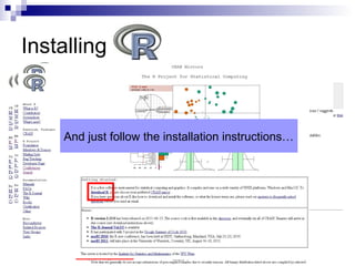
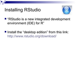
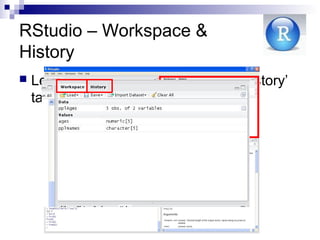
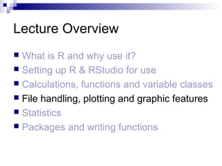
This document provides an overview of a lecture on R. The lecture will cover what R is and why to use it, setting up R and RStudio, performing calculations and functions in R, handling files and creating plots and graphics, performing statistical analyses, and writing functions. It also discusses R's strengths like data management, statistics, graphics, and its active user community, as well as weaknesses like not being very user friendly initially and being slower than other programming languages.

1. Introduction to
Dror Hollander
Gil Ast Lab
Sackler Medical School
29.4.12

2. Lecture Overview
 What is R and why use it?
 Setting up R & RStudio for use
 Calculations, functions and variable classes
 File handling, plotting and graphic features
 Statistics
 Packages and writing functions

3. What is ?
 “R is a freely available language and
environment for statistical computing and
graphics”
 Much like & , but bette !

4. Why use ?
 SPSS and Excel users are limited in their
ability to change their environment. The way
they approach a problem is constrained by
how Excel & SPSS were programmed to
approach it
 The users have to pay money to use the
software
 R users can rely on functions that have been
developed for them by statistical researchers
or create their own
 They don’t have to pay money to use them
 Once experienced enough they are almost
unlimited in their ability to change their
environment

5. ‘s Strengths
 Data management & manipulation
 Statistics
 Graphics
 Programming language
 Active user community
 Free

6.  Not very user friendly at start
 No commercial support
 Substantially slower than programming
languages (e.g. Perl, Java, C++)
‘s Weaknesses

7. Lecture Overview
 What is R and why use it?
 Setting up R & RStudio for use
 Calculations, functions and variable classes
 File handling, plotting and graphic features
 Statistics
 Packages and writing functions

8. Installing
 Go to R homepage:
http://www.r-project.org/
Choose a server
And just follow the installation instructions…

9. Installing RStudio
 “RStudio is a new integrated development
environment (IDE) for R”
 Install the “desktop edition” from this link:
http://www.rstudio.org/download/

10. Using RStudio
Script
editor
View help,
plots & files;
manage
packages
View variables in
workspace and
history file
R console

11.  Create your working directory
 Open a new R script file
Set Up Your Workspace

12. Lecture Overview
 What is R and why use it?
 Setting up R & RStudio for use
 Calculations, functions and variable classes
 File handling plotting and graphic features
 Statistics
 Packages and writing functions

13.  Operators take values (operands),
operate on them, and produce a new
value
 Basic calculations (numeric operators):
 + , - , / , * , ^
 Let’s try an example. Run this:
(17*0.35)^(1/3)
Before you do…
- Basic Calculations
Script editor
R console
Click here /
Ctrl+enter to
run code in
RStudio
Use “#” to write
comments
(script lines that
are ignored
when run)

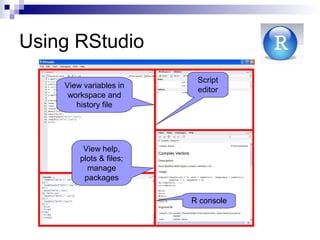
14.  All R operations are performed by functions
 Calling a function:
> function_name(x)
 For example:
> sqrt(9)
[1] 3
 Reading a function’s help file:
> ?sqrt
Also, when in doubt – Google it!
- Basic Functions
View help,
plots & files;
manage
packages

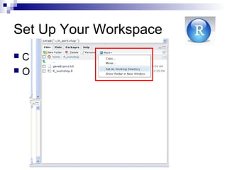
15.  A variable is a symbolic name given to
stored information
 Variables are assigned using either ”=” or
”<-”
> x<-12.6
> x
[1] 12.6
Variables

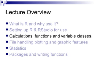
16.  A vector is a list of values. A numeric vector is composed of
numbers
 It may be created:
 Using the c() function (concatenate) :
x=c(3,7,9,11)
> x
[1] 3 7 9 11
 Using the rep(what,how_many_times) function (replicate):
x=rep(10,3)
 Using the “:” operator, signifiying a series of integers
x=4:15
Variables - Numeric Vectors

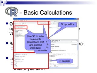
17.  Character strings are always double quoted
 Vectors made of character strings:
> x=c("I","want","to","go","home")
> x
[1] "I" "want" "to" "go" "home"
 Using rep():
> rep("bye",2)
[1] "bye" "bye"
 Notice the difference using paste() (1 element):
> paste("I","want","to","go","home")
[1] "I want to go home"
Variables - Character Vectors

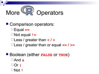
18.  Logical; either FALSE or TRUE
 > 5>3
[1] TRUE
 > x=1:5
> x
[1] 1 2 3 4 5
> x<3
[1] TRUE TRUE FALSE FALSE FALSE
Variables - Boolean Vectors

19. RStudio – Workspace &
History
 Let’s review the ‘workspace’ and ‘history’
tabs in RStudioView variables in
workspace and
history file

20.  Our vector: x=c(100,101,102,103)
 [] are used to access elements in x
 Extract 2nd
element in x
> x[2]
[1] 101
 Extract 3rd
and 4th
elements in x
> x[3:4] # or x[c(3,4)]
[1] 102 103
Manipulation of Vectors

21.  > x
[1] 100 101 102 103
 Add 1 to all elements in x:
> x+1
[1] 101 102 103 104
 Multiply all elements in x by 2:
> x*2
[1] 200 202 204 206
Manipulation of Vectors –
Cont.

22. More Operators
 Comparison operators:
Equal ==
Not equal !=
Less / greater than < / >
Less / greater than or equal <= / >=
 Boolean (either FALSE or TRUE)
And &
Or |
Not !

23.  Our vector: x=100:150
 Elements of x higher than 145
> x[x>145]
[1] 146 147 148 149 150
 Elements of x higher than 135 and lower than
140
> x[ x>135 & x<140 ]
[1] 136 137 138 139
Manipulation of Vectors –
Cont.

24.  Our vector:
> x=c("I","want","to","go","home")
 Elements of x that do not equal “want”:
> x[x != "want"]
[1] "I" "to" "go" "home"
 Elements of x that equal “want” and “home”:
> x[x %in% c("want","home")]
[1] "want" "home"
Manipulation of Vectors –
Cont.
Note: use “==” for 1 element and “%in%” for several elements

25.  A data frame is simply a table
 Each column may be of a different class
(e.g. numeric, character, etc.)
 The number of elements in each
row must be identical
Variables – Data Frames
age gender disease
50 M TRUE
43 M FALSE
25 F TRUE
18 M TRUE
72 F FALSE
65 M FALSE
45 F TRUE
 Accessing elements in
data frame:
x[row,column]
The ‘age’ column:
> x$age # or:
> x[,”age”] # or:
> x[,1]
All male rows:
> x[x$gender==“M”,]

26.  A matrix is a table of a different class
 Each column must be of the same class
(e.g. numeric, character, etc.)
 The number of elements in each
row must be identical
Variables – Matrices
 Accessing elements in
matrices:
x[row,column]
The ‘Height’ column:
> x[,”Height”] # or:
> x[,2]
Note: you cannot use “$”
> x$Weight

27. Exe cise
 Construct the character vector ‘pplNames’
containing 5 names: “Srulik”, “Esti”, ”Shimshon”,
“Shifra”, “Ezra”
 Construct the numeric vector ‘ages’ that includes
the following numbers: 21, 12 (twice), 35 (twice)
 Use the data.frame() function to construct
the ‘pplAges’ table out of ‘pplNames’ & ‘ages’
 Retrieve the ‘pplAges’ rows with ‘ages’ values
greater than 19

28. Lecture Overview
 What is R and why use it?
 Setting up R & RStudio for use
 Calculations, functions and variable classes
 File handling, plotting and graphic features
 Statistics
 Packages and writing functions

29.  For example: analysis of a gene expression file
 Workflow:
 Save file in workspace directory
 Read / load file to R
 Analyze the gene expression table
 305 gene expression reads in 48 tissues (log10 values
compared to a mixed tissue pool)
 Values >0  over-expressed genes
 Values <0  under-expressed genes
 File includes 306 rows X 49 columns
Wo king With a File

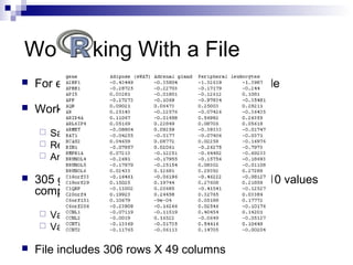
30.  Read file to R
 Use the read.table() function
 Note: each function receives input (‘arguments’) and produces
output (‘return value’)
 The function returns a data frame
 Run:
> geneExprss = read.table(file =
"geneExprss.txt", sep = "t",header = T)
 Check table:
> dim(geneExprss) # table dimentions
> geneExprss[1,] # 1st line
File Handling - ead File

31. Plotting - Pie Chart
 What fraction of lung genes
are over-expressed?
 What about the under-
expressed genes?
 A pie chart can illustrate our
findings
1
2
3
4
5
6
7
8 9
10

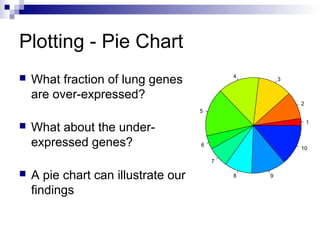
32. Using the pie() Function
 Let’s regard values > 0.2 as over-
expressed
 Let’s regard values < (-0.2) as under-
expressed
 Let’s use Length()  retrieves the
number of elements in a vector
> up = length (geneExprss$Lung
[geneExprss$Lung>0.2])
> down = length (geneExprss$Lung
[geneExprss$Lung<(-0.2)])
> mid = length (geneExprss$Lung
[geneExprss$Lung<=0.2 &
geneExprss$Lung>=(-0.2)])
> pie (c(up,down,mid) ,labels =
c("up","down","mid"))

33. Plotting - Scatter Plot
 How similar is the gene
expression profile of the
Hippocampus (brain) to
that of that of the Thalamus
(brain)?
 A scatter plot is ideal for
the visualization of the
correlation between two
variables

34. Using the plot() Function
 Plot the gene expression profile of
Hippocampus.brain against that of
Thalamus.brain
 > plot
( geneExprss$Hippocampus.brain,
geneExprss$Thalamus.brain,
xlab="Hippocampus", ylab="Thalamus")

35.  .RData files contain saved R environment data
 Load .RData file to R
 Use the load() function
 Note: each function receives input (‘arguments’) and produces
output (‘return value’)
 Run:
> load (file = "geneExprss.RData")
 Check table:
> dim(geneExprss) # table dimentions
> geneExprss[1,] # 1st line
> class(geneExprss) # check variable class
File Handling – Load File to

36. Plotting – Bar Plot
 How does the
expression profile of
“NOVA1” differ across
several tissues?
 A bar plot can be used
to compare two or more
categories

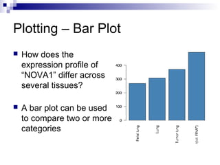
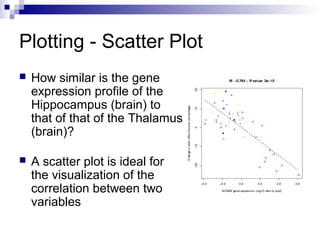
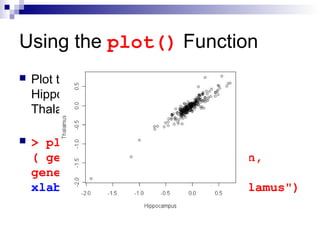
37. Using the barplot() Function
 Compare “NOVA1” expression in Spinalcord, Kidney,
Heart and Skeletal.muscle by plotting a bar plot
 Sort the data before plotting using the sort() function
 barplot() works on a variable of a matrix class
 > tissues = c ( "Spinalcord", "Kidney",
"Skeletal.muscle", "Heart")
> barplot ( sort ( geneExprss
["NOVA1",tissues] ) )

38. More Graphic Functions to Keep in
Mind
 hist()
 boxplot()
 plotmeans()
 scatterplot()

39. Exe cise
 Use barplot() to compare “PTBP1” &
“PTBP2” gene expression in
“Hypothalamus.brain”
 Use barplot() to compare “PTBP1” &
“PTBP2” gene expression in “Lung”
 What are the differences between the two plots
indicative of?

40. Save Plot to File - RStudio
 Create a .PNG file
 Create a .PDF file

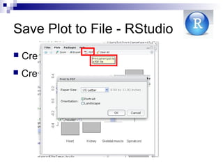
41.  Before running the visualizing function, redirect
all plots to a file of a certain type
jpeg(filename)
png(filename)
pdf(filename)
postscript(filename)
 After running the visualization function, close
graphic device using dev.off() or
graphcis.off()
Save Plot to File in
 For example:
> load(file="geneExprss.RData")
> Tissues = c ("Spinalcord", "Kidney",
"Skeletal.muscle", "Heart")
> pdf("Nova1BarPlot.PDF")
> Barplot ( sort (geneExprss ["NOVA1",
tissues] ) )
> graphics.off()

42. Lecture Overview
 What is R and why use it?
 Setting up R & RStudio for use
 Calculations, functions and variable classes
 File handling, plotting and graphic features
 Statistics
 Packages and writing functions

43. Statistics – cor.test()
 A few slides back we compared the expression
profiles of the Hippocampus.brain and the
Thalamus.brain
 But is that correlation statistically significant?
 R can help with this sort of question as well
 To answer that specific question we’ll use the
cor.test() function
> geneExprss = read.table (file =
"geneExprss.txt", sep = "t", header = T)
> cor.test ( geneExprss$Hippocampus.brain,
geneExprss$Thalamus.brain, method =
"pearson")
> cor.test ( geneExprss$Hippocampus.brain,
geneExprss$Thalamus.brain, method =
"spearman")

44.  t.test() # Student t test
 wilcox.test() # Mann-Whitney test
 kruskal.test() # Kruskal-Wallis rank sum test
 chisq.test() # chi squared test
 cor.test() # pearson / spearman correlations
 lm(), glm() # linear and generalized linear models
 p.adjust() # adjustment of P-values for multiple
testing (multiple testing correction) using FDR,
bonferroni, etc.
Statistics – More Testing, FYI

45.  Use the summary() function
 > geneExprss = read.table (file =
"geneExprss.txt", sep = "t", header = T)
 > summary(geneExprss$Liver)
 Min. -1.84400
1st Qu. -0.17290
Median -0.05145
Mean -0.08091
3rd Qu. 0.05299
Max. 0.63950
Statistics – Examine the
Distribution of Your Data

46.  mean()
 median()
 var()
 min()
 max()
 When using most of these functions remember to use
argument na.rm = T
Statistics – More Distribution
Functions

47. Lecture Overview
 What is R and why use it?
 Setting up R & RStudio for use
 Calculations, functions and variable classes
 File handling, plotting and graphic features
 Statistics
 Packages and writing functions

48.  All operations are performed by functions
 All R functions are stored in packages
 Base packages are installed along with R
 Packages including additional functions can by
downloaded by user
 Functions can also be written by user
Functions & Packages

49. Install & Load Packages -
RStudio
Check to load
package

50. Install & Load Packages -
 Use the functions:
Install.packages(package_name)
update.packages(package_name)
library(package_name) # Load a
package

51.  Reading the functions’ help file
(> ?function_name)
 Run the help file examples
 Use http://www.rseek.org/
 Google what you’re looking for
 Post on the R forum webpage
 And most importantly – play with it, get the hang of it,
and do NOT despair 
Final Tips
R