The document discusses analyzing a movie dataset to understand predictors of audience score. It loads necessary packages and the movie data. Exploratory data analysis is performed, including checking data structure, selecting relevant variables for modeling, removing missing data, summarizing variables, and graphically analyzing relationships. Runtime is found to have a weak positive linear relationship with audience score based on a scatterplot, while release year and month show no clear relationships. Correlation analysis will further examine relationships between predictors and the response variable, audience score.

1. ---
title: "Assignment: Modeling and prediction for movies"
output:
html_document:
fig_height: 4
highlight: pygments
theme: spacelab
---
## Setup
### Load packages
```{r load-packages, message = FALSE}
library(ggplot2)
library(dplyr)
library(statsr)
library(corrplot)
library(leaps)
library(grid)
library(gridExtra)
```
### Load data
Make sure your data and R Markdown files are in the same directory. When loaded
your data file will be called `movies`. Delete this note when before you submit
your work.
```{r load-data}
setwd("E:/R WD")
load("E:/R WD/movies.RData")
```
* * *
## Part 1: Data
Dataset was downloaded from Coursera assigment webpage which comes from IMDB and Rotten Tomatoes.The observation
consists of random samples complied from the reviews of the audience and critics.The dataset contains information
about 651 movies released before 2016 and information about these are stored across 32 variables. The data is randomly
selected not randomly assigned. Consequently any conclusion can only be generlised to population; causality requires
random assignment. Hence with this dataset it is only possible to do a n observationa study & no causal analysis cn be
done.
* * *
## Part 2: Research question
After having a look at the data I concluded that I will try to understanding the most significant predictor and its
relationship with audience score for a movie i.e movies polularity.
* * *
## Part 3: Exploratory data analysis
### Analyse the Data
Checking the structure of the data using the code below.
```{r}
str(movies)
```
##### Discussion
On analysing the structure of movie dataset, we can conclude that the dataset cantains 32 variables and 651
observations. Among the total 32 variables, 9 ar character variables, 12 are factor variable, 10 are numerical
variable, one is integer variable and among the present 10 numerical variable 6 are related to date. There are a total
of four variables related to rating and these are Mpaa_rating, Imdb_rating, critics_rating, and audience_ rating. Two
of these variable is related to scoring a movie, one variable related to the maturity content of the movie and one to
the voting for a movie.
For identification of the popularity of the movies not all variable will be relevant. Also for variable like awards
are not taken into consideration here as awards ceremony happens much after the movie is released and won't be
affecting the audience score. the variables like actor1,2,3,4,5, URL based, and studio won't not taken into
consderation.
### Getting Data for the model
Getting the data of the potential predictor for the model using the code below.
```{r}
# Selected data will be saved to variabe named MD signifying model data
# Here Pipe operator %>% is used which basically tells R to take the value of that which is to the left and pass it to
the right as an argument.
MD <- movies %>%
# from the movie dataset selecting these
select (title_type, genre, runtime,

2. mpaa_rating, thtr_rel_year, thtr_rel_month,
imdb_rating, imdb_num_votes, critics_score,
critics_rating, audience_rating, audience_score)%>%
# out of the selected renaming some long variables name
rename (rel_month = thtr_rel_month, rel_year = thtr_rel_year)
```
### Analyze the structure of Model Data
Checking the structure of the selected data from the movie data using the code below.
```{r}
str(MD)
```
##### Discussion
On analysing the structure of Model Data dataset, we can conclude that the dataset cantains 12 variables out of the
initial 32 variables and 651 observations. Among the total 12 variables, 5 are factor variable, 6 are numerical
variable, one is integer variable and among the present 6 numerical variable 2 are related to date. There are a total
of four variables related to rating and these are Mpaa_rating, Imdb_rating, critics_rating, and audience_ rating. Two
of these variable is related to scoring a movie, one variable related to the maturity content of the movie and one to
the voting for a movie.
### Removing missing data and Check dimentionality
Removing the obseravtion having missing data in the Model Data dataset using the code below.
```{r}
# Remove NAs
CompleteCases_Index <-complete.cases(MD)
MD <- MD[CompleteCases_Index, ]
dim(MD)
```
##### Discussion
Initially there 651 obseravations present and now after removing the incomplete obseravtions we are left with 650
observations i.e. we had a 651-650=1 incomplete observations
### Summarize of Model Data
```{r}
summary(MD)
```
##### Discussion
Out of the total 650 complete observations of the movies, 591 are feature films, 54 are documentry and 5 are TV
Movies.
Among these movies 305 are drama based, 87 are comedy based, 65 are action & adventure based, 59 are mystery &
suspense based, 51 are documentry, 23 are horror and the 60 lies in other categories.
Run time of movies ranges from 39 minutes to 267 minutes and it seems to be right skewed.
Among these movies 19 are G rated, 2 are NC-17 rated, 118 are PG rated, 133 are PG-13 rated, 329 are R rated and 49
are Unrated.
Movies release year for the available data ranges from 1970 to 2014 and the the data is a bit left skewed.
Movies release month shows that more number of movies are released in the later half of the year.
The rating score for the IMDB rating ranges from 0 to 9 while critics score and audience score ranges from 1 to 100.
IMDB rating, critics score and audience score all are skewed left. IMDB num votes ranges from 180 to 893008 and this
is right skewed.
The critics rating has three level of which for majority are negative (i.e. 307). In contrast audience rating has two
levels of which majority are positive (i.e. 375).
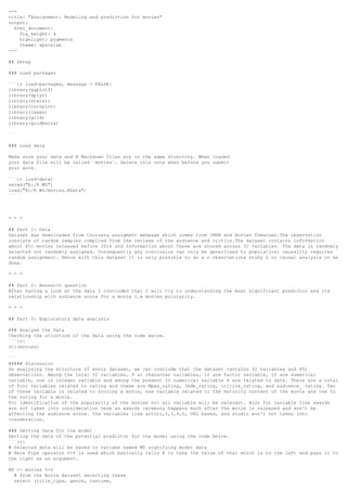
#### Analyze the above discussion graphically
Checking the skewedness of various parameters using histogram and plot using the code below.
```{r}
# giving a layout so that the output of all the function below don't show up individually but together
#layout(matrix(c(1,2,3,4), nrow=3, ncol=1, byrow= TRUE))
#par(mfrow = c(2,1))
plot(MD$title_type, xlab = "Movies Type", ylab = "no. of movies", las = 0, main="a) No. of movies of specific type",
col=rainbow(7))
plot(MD$genre, xlab = "Movies Genre", ylab = "no. of movies", las = 2, axis=0.6, main="b) No. of movies of specific
genre", col=rainbow(7), col.lab = "Black", col.axis="dark grey")
hist(MD$runtime, xlab = "Movie Runtime", prob=TRUE, main = "c) Runtime Evaluation")
lines(density(MD$runtime), col="blue", lwd=2)
plot(MD$mpaa_rating, xlab = "mpaa rating", ylab = "no. of movies", las = 0, main="d) Classification of no. of movies
based on mpaa rating", col=rainbow(7), cex.lab = 1, col.lab = "Black")
hist(MD$rel_year, xlab = "Movie release year", xlim = c(1970, 2014), breaks = 44, prob=TRUE, main = "e) No. of movies
released per year distribution")
lines(density(MD$rel_year), col="blue", lwd=2)
hist(MD$rel_month, xlim = c(1, 12), breaks = 12, xlab = "Movie release month", prob=TRUE, main = "f) Movie Release
Month distribution")
lines(density(MD$rel_month), col="blue", lwd=2)
hist(MD$imdb_rating, xlab = "imdb rating", breaks = 18, prob=TRUE, main = "g) Movie IMDB rating")
lines(density(MD$imdb_rating), col="blue", lwd=2)
hist(MD$imdb_num_votes, xlim = c(180, 893008), breaks = 500, xlab = "imdb no. of votes", prob=TRUE, main = "h) Movie
imdb number of votes")

3. lines(density(MD$imdb_num_votes), col="blue", lwd=2)
hist(MD$critics_score, xlab = "Critics score", xlim = c(1, 100), breaks = 20, prob=TRUE, main = "i) Critics score of
the movie")
lines(density(MD$critics_score), col="blue", lwd=2)
plot(MD$critics_rating, xlab = "Critics Rating", ylab = "no. of movies", las = 0, main="j) No. of movies classified
by critics rating", col=rainbow(7))
plot(MD$audience_rating, xlab = "Audience Rating", ylab = "no. of movies", las = 0, main="k) No. of movies classified
by audience Rating", col=rainbow(7))
hist(MD$audience_score,xlim = c(1, 100), breaks = 20, xlab = "Audience Score", prob=TRUE, main = "k) Movie Audience
Score")
lines(density(MD$audience_score), col="blue", lwd=2)
```
##### Discussion
The discussion done above seems to be adequate even on observing the graphical interpretation.
#### **Understandanding the relationship between various numerical parameter and audience score**
#### Graph the runtime predictor
Checking the relationship between runtime (explanatory variable) and audience score (response variable) by plotting
using the code below.
```{r}
ggplot(MD, aes(x=runtime, y=audience_score)) + geom_point() + stat_smooth(method=lm, level=0.99)
```
##### Discussion
The relationship is a positive weak liner relationship between a potential explanatory variable (predictor) and the
response variable as depicted in the graph. This Relationship should be confirmed by the Corelation matrix (done
below).
#### Graph the rel_year predictor
Checking the relationship between rel_year (explanatory variable) and audience score (response variable) by plotting
using the code below.
```{r}
ggplot(MD, aes(x=rel_year, y=audience_score)) + geom_point() + stat_smooth(method=lm, level=0.99)
```
##### Discussion
There seems to be no relationship between a potential explanatory variable (predictor) and the response variable as
depicted in the graph. This Relationship should be confirmed by the Corelation matrix (done below).
#### Graph the rel_month predictor
Checking the relationship between rel_month (explanatory variable) and audience score (response variable) by plotting
using the code below.
```{r}
ggplot(MD, aes(x=rel_month, y=audience_score)) + geom_point() + stat_smooth(method=lm, level=0.99)
```
##### Discussion
There seems to be no relationship between a potential explanatory variable (predictor) and the response variable as
depicted in the graph. This Relationship should be confirmed by the Corelation matrix (done below).
#### Graph the imdb_rating predictor
Checking the relationship between imdb_rating (explanatory variable) and audience score (response variable) by
plotting using the code below.
```{r}
ggplot(MD, aes(x=imdb_rating, y=audience_score)) + geom_point() + stat_smooth(method=lm, level=0.99)
```
##### Discussion
There seems to be strong positive linear relationship between a potential explanatory variable (predictor) and the
response variable as depicted in the graph. This Relationship should be confirmed by the Corelation matrix (done
below).
#### Graph the imdb_num_votes predictor
Checking the relationship between imdb_num_votes (explanatory variable) and audience score (response variable) by
plotting using the code below.
```{r}
ggplot(MD, aes(x=imdb_num_votes, y=audience_score)) + geom_point() + stat_smooth(method=lm, level=0.99)
```
##### Discussion
There seems to be a moderate positive linear relationship between a potential explanatory variable (predictor) and the
response variable as depicted in the graph. This Relationship should be confirmed by the Corelation matrix (done
below).
#### Graph the critics_score predictor
Checking the relationship between imdb_num_votes (explanatory variable) and audience score (response variable) by
plotting using the code below.
```{r}
ggplot(MD, aes(x=critics_score, y=audience_score)) + geom_point() + stat_smooth(method=lm, level=0.99)
```

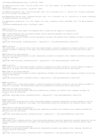
4. ##### Discussion
There seems to be a strong positive linear relationship between a potential explanatory variable (predictor) and the
response variable as depicted in the graph. This Relationship should be confirmed by the Corelation matrix (done
below).
#### **Creating a Corelation Matrix and Graphing it**
Corelation matrix was created using the code below.
```{r}
# Selecting the numerical data
MD[ , sapply(MD, is.numeric)]
# applying the numerical data to get correlation
CorMatrix <- cor(MD[ ,sapply(MD,is.numeric)], use= "complete.obs")
corrplot(CorMatrix, method="shade", shade.col=NA, cl.pos="n", tl.col="black", tl.srt=30, addCoef.col="black")
```
##### Discussion
The correlation matrix gives the following corelationship coefficient between the numeric predictor and reponse
variable which is audience_score is as below.
|SNo.| Predictor |Correlation Coeff.| Linear Relationship |
|----|---------------|------------------|------------------------|
| 1. | runtime | 0.18 |+ve, weak relationship |
| 2. | rel_year | -0.05 |no relationship |
| 3. | rel_month | 0.03 |no relationship |
| 4. | imdb_rating | 0.86 |+ve, very strong |
| 5. | imdb_num_votes| 0.29 |+ve, moderate |
| 6. | critics_score | 0.70 |+ve, strong |
:
In the correlation matrix it can be seen that the collinearty between two explanatory variable imdb_rating and
critics_score. the relationship between these two is exceptionally strong which is 76% and it means that the two
variables contribute redundant information to the model and complicate model estimation. Hence the explanatory
variable, **critics_score will not be used**. However the extremely high correlation between imdb_rating and
audience_score of 86% indicates that imdb_rating should be the first predictor added to the model.
* * *
## Part 4: Modeling
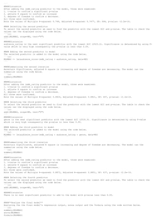
####**Developing the Model**
To create a Multiple Linear Regression (MLR) model that predicts audience score (AS), adding predictor with Forwad
Stepwise Regression methodology has been selected.
To build/create the multiple regression model a iterative process is used. the model will be build using the lm()
function, Summarizing the model and to analyze its adjusted R square the summary function is used. To add the
predictor to the model by analyzing both the AIC & p-value, add() function is used.
This approach was used because it evaluated both the significance (as measured by both F-values and t-values) and the
proportion of variability (as measured by adjusted R-square) before a predictor is added.
#### Create blank Model for audience score
Create a blank model for audience score (response variable) using the code below.
```{r}
# Multiple Linear Regression Model for Audience Score
MLRMAS <- lm(audience_score~1, data=MD)
```
#### Summarze the existing model
ascertain significane, adjusted R-square, is increasing & the degree of freedom are decreasing
```{r}
summary(MLRMAS)
```
#####Discussion
Only the intercept is in the model and there is no predictor. However the degree of freedom is 649 (650-0-1).
#### Selecting the first predictor
To select the first predictor we need to find the predictor with the lowest AIC and p-value. The table to check the
values can the displayed using the code below.
```{r}
add1(MLRMAS, scope=MD, test="F")
```
#####Discussion
As expected, the significant predictor with the lowest AIC is imdb_rating (3016.5). significance is determined by
using F-value which is very high consequently the p-value is less than 0.05.
#### Adding the first predictor to model
The selected predictor is added to the model using the code below.
```{r}
MLRMAS <- lm(audience_score~imdb_rating, data=MD)
```
####Summarizing the first iteration
Ascertain Significance, adjusted R square is increasing and degree of freedom are decreasing. The model can the
summarize using the code below.
```{r}
summary(MLRMAS)

5. ```
####Discussion
After adding the imdb_rating predictor to the model, three were examined:
1. t-value to confirm a significant p-value
2. adjuste R square to confirm an increase
3. degrees of freedom to confirm a decrease.
All three were confirmed.
Note the values of Multiple R-squared: 0.748, Adjusted R-squared: 0.7477, DF: 648, p-value: <2.2e-16.
#### Selecting the second predictor
To select the second predictor we need to find the predictor with the lowest AIC and p-value. The table to check the
values can the displayed using the code below.
```{r}
add1(MLRMAS, scope=MD, test="F")
```
#####Discussion
audience_rating is the next significant predictor with the lowest AIC (2523.2). Significance is determined by using F-
value which is very high consequently the p-value is less than 0.05.
#### Adding the second predictor to model
The selected predictor is added to the model using the code below.
```{r}
MLRMAS <- lm(audience_score~imdb_rating + audience_rating, data=MD)
```
####Summarizing the second iteration
Ascertain Significance, adjusted R square is increasing and degree of freedom are decreasing. The model can the
summarize using the code below.
```{r}
summary(MLRMAS)
```
####Discussion
After adding the imdb_rating predictor to the model, three were examined:
1. t-value to confirm a significant p-value
2. adjuste R square to confirm an increase
3. degrees of freedom to confirm a decrease.
All three were confirmed.
Note the values of Multiple R-squared: 0.8824, Adjusted R-squared: 0.8821, DF: 647, p-value: <2.2e-16.
#### Selecting the third predictor
To select the second predictor we need to find the predictor with the lowest AIC and p-value. The table to check the
values can the displayed using the code below.
```{r}
add1(MLRMAS, scope=MD, test="F")
```
#####Discussion
genre is the next significant predictor with the lowest AIC (2516.3). Significance is determined by using F-value
which is very high consequently the p-value is less than 0.05.
#### Adding the third predictor to model
The selected predictor is added to the model using the code below.
```{r}
MLRMAS <- lm(audience_score~imdb_rating + audience_rating + genre, data=MD)
```
####Summarizing the third iteration
Ascertain Significance, adjusted R square is increasing and degree of freedom are decreasing. The model can the
summarize using the code below.
```{r}
summary(MLRMAS)
```
####Discussion
After adding the imdb_rating predictor to the model, three were examined:
1. t-value to confirm a significant p-value
2. adjuste R square to confirm an increase
3. degrees of freedom to confirm a decrease.
All three were confirmed.
Note the values of Multiple R-squared: 0.8872, Adjusted R-squared: 0.8851, DF: 637, p-value: <2.2e-16.
#### Selecting the fourth predictor
To select the second predictor we need to find the predictor with the lowest AIC and p-value. The table to check the
values can the displayed using the code below.
```{r}
add1(MLRMAS, scope=MD, test="F")
```
#####Discussion
There is no next significant predictor to add to the model with p-value less than 0.05.
####**Analyze the final model**
Analyzing the the final model's regression output, avona output and the formula using the code written below.
```{r}
summary(MLRMAS)
anova(MLRMAS)
formula(MLRMAS)

6. ```
##### Discussion
The final model depicts a Parsimonius Model: the simplest model with the highest predictive power. Only three
predictors are used : imdb_rating, audience_rating and genre.
The ANOVA output confirms the significance of the individual predictors (i.e., p-values < 0.05)
The linear regression model output confirm the significance of the individual predictors as well, but it also confirms
the significance of the model as a whole (i.e., F-statistic 417.5 on 12 and 637 DF, p-value:< 2.2e-16).
Finally, the proportion of variability in the response variable explained by the model is 88.51% (i.e. adjusted R-
square).
Variables that were excluded from the table are listed below-
runtime - weak linear relationship and not significant
rel_year - no linear relationship and not significant
rel_month - no linear relationship and not significant
mpaa_rating - not significant
imdb_num_votes - not significant
critics_rating - not significant
critics_score - collinearity and not significant
#### Intrepreting the coefficients
To know of the coefficient of the model use the code below.
```{r}
coefficients(MLRMAS)
```
#####Discussion
the interpretation of a multivariate regression coefficient is the expected change in the response per unit change in
a predictor, holding all of the other predictors constant.
Specific interpretations follow-
* Intercept Coefficient:
the estimated audience score is -12.56053 if none of the predictors in the model are included. this cn be interpreted
as that if no information is given the audience generally conceive the movie with a negative sense.
* imdb_rating:
the estimated expected increase in the audience score is 9.8028 when the imdb_rating goes up by 1, holding all other
predictors constant.
* audience_rating Upright coefficient:
the estimted audience_rating score is 20.318, ehen the audience rating is "Upright " and holding all other predictors
constant. However if the audience rating is "Spilled" the expected decrease in audience score will be of around 20.
* genreDrama Coefficient:
the estimated decrease in audience score, when the genre is drama is 0.83394, while holding all other predictor
constant. However, the audience scores can increase or decrease depending on what genre category is selected.
####**Model Diagnostics i.e. Checking the conditions graphically**
####Check for linearity
Checking for the linear relationship between numerical predictor (s) and residual (s) using the code written below.
```{r}
plot(MLRMAS$residuals ~ MD$imdb_rating, main="Linearity Condition")
```
#####Discussion
Condition met the plot depicts a complete random scatter around zero; no descernable pattern.
####Check for normality
Checking for the nearly normal residuals using the code written below.
```{r}
qqnorm(MLRMAS$residuals, main="Normality Condition")
qqline(MLRMAS$residuals, main="Normality Condition")
```
#####Discussion
Condition met - the majority of the points lie on the line, but because of skeness, a few points do not. Also note
that there are no apparent outliners.
```{r}
hist(MLRMAS$residuals, prob=TRUE, main="Normality Condition")
lines(density(MLRMAS$residuals), col="blue", lwd=2)
```
#####Discussion
Condition met - the histogram confirms the skewness (right skewness) but the distribution still appear to be nearly
normal.
####Check for variability
checking for the variability of the residuals using the code written below.
```{r}
plot(MLRMAS$residuals ~ MLRMAS$fitted.values, main="Variability conditions")
```
#####Discussion
Condition met - the plot of predicted values shows that residuals are equally variable for low and heigh values and
there is no visible fan pattern.

7. ```{r}
plot(abs(MLRMAS$residuals) ~ MLRMAS$fitted.values, main="Variability conditions")
```
#####Discussion
Condition met - the plot of absolute value of the residuals does not depict any unusual observations.
####Check for independancy
checking for the independancy of the residuals using the code written below.
```{r}
plot(MLRMAS$residuals, main="Independany Conditions")
```
#####Discussion
Condition met - the plot depicts residuals being randomly scatterd around zero.
* * *
## Part 5: Prediction
####**Building a test data case**
Build test data cases for the movie "Deadpool (2016)" using the data gathered from IMDB and rotten tomatoes website
and storing the data in the variable named TDC (test data case) using the following code.
```{r}
audience_score <- 90
imdb_rating <- 8.1
audience_rating <- "Upright"
genre <- "Comedy"
TDC <- data.frame (audience_score, imdb_rating, audience_rating, genre)
```
#####Discussion:
as said above the source of the data is IMDB and rotten tomatatoes website. once the movie was selected the movie ws
searched on these two website and the reuired data was extracted which will be used here.
####Predicting the audience score
TDC (test data case) using the following code.
```{r}
myPrediction <- round(predict(MLRMAS, TDC), digits = 0)
c(myPrediction, TDC$audience_score)
```
#####Discussion:
Predicting the correct audience score was not easy. The model seems to be much sensitive to the imdb_rating variable
and the result of this sesitivity was to predict a much higher audience score.
Audience score will be predicted much more accurately by the model when both the audience acore and the imdb_rating
are relatively high.
####Estimate and Interpret the prediction confidence interval
```{r}
ConfidenceInterval <- predict(MLRMAS, TDC, interval="confidence")
ConfidenceInterval
```
#####Discussion:
We are 95% confident that, all else being equal, the predicted audience score for the movie 'Deadpool' will be between
86.72074 and 90.62207 on average.
* * *
## Part 6: Conclusion
Explanatory data analysis was of great help in providing the insight on what data items to include in the model or not
to.
The modeling methodology of evaluating both significance and variablity of each predictor before adding it to the
model produced a very robust model that very precisely answered the research question and the model predicted the
audience score correctly and the margin of error is +/- (90.62207-86.72074) =1.950665.
#####State Concerns
Sample is not representative: the data is biased toward drama movies, consequently the model was trained primarily by
drame movie dataset thus it would have been better to predict the audience score about drama movies.