This documentation describes the process of creating a recommendation system using Neo4j. The Data Mining techniques used are the Apriori algorithm on Hana, the PCA and the KMeans on SPSS. The dataset used is the MovieLens Dataset

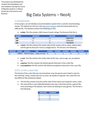
1. Big Data Systems – Neo4j
1.Introduction
In this project, we will develop a recommendation system that is used for recommending
movies. The dataset we will use is the MovieLens Dataset and more particularly the ml-
100k.zip file. This dataset contains the following csv files:
 u.data: This file contains 100 k rows of movie ratings. The format of the file is:
USERID MOVIEID RATING TIMESTAMP
100 23 4 88897654
100 3 2 87665445
101 3 3 79978699
 u.item: This file contains the master data of the movies such as name, release date,
and the genres that each movie is categorized as. The format is the following
MOVEID NAME RelDate URL GENRE1 GENRE2 GENRE3 GENRE4 GENRE5 ….
1 FARGO Dd/mm/yyyy www.url.com 0 1 1 0 0 0
 u.user: This file contains the master data of the user, such as age, sex, occupation
etc.
 u.genres: this file contains the distinct genres that exist in the u.item file
 u.occupations: this file contains the distinct occupations that exist in the u.user file
2.ETL in the u.item file
The format of the u.item file was not normalized, since the genres were listed in columns
like a bitmap. Using a simple tool such as excel, we decide to separate the u.item file into
two different files (relational tables).
 The first file contains only the master data of the movie and it kept the name u.item
 The second file is a join table/file between the new u.item file and the u.genres file,
since according to the dataset, each movie can belong to many genres. The format is
the following:
MOVIEID GENREID
1 1
1 2
2 5
This project was developed by
students Ilias Katsabalos and
Leon Kalderon during the course
of Big Data Systems in Athens
University of Economics and
Business

2. 3.Data model in Neo4j
Above you can see the model of the data in Neo4j. As you can see we have the following
nodes and vertices:
 Nodes:
o Users: Holds the information of each user
o Occupation: The master data of the occupation
o Movie: The master data of the movie
o Genre: The master data of the genres
 Relationships:
o Rated: connects the users with the movies, and has the rating as a property
in the relationship
o Works: Connects the users with their occupations
o Characterized: Connects the movies with their genres
4.Data mining on the given dataset
So far we have just utilized the data included in the ml-100k dataset. Now, in order to
implement our recommendation system, we need to mine some additional information on
the given dataset.
4.1 Mining association rules
By mining association rules between the movies, we can create a new relationship amongst
them that connects the pre rule with its post rule. The u.data file may serve the purpose of a
transaction table that we can implement the apriori algorithm on. The platform that we
decided to use is the HANA Cloud Platform. We inserted the u.data file and execute the
algorithm. The code for the execution of the algorithm is the following:
SET SCHEMA "SYSTEM";
DROP TYPE PAL_APRIORI_DATA_T;
CREATE TYPE PAL_APRIORI_DATA_T AS TABLE(
ID:
Name:
Age:
ID:
Name:
URL:
ID:
Name:
ID:
Name:
User Occupation
Movie Genre
Characterized
RATED
Rate:
Works

3. "TRANSID" VARCHAR(100),
"ITEM" VARCHAR(100)
);
DROP TYPE PAL_APRIORI_RESULT_T;
CREATE TYPE PAL_APRIORI_RESULT_T AS TABLE(
"PRERULE" VARCHAR(500),
"POSTRULE" VARCHAR(500),
"SUPPORT" DOUBLE,
"CONFIDENCE" DOUBLE,
"LIFT" DOUBLE
);
DROP TYPE PAL_APRIORI_PMMLMODEL_T;
CREATE TYPE PAL_APRIORI_PMMLMODEL_T AS TABLE(
"ID" INTEGER,
"PMMLMODEL" VARCHAR(5000)
);
DROP TYPE PAL_CONTROL_T;
CREATE TYPE PAL_CONTROL_T AS TABLE(
"NAME" VARCHAR(100),
"INTARGS" INTEGER,
"DOUBLEARGS" DOUBLE,
"STRINGARGS" VARCHAR (100)
);
DROP TABLE PAL_APRIORI_PDATA_TBL;
CREATE COLUMN TABLE PAL_APRIORI_PDATA_TBL(
"POSITION" INT,
"SCHEMA_NAME" NVARCHAR(256),
"TYPE_NAME" NVARCHAR(256),
"PARAMETER_TYPE" VARCHAR(7)
);
INSERT INTO PAL_APRIORI_PDATA_TBL VALUES (1, 'SYSTEM',
'PAL_APRIORI_DATA_T', 'IN');
INSERT INTO PAL_APRIORI_PDATA_TBL VALUES (2, 'SYSTEM', 'PAL_CONTROL_T',
'IN');
INSERT INTO PAL_APRIORI_PDATA_TBL VALUES (3, 'SYSTEM',
'PAL_APRIORI_RESULT_T', 'OUT');
INSERT INTO PAL_APRIORI_PDATA_TBL VALUES (4, 'SYSTEM',
'PAL_APRIORI_PMMLMODEL_T', 'OUT');
CALL "SYS".AFLLANG_WRAPPER_PROCEDURE_DROP('SYSTEM',
'PAL_APRIORI_RULE_PROC');
CALL "SYS".AFLLANG_WRAPPER_PROCEDURE_CREATE('AFLPAL', 'APRIORIRULE',
'SYSTEM', 'PAL_APRIORI_RULE_PROC', PAL_APRIORI_PDATA_TBL);
DROP TABLE PAL_APRIORI_TRANS_TBL;
CREATE COLUMN TABLE PAL_APRIORI_TRANS_TBL LIKE PAL_APRIORI_DATA_T;
INSERT INTO PAL_APRIORI_TRANS_TBL (SELECT USERID, MOVIEID FROM
"SYSTEM"."RATINGS");
DROP TABLE #PAL_CONTROL_TBL;
CREATE LOCAL TEMPORARY COLUMN TABLE #PAL_CONTROL_TBL(
"NAME" VARCHAR(100),
"INTARGS" INTEGER,

4. "DOUBLEARGS" DOUBLE,
"STRINGARGS" VARCHAR (100)
);
INSERT INTO #PAL_CONTROL_TBL VALUES ('THREAD_NUMBER', 2, null, null);
INSERT INTO #PAL_CONTROL_TBL VALUES ('MIN_SUPPORT', null, 0.25, null);
INSERT INTO #PAL_CONTROL_TBL VALUES ('MIN_CONFIDENCE', null, 0.3, null);
INSERT INTO #PAL_CONTROL_TBL VALUES ('MIN_LIFT', null, 1, null);
INSERT INTO #PAL_CONTROL_TBL VALUES ('MAX_CONSEQUENT', 1, null, null);
DROP TABLE PAL_APRIORI_RESULT_TBL;
CREATE COLUMN TABLE PAL_APRIORI_RESULT_TBL LIKE PAL_APRIORI_RESULT_T;
DROP TABLE PAL_APRIORI_PMMLMODEL_TBL;
CREATE COLUMN TABLE PAL_APRIORI_PMMLMODEL_TBL LIKE PAL_APRIORI_PMMLMODEL_T;
CALL "SYSTEM".PAL_APRIORI_RULE_PROC(PAL_APRIORI_TRANS_TBL,
#PAL_CONTROL_TBL, PAL_APRIORI_RESULT_TBL, PAL_APRIORI_PMMLMODEL_TBL) WITH
overview;
SELECT * FROM PAL_APRIORI_RESULT_TBL;
SELECT * FROM PAL_APRIORI_PMMLMODEL_TBL;
Here is the result of the algorihm:
According to the results, each row is relationship that connects two movies, and it has three
properties: support, confidence and lift. After the execution we export the results into a csv
file in order to import to neo4j
4.2 Clustering
We clustered the users according to their average ratings on each genre. Though, because
we have 18 genres, we implemented a dimension reduction technique, so that we have
fewer than 18 dimensions to perform our clustering algorithm on. After the Principal

5. Component analysis, we performed the clustering on 5 principal factors derived from our
PCA. Here are the steps described in more detail.
By using the SAP HANA Cloud Platform, we performed the following query so that we
receive a pivot table that contains the average ratings of each user and for each genre.
SELECT
Q2.USERID,
MAX(GENREID0) uknown,
MAX(GENREID1) action,
MAX(GENREID2) Adventure,
MAX(GENREID3) Animation,
MAX(GENREID4) Children,
MAX(GENREID5) Comedy,
MAX(GENREID6) Crime,
MAX(GENREID7) Documentary,
MAX(GENREID8) Drama,
MAX(GENREID9) Fantasy,
MAX(GENREID10) Film_Noir,
MAX(GENREID11) Horror,
MAX(GENREID12) Musical,
MAX(GENREID13) Mystery,
MAX(GENREID14) Romance,
MAX(GENREID15) Sci_Fi,
MAX(GENREID16) Thriller,
MAX(GENREID17) War,
MAX(GENREID18) Western
FROM
(SELECT
Q1.USERID,
CASE WHEN Q1.GENREID = 0 THEN Q1.Average ELSE 0 END AS GENREID0,
CASE WHEN Q1.GENREID = 1 THEN Q1.Average ELSE 0 END AS GENREID1,
CASE WHEN Q1.GENREID = 2 THEN Q1.Average ELSE 0 END AS GENREID2,
CASE WHEN Q1.GENREID = 3 THEN Q1.Average ELSE 0 END AS GENREID3,
CASE WHEN Q1.GENREID = 4 THEN Q1.Average ELSE 0 END AS GENREID4,
CASE WHEN Q1.GENREID = 5 THEN Q1.Average ELSE 0 END AS GENREID5,
CASE WHEN Q1.GENREID = 6 THEN Q1.Average ELSE 0 END AS GENREID6,
CASE WHEN Q1.GENREID = 7 THEN Q1.Average ELSE 0 END AS GENREID7,
CASE WHEN Q1.GENREID = 8 THEN Q1.Average ELSE 0 END AS GENREID8,
CASE WHEN Q1.GENREID = 9 THEN Q1.Average ELSE 0 END AS GENREID9,
CASE WHEN Q1.GENREID = 10 THEN Q1.Average ELSE 0 END AS GENREID10,
CASE WHEN Q1.GENREID = 11 THEN Q1.Average ELSE 0 END AS GENREID11,
CASE WHEN Q1.GENREID = 12 THEN Q1.Average ELSE 0 END AS GENREID12,
CASE WHEN Q1.GENREID = 13 THEN Q1.Average ELSE 0 END AS GENREID13,
CASE WHEN Q1.GENREID = 14 THEN Q1.Average ELSE 0 END AS GENREID14,
CASE WHEN Q1.GENREID = 15 THEN Q1.Average ELSE 0 END AS GENREID15,
CASE WHEN Q1.GENREID = 16 THEN Q1.Average ELSE 0 END AS GENREID16,
CASE WHEN Q1.GENREID = 17 THEN Q1.Average ELSE 0 END AS GENREID17,
CASE WHEN Q1.GENREID = 18 THEN Q1.Average ELSE 0 END AS GENREID18
FROM
(SELECT T0.USERID, T1.GENREID, AVG(T0.RATING) AS Average FROM
"SYSTEM"."RATINGS" T0
INNER JOIN "SYSTEM"."MOVIE_GENRE" T1 ON T0.MOVIEID=T1.MOVIEID
GROUP BY T0.USERID, T1.GENREID ) AS Q1) AS Q2
GROUP BY q2.USERID ORDER BY 1,2

6. The results of the query are:
We export this query and transfer it to SPSS. In the SPSS we perform a factor analysis (PCA)
and we receive 5 principal components according to our analysis:

7. By interpreting the results of the factor analysis, we can see the weight of each genre to the
average of the corresponding factor. The factors derived from the PCA are:
 Factor1: Commercial
 Factor2: Children
 Factor3: Adventure_SciFI
 Factor4: Horror
 Factor5: Documentary
The next step is to perform the cluster analysis based on the five factors above. Here are the
results.

8. So after the execution, we have for each user, the cluster to which he belongs and
the distance to the corresponding cluster. For example:
USER Cluster Distance
1 2 1,35046
10 2 1,37181
100 3 1,17450
101 3 ,60903
We export the csv in order to import it to neo4j.
5. Final Model in Neo4j
According to the new model, we added the Cluster nodes and the relationship belongs that
connects the users with the clusters. The second thing that we added is the relationship
postrule that connects the movies with each other based on the association rules.
OccupationUser
ID:
Name:
Age:
ID:
Name:
URL:
ID:
Name:
ID:
Name:
Movie Genre
CHARACTERIZED
D
RATED
Rate:
WORKS
ID:
Name:
URL:
Movie
POSTRULE
Support:
Confidence:
Lift:
Cluster
User
ID:
Name:
Age:
BELONGS
Distance:

9. 6. The recommendation queries
The first thing you will need to do is to either open the database which has already imported
the data, or open the default neo4j database and import the data yourself. In the following
chapters, both alternatives are described
6.1 Open the neo4j Database
In this option, the database has already imported the csv files, and you can execute the
recommendation queries directly.
 Download the zip file from here. Extract the project4_neo4j.rar .
 Open neo4j and click choose in the database location field. Navigate to the
project4_neo4j folder (that you just extracted), choose the folder
movieLens.graphdb and click open. Then in the neo4j dialogue box click start and
head over to the link listed in the box.
 The password is movielens
Now you have successfully opened the database in your browser. Skip to chapter 6.3 for the
recommendation queries.
6.2 Import the csv in the default.graphdb
In this option you will have to import all the csv files in order for the queries to retrieve the
desirable results.
 Download the zip file from here. Extract the project4_neo4j.rar
 Head over to your documents folder and choose the neo4j folder. Inside that folder,
there is another folder called default.graphdb. Open that folder and create a new
folder called import.
 In the project4_neo4j folder, open the folder csvImport. Copy all the files into the
folder import that you created in the previous step.
 In the project4_neo4j folder, open the folder queries. Execute all the cypher queries
in the order listed.
Now, you should have the database ready for the recommendation queries.
6.3 Execute the recommendation queries
In the project4_neo4j folder, open the folder RecommendQry. Execute the queries in the
neo4j browser.
Let us take a closer look into what each query does:
1. Most Popular
MATCH (u:User)-[r:RATED]-(m:Movie)
WITH m,count(r) AS views
RETURN m.name AS Name,m.DateToDVD AS ReleaseDate,views
ORDER BY views DESC LIMIT 250
This is query is pretty simple, as it recommends the movies that have the most incoming
relationships from users, in other words the most ratings (and hypothetically the most
views)

10. 2. Apriori
MATCH (u:User {id:"1"})-[r:RATED]->(m1:Movie)-[p:POSTRULE]->(m2:Movie)<-[r2:RATED]-
(u1:User)
WHERE NOT (u)-[r]->(m2)
RETURN m2.name,avg(toInt(r2.rate)), count(r2) as count
ORDER BY count DESC
LIMIT 100
This query finds all the movies that user 1 has watched, and matches all the outgoing
POSTRULE relationships, according to the association rules (Chapter 4.1). These postrules –
movies are sorted and presented according to how many views they have from other users.
3. RecCluster
match (u1:User {id:"1"})-[b1:BELONGS]->(c:Cluster)<-[b2:BELONGS]-(u2:User)-[r:RATED]-
>(m:Movie)
WITH m,avg(toInt(r.rate)) AS avgRate, count(r) AS count
WHERE avgRate>4
return m.name,count,avgRate
ORDER BY count DESC
LIMIT 200
This query finds the cluster the user 1 belongs to, and all the other users that belong to the
same cluster. For those users, the query matches the movies that they have watched and
recommends them to the user 1 sorted by their views and filtered with their average rating
> 4
4. moviesFromFavoriteGenre
MATCH (u:User {id:"1"})-[r1:RATED]->(m:Movie)-[c:CHARACTERIZED]->(g:Genre)
WITH g,avg(toInt(r1.rate)) AS avgGenre
ORDER BY avgGenre DESC
LIMIT 2
MATCH (g)<-[c2:CHARACTERIZED]-(m2:Movie)<-[r2:RATED]-(u2:User)
WITH m2,avg(toInt(r2.rate)) AS avgMovie
return m2.name as Title,avgMovie
ORDER BY avgMovie DESC
This query finds the favorite 2 genres that the user have, according to the biggest 2 average
ratings for each genre. For those 2 genres, the query finds all the movies that belong to each
one of them and recommends them to the user 1 sorted by their average rating.