Download as PDF, PPTX
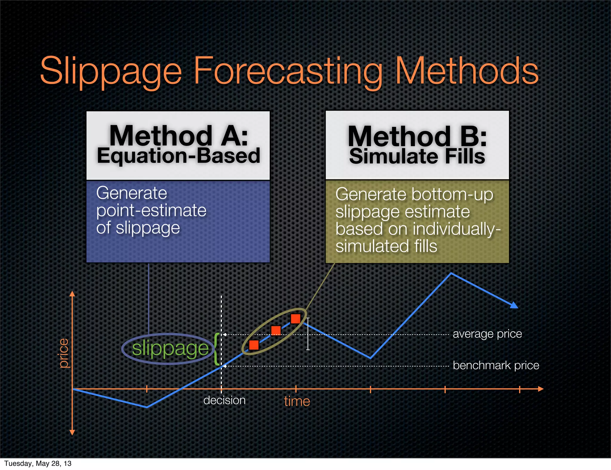
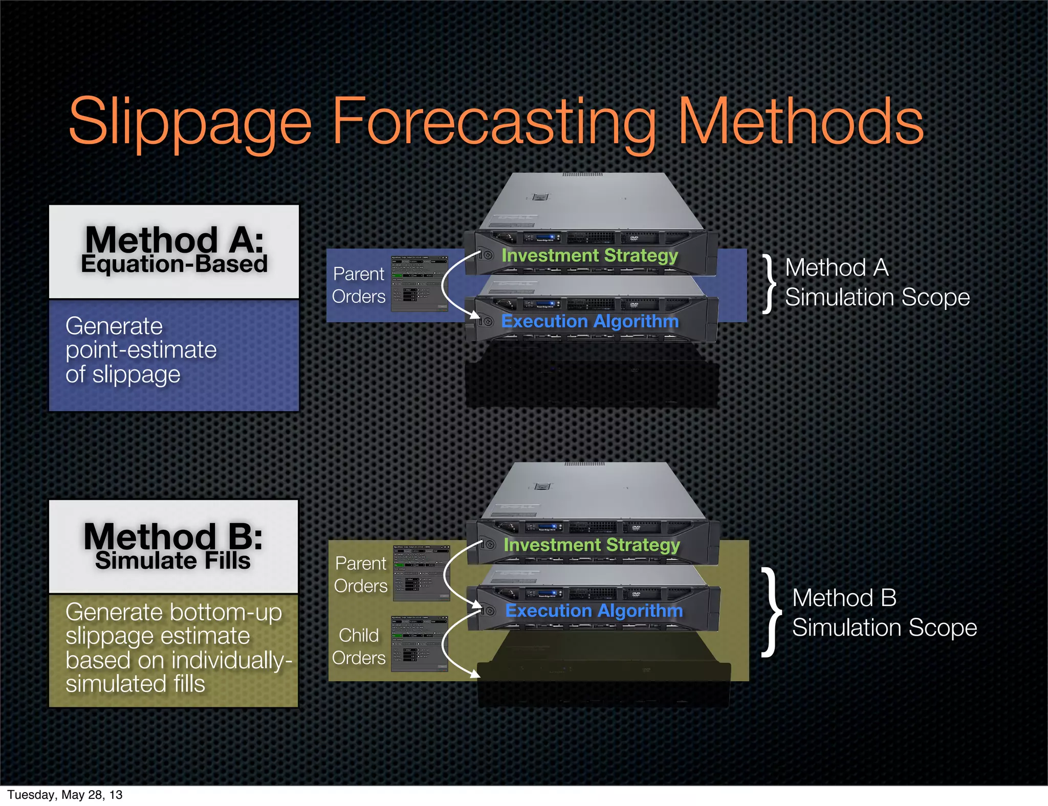
![Method A: Equation-Based
Avg Price = Baseline Price +/- [ f(spread) + g(size,...) ]
Last Price
Next Price
Bid-Ask Midpoint
Baseline
Price
✓
4 bps
f(typical spread)
f(starting spread)
f(TWA spread)
Spread
Cost
✓
✓
0
g(size, horizon,
volume, volatility)
Impact
✓
Horizon Close
Horizon VWAP
Horizon TWA-Mid
✓
✓
✓
[basic f( ) = 0.5 x spread]
Tuesday, May 28, 13](https://image.slidesharecdn.com/quantopianwebinarversion-tombok-130618142029-phpapp01/75/Modeling-Transaction-Costs-for-Algorithmic-Strategies-10-2048.jpg)
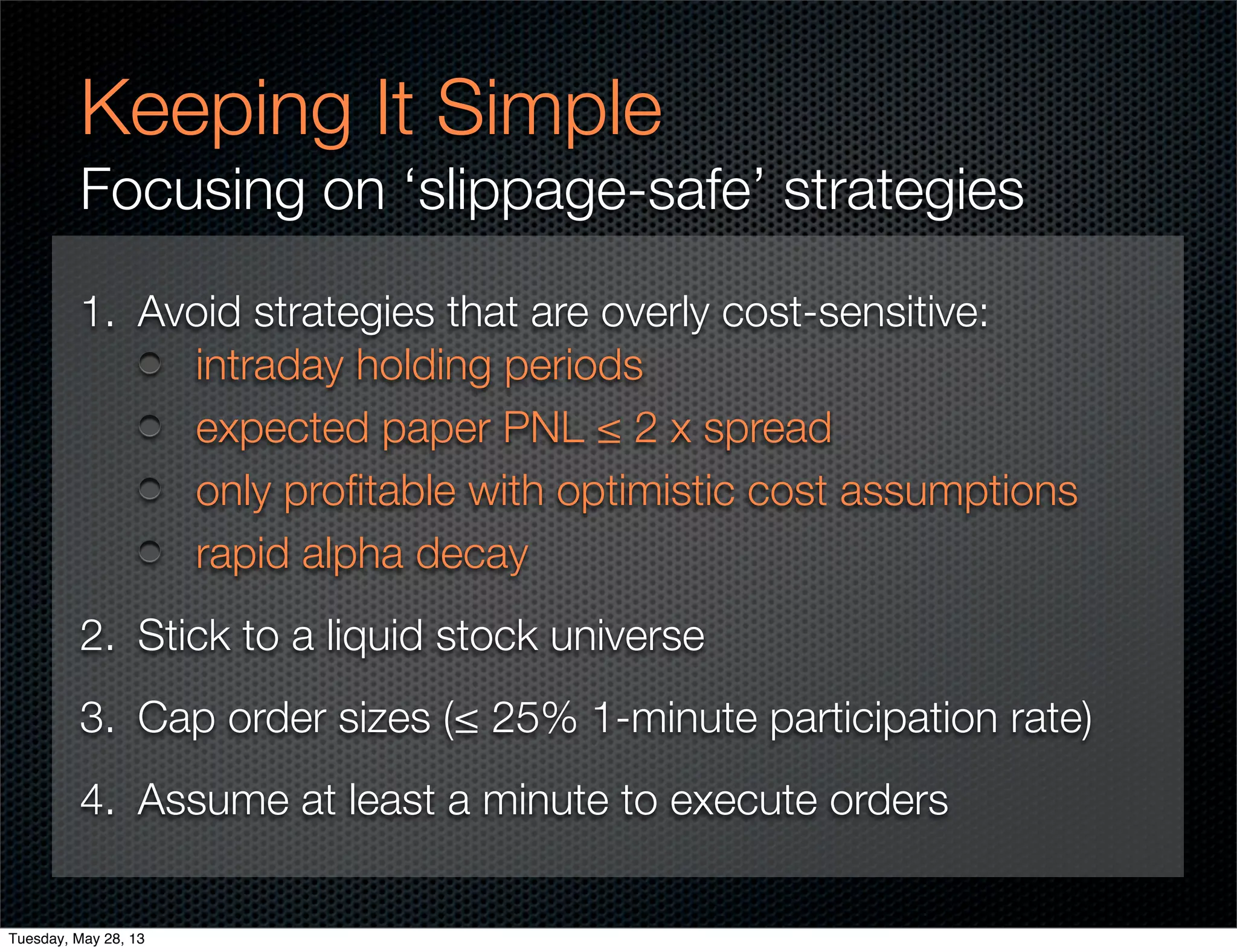

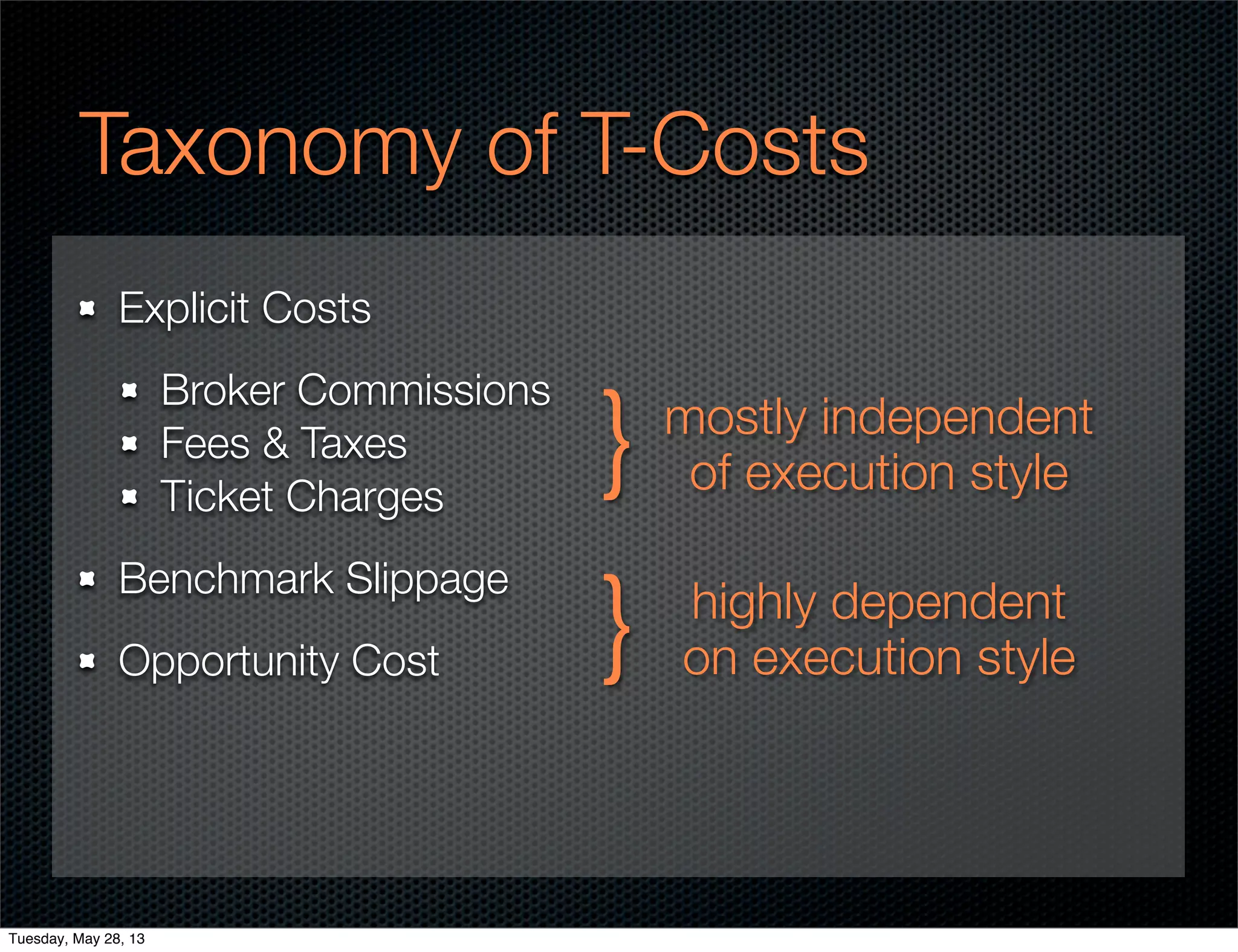
This document discusses modeling transaction costs for algorithmic trading strategies. It presents a taxonomy of explicit costs like commissions, fees, and taxes as well as opportunity costs and benchmark slippage. Two methods are described for estimating slippage: equation-based models and simulating child order fills. The appropriate method depends on the strategy's timescale. The document provides guidelines for keeping transaction cost modeling simple while still accounting for costs accurately. It emphasizes considering costs early in the strategy development process.


