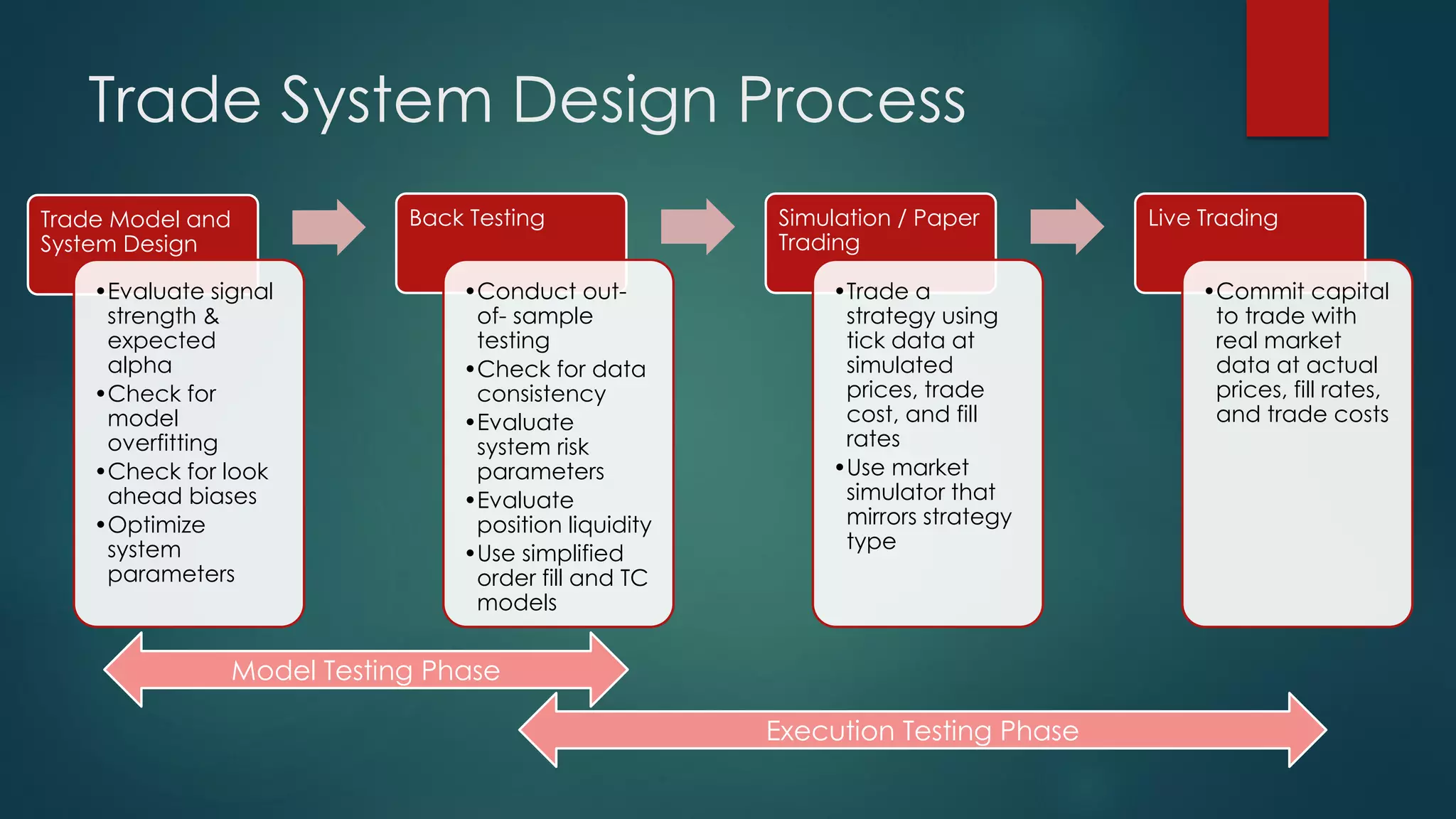
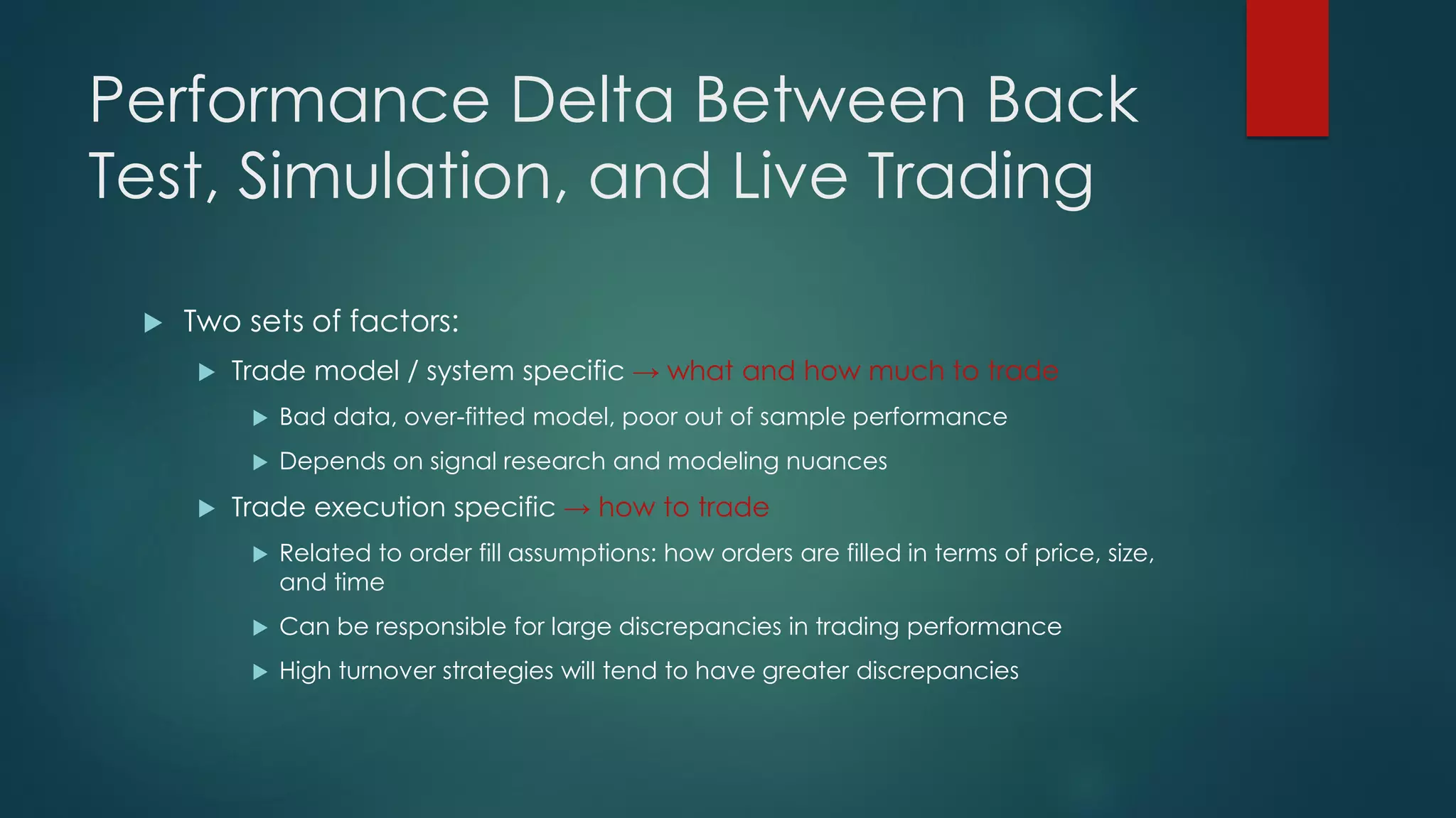
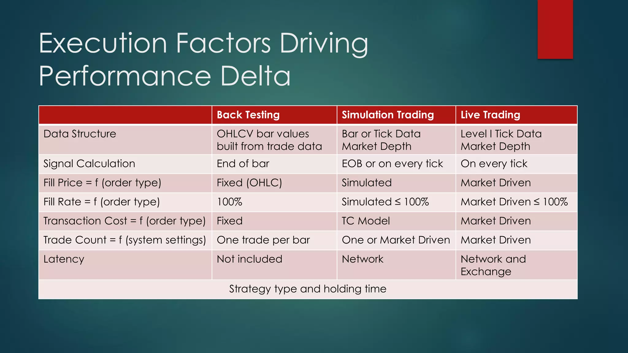
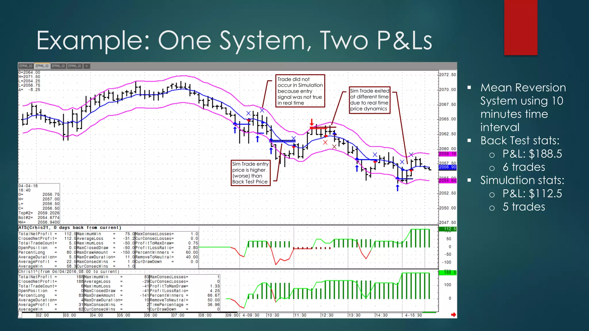
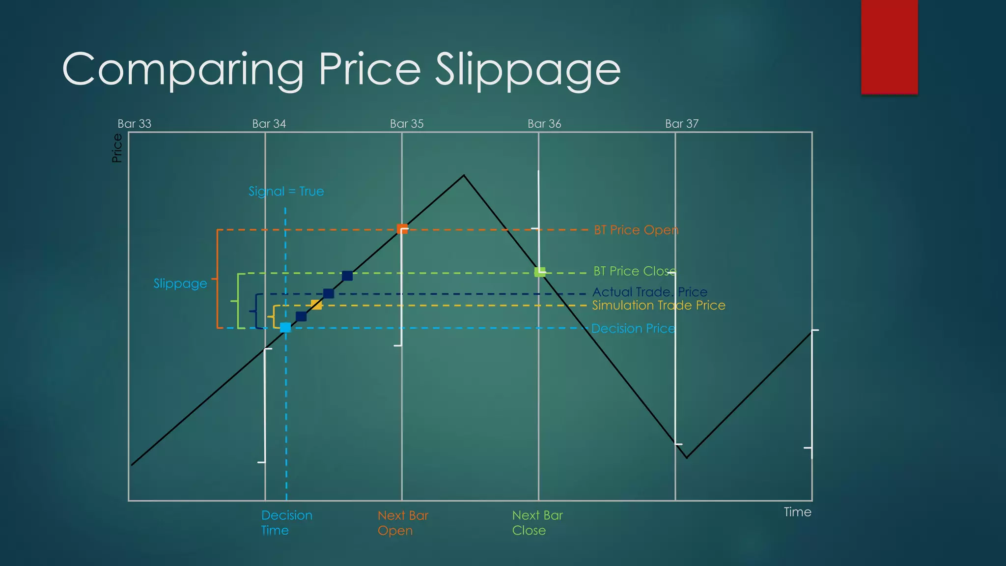
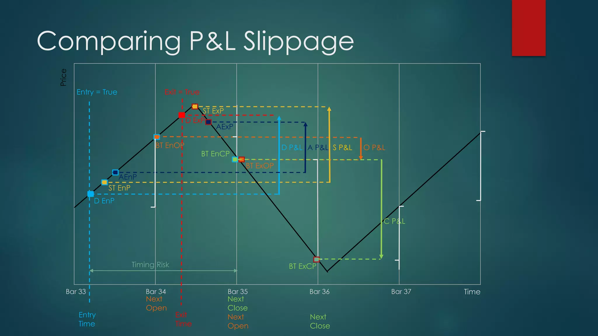
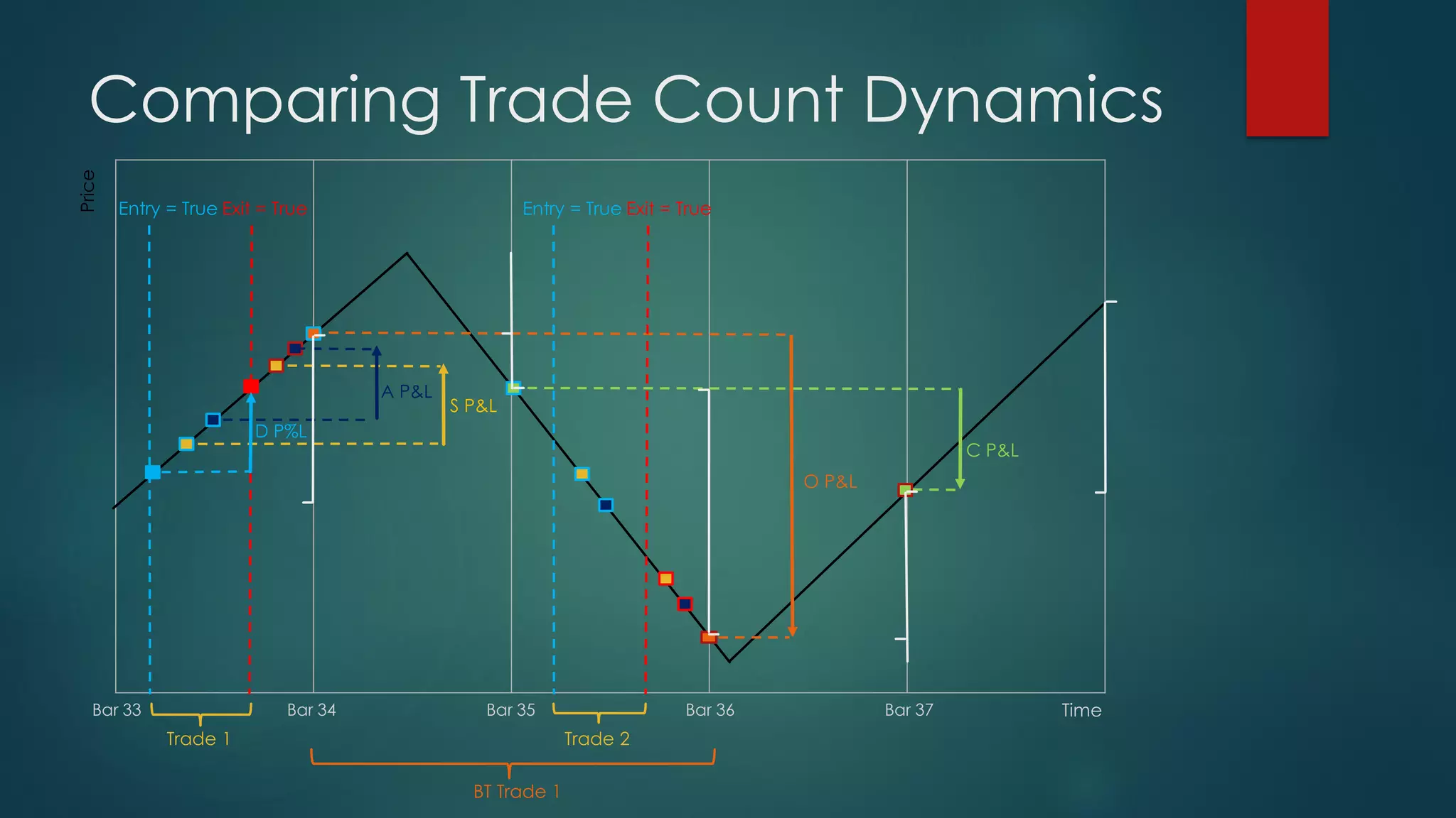
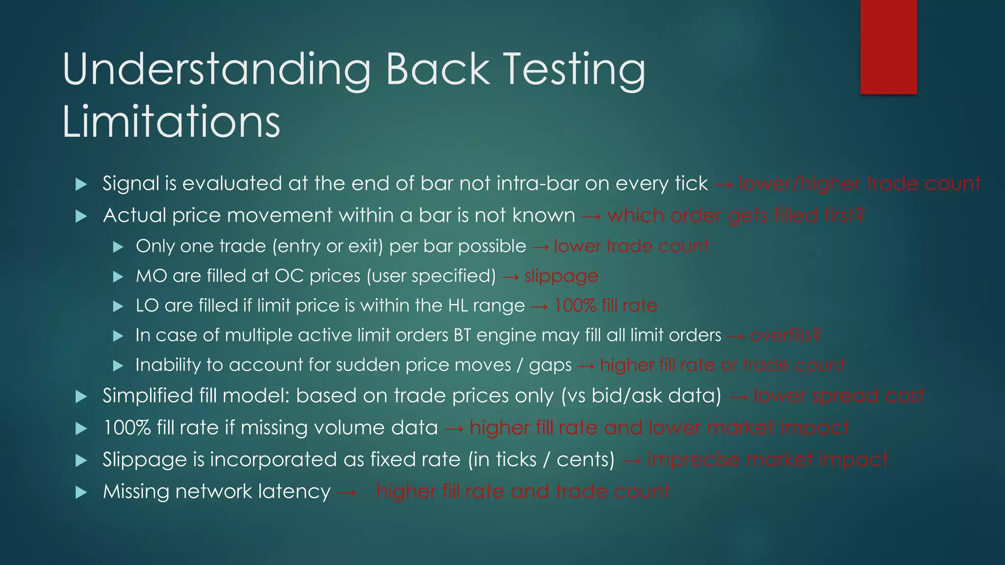
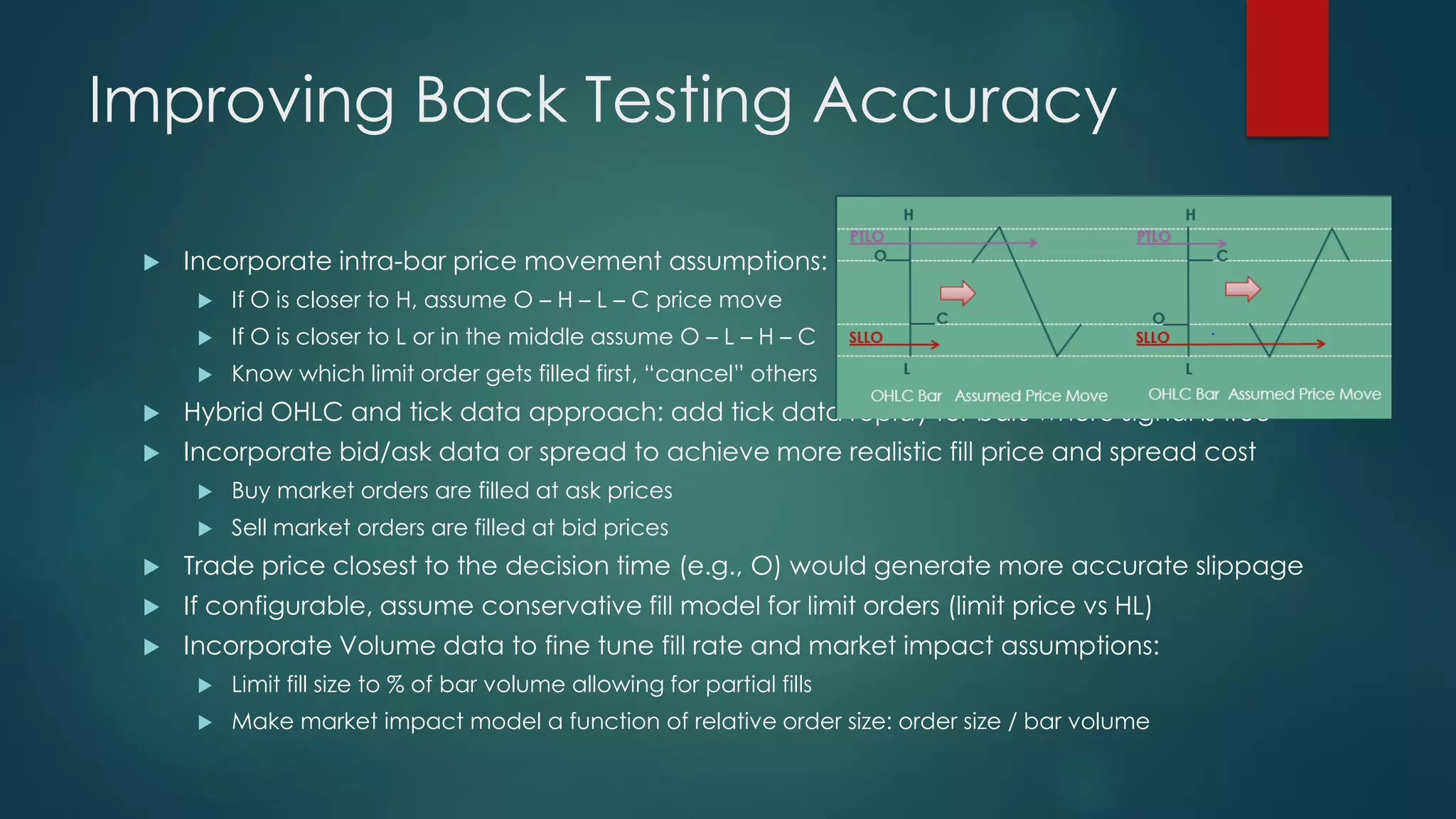
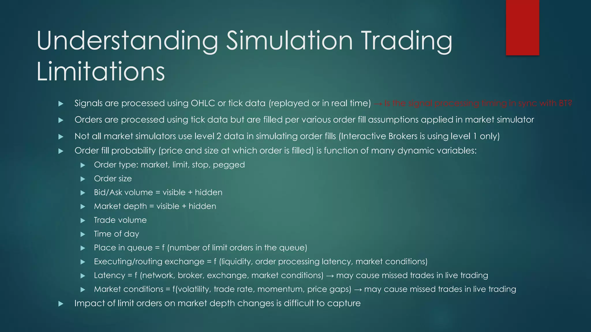
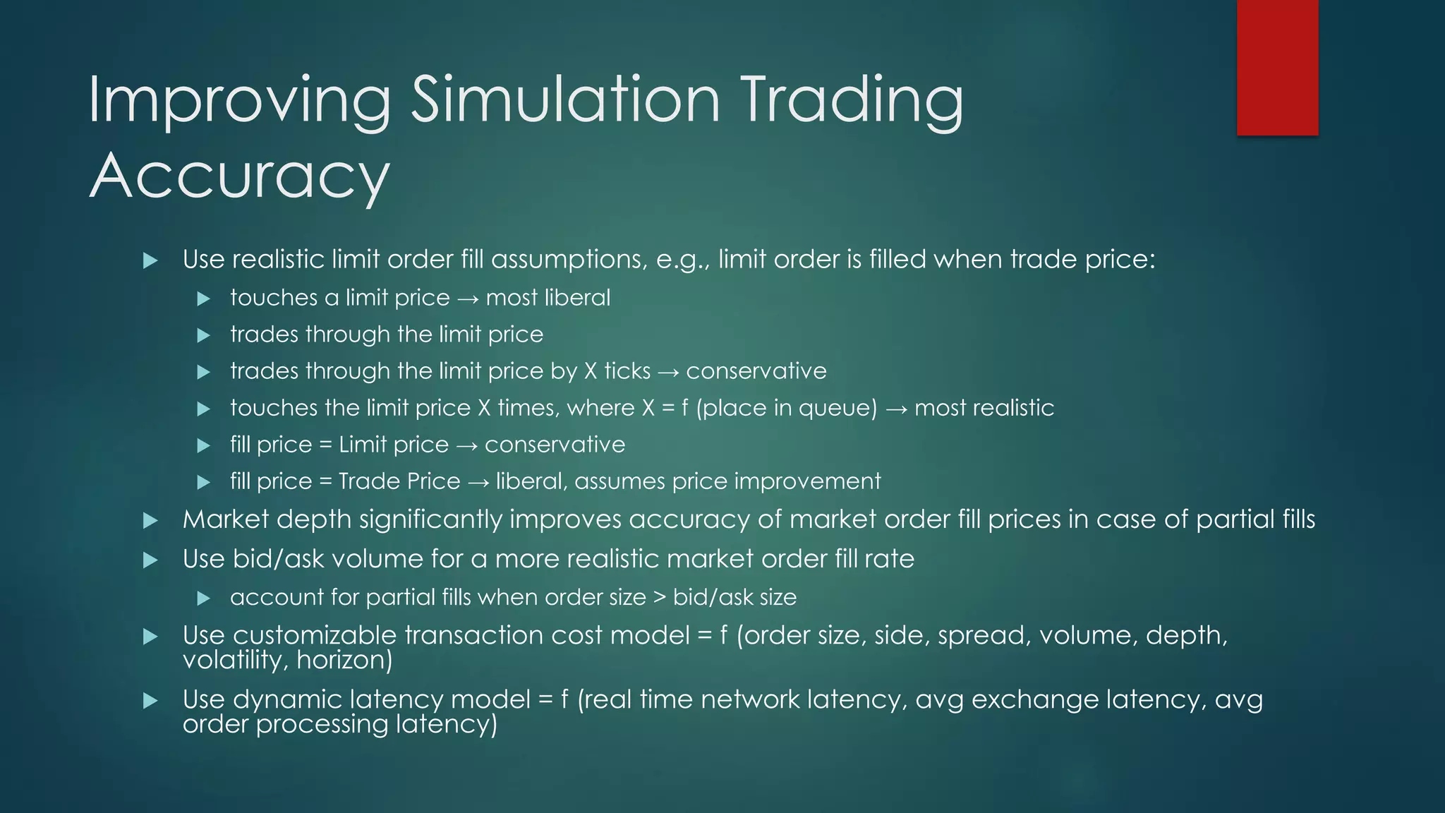
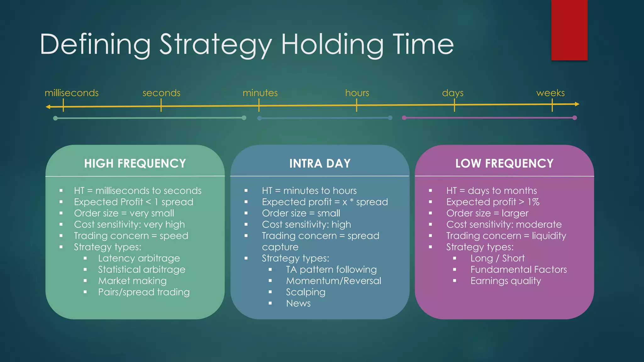
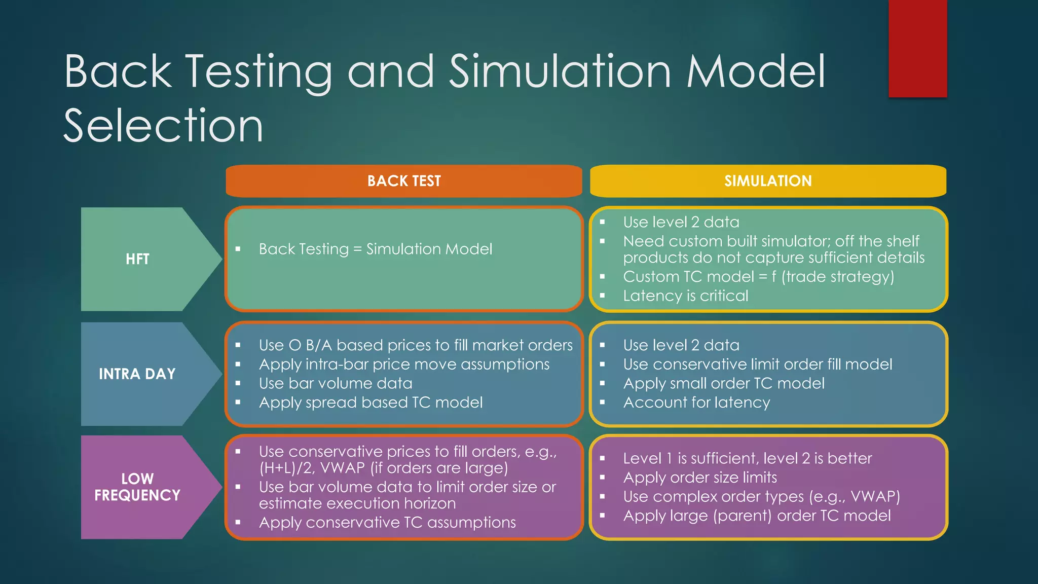
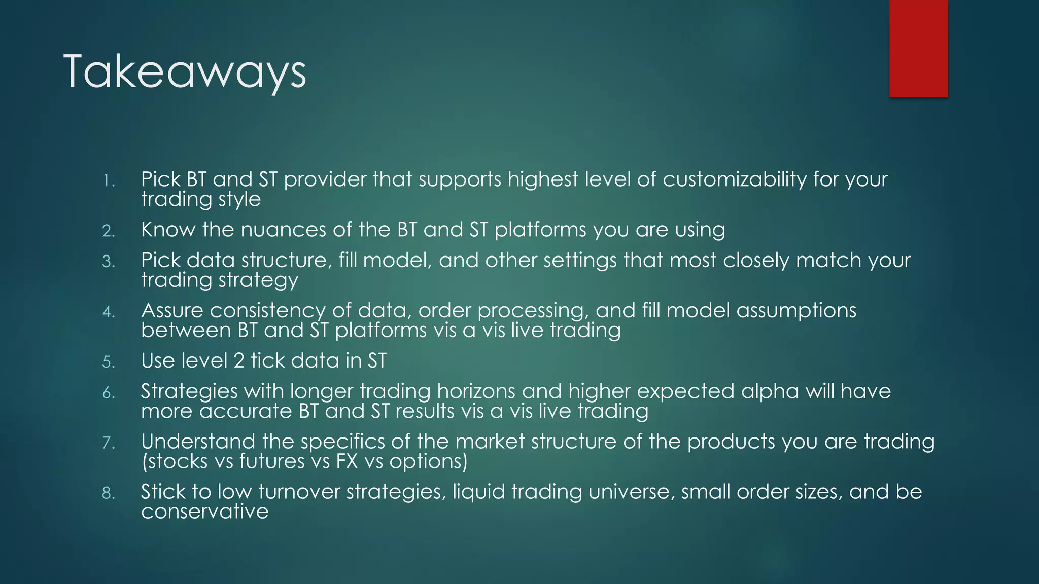
The document outlines the process of transitioning from back testing to live trading for trading systems, covering model design, execution testing, and performance evaluation. It highlights the importance of aligning back testing and simulation parameters with live trading conditions to minimize discrepancies in trading performance. Additionally, it discusses limitations and strategies for improving the accuracy of back testing and simulation, including data consistency, order fill assumptions, and market conditions.

1. From Back Testing to Live Trading
Vesna Straser, PhD
QuantCon, April 2016

2. Trade System Design Process
Trade Model and
System Design
•Evaluate signal
strength &
expected
alpha
•Check for
model
overfitting
•Check for look
ahead biases
•Optimize
system
parameters
Back Testing
•Conduct out-
of- sample
testing
•Check for data
consistency
•Evaluate
system risk
parameters
•Evaluate
position liquidity
•Use simplified
order fill and TC
models
Simulation / Paper
Trading
•Trade a
strategy using
tick data at
simulated
prices, trade
cost, and fill
rates
•Use market
simulator that
mirrors strategy
type
Live Trading
•Commit capital
to trade with
real market
data at actual
prices, fill rates,
and trade costs
Execution Testing Phase
Model Testing Phase

3. Performance Delta Between Back
Test, Simulation, and Live Trading
 Two sets of factors:
 Trade model / system specific → what and how much to trade
 Bad data, over-fitted model, poor out of sample performance
 Depends on signal research and modeling nuances
 Trade execution specific → how to trade
 Related to order fill assumptions: how orders are filled in terms of price, size,
and time
 Can be responsible for large discrepancies in trading performance
 High turnover strategies will tend to have greater discrepancies

4. Execution Factors Driving
Performance Delta
Back Testing Simulation Trading Live Trading
Data Structure OHLCV bar values
built from trade data
Bar or Tick Data
Market Depth
Level I Tick Data
Market Depth
Signal Calculation End of bar EOB or on every tick On every tick
Fill Price = f (order type) Fixed (OHLC) Simulated Market Driven
Fill Rate = f (order type) 100% Simulated ≤ 100% Market Driven ≤ 100%
Transaction Cost = f (order type) Fixed TC Model Market Driven
Trade Count = f (system settings) One trade per bar One or Market Driven Market Driven
Latency Not included Network Network and
Exchange
Strategy type and holding time

5. Example: One System, Two P&Ls
 Mean Reversion
System using 10
minutes time
interval
 Back Test stats:
o P&L: $188.5
o 6 trades
 Simulation stats:
o P&L: $112.5
o 5 trades
Trade did not
occur in Simulation
because entry
signal was not true
in real time
Sim Trade exited
at different time
due to real time
price dynamics
Sim Trade entry
price is higher
(worse) than
Back Test Price

6. Comparing Price Slippage
Actual Trade. Price
Decision Price
Simulation Trade Price
Slippage
Signal = True
Decision
Time
Price
TimeNext Bar
Open
BT Price Open
BT Price Close
Next Bar
Close
Bar 33 Bar 34 Bar 35 Bar 36 Bar 37

7. Comparing P&L Slippage
Next
Open
Entry
Time
Time
Next
Close
Next
Open
Next
Close
BT EnOP
BT EnCP
AEnP
ST EnP
Entry = True
Price
D EnP
BT ExOP
O P&L
ST ExP
S P&L
BT ExCP
C P&L
Exit
Time
Exit = True
D ExP
D P&L
Bar 33 Bar 34 Bar 35 Bar 36 Bar 37
AExP
A P&L
Timing Risk

8. Comparing Trade Count DynamicsPrice
Time
S P&L
Bar 33 Bar 34 Bar 35 Bar 36 Bar 37
A P&L
O P&L
C P&L
Exit = True
Trade 1
BT Trade 1
Entry = True Exit = True
D P%L
Entry = True
Trade 2

9. Understanding Back Testing
Limitations
 Signal is evaluated at the end of bar not intra-bar on every tick → lower/higher trade count
 Actual price movement within a bar is not known → which order gets filled first?
 Only one trade (entry or exit) per bar possible → lower trade count
 MO are filled at OC prices (user specified) → slippage
 LO are filled if limit price is within the HL range → 100% fill rate
 In case of multiple active limit orders BT engine may fill all limit orders → overfills?
 Inability to account for sudden price moves / gaps → higher fill rate or trade count
 Simplified fill model: based on trade prices only (vs bid/ask data) → lower spread cost
 100% fill rate if missing volume data → higher fill rate and lower market impact
 Slippage is incorporated as fixed rate (in ticks / cents) → imprecise market impact
 Missing network latency → higher fill rate and trade count

10. Improving Back Testing Accuracy
 Incorporate intra-bar price movement assumptions:
 If O is closer to H, assume O – H – L – C price move
 If O is closer to L or in the middle assume O – L – H – C
 Know which limit order gets filled first, “cancel” others
 Hybrid OHLC and tick data approach: add tick data replay for bars where signal is true
 Incorporate bid/ask data or spread to achieve more realistic fill price and spread cost
 Buy market orders are filled at ask prices
 Sell market orders are filled at bid prices
 Trade price closest to the decision time (e.g., O) would generate more accurate slippage
 If configurable, assume conservative fill model for limit orders (limit price vs HL)
 Incorporate Volume data to fine tune fill rate and market impact assumptions:
 Limit fill size to % of bar volume allowing for partial fills
 Make market impact model a function of relative order size: order size / bar volume

11. Understanding Simulation Trading
Limitations
 Signals are processed using OHLC or tick data (replayed or in real time) → Is the signal processing timing in sync with BT?
 Orders are processed using tick data but are filled per various order fill assumptions applied in market simulator
 Not all market simulators use level 2 data in simulating order fills (Interactive Brokers is using level 1 only)
 Order fill probability (price and size at which order is filled) is function of many dynamic variables:
 Order type: market, limit, stop, pegged
 Order size
 Bid/Ask volume = visible + hidden
 Market depth = visible + hidden
 Trade volume
 Time of day
 Place in queue = f (number of limit orders in the queue)
 Executing/routing exchange = f (liquidity, order processing latency, market conditions)
 Latency = f (network, broker, exchange, market conditions) → may cause missed trades in live trading
 Market conditions = f(volatility, trade rate, momentum, price gaps) → may cause missed trades in live trading
 Impact of limit orders on market depth changes is difficult to capture

12. Improving Simulation Trading
Accuracy
 Use realistic limit order fill assumptions, e.g., limit order is filled when trade price:
 touches a limit price → most liberal
 trades through the limit price
 trades through the limit price by X ticks → conservative
 touches the limit price X times, where X = f (place in queue) → most realistic
 fill price = Limit price → conservative
 fill price = Trade Price → liberal, assumes price improvement
 Market depth significantly improves accuracy of market order fill prices in case of partial fills
 Use bid/ask volume for a more realistic market order fill rate
 account for partial fills when order size > bid/ask size
 Use customizable transaction cost model = f (order size, side, spread, volume, depth,
volatility, horizon)
 Use dynamic latency model = f (real time network latency, avg exchange latency, avg
order processing latency)

13. Defining Strategy Holding Time
milliseconds seconds minutes hours days weeks
HIGH FREQUENCY
 HT = milliseconds to seconds
 Expected Profit < 1 spread
 Order size = very small
 Cost sensitivity: very high
 Trading concern = speed
 Strategy types:
 Latency arbitrage
 Statistical arbitrage
 Market making
 Pairs/spread trading
INTRA DAY
 HT = minutes to hours
 Expected profit = x * spread
 Order size = small
 Cost sensitivity: high
 Trading concern = spread
capture
 Strategy types:
 TA pattern following
 Momentum/Reversal
 Scalping
 News
LOW FREQUENCY
 HT = days to months
 Expected profit > 1%
 Order size = larger
 Cost sensitivity: moderate
 Trading concern = liquidity
 Strategy types:
 Long / Short
 Fundamental Factors
 Earnings quality

14. Back Testing and Simulation Model
Selection
HFT
INTRA DAY
LOW
FREQUENCY
 Back Testing = Simulation Model
 Use level 2 data
 Need custom built simulator; off the shelf
products do not capture sufficient details
 Custom TC model = f (trade strategy)
 Latency is critical
 Use O B/A based prices to fill market orders
 Apply intra-bar price move assumptions
 Use bar volume data
 Apply spread based TC model
 Use level 2 data
 Use conservative limit order fill model
 Apply small order TC model
 Account for latency
 Level 1 is sufficient, level 2 is better
 Apply order size limits
 Use complex order types (e.g., VWAP)
 Apply large (parent) order TC model
 Use conservative prices to fill orders, e.g.,
(H+L)/2, VWAP (if orders are large)
 Use bar volume data to limit order size or
estimate execution horizon
 Apply conservative TC assumptions
BACK TEST SIMULATION

15. Takeaways
1. Pick BT and ST provider that supports highest level of customizability for your
trading style
2. Know the nuances of the BT and ST platforms you are using
3. Pick data structure, fill model, and other settings that most closely match your
trading strategy
4. Assure consistency of data, order processing, and fill model assumptions
between BT and ST platforms vis a vis live trading
5. Use level 2 tick data in ST
6. Strategies with longer trading horizons and higher expected alpha will have
more accurate BT and ST results vis a vis live trading
7. Understand the specifics of the market structure of the products you are trading
(stocks vs futures vs FX vs options)
8. Stick to low turnover strategies, liquid trading universe, small order sizes, and be
conservative