The document discusses sensitivity analysis in linear programming, focusing on how changes in objective function coefficients and constraint values impact the optimal solution. It covers graphical solutions, ranges of optimality for adjusting coefficients, and the implications of changes in right-hand side values on feasibility and dual values. Additionally, it exemplifies the concepts through practical applications like the case of Olympic Bike Co., demonstrating how profit values and resource constraints affect decision-making.

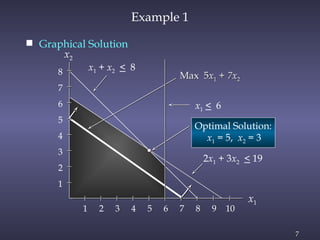
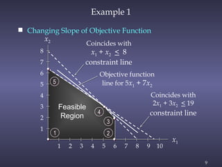
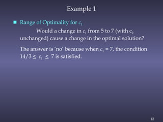
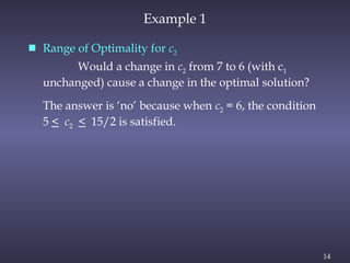
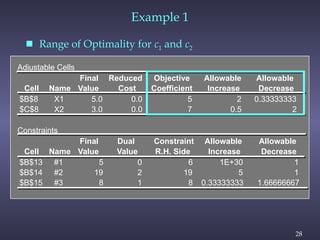
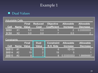
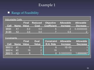
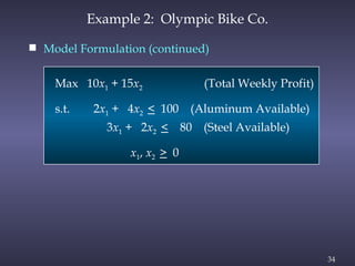
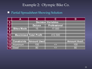
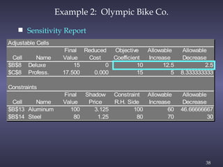
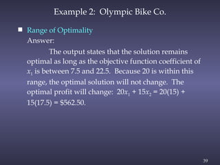
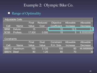
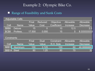
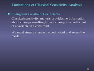
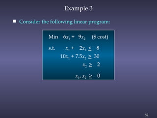
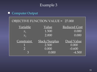
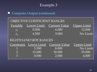
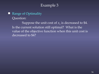
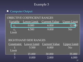
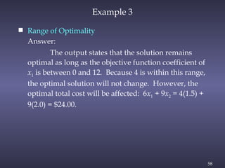
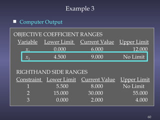
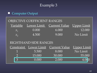
1. 1
Slides by
John
Loucks
St. Edward’s
University
Modifications by
A. Asef-Vaziri

2. 2
Chapter 3
Linear Programming: Sensitivity Analysis
and Interpretation of Solution
 Introduction to Sensitivity Analysis
 Graphical Sensitivity Analysis
 Sensitivity Analysis: Computer Solution
 Limitations of Classical Sensitivity Analysis

3. 3
 In the previous chapter we discussed:
• objective function value
• values of the decision variables
• reduced costs
• slack/surplus
 In this chapter we will discuss:
• changes in the coefficients of the objective function
• changes in the right-hand side value of a
constraint
Introduction to Sensitivity Analysis

4. 4
Introduction to Sensitivity Analysis
 Sensitivity analysis (or post-optimality analysis) is
used to determine how the optimal solution is
affected by changes, within specified ranges, in:
• the objective function coefficients
• the right-hand side (RHS) values
 Sensitivity analysis is important to a manager who
must operate in a dynamic environment with
imprecise estimates of the coefficients.
 Sensitivity analysis allows a manager to ask certain
what-if questions about the problem.

5. 5
Graphical Sensitivity Analysis
 For LP problems with two decision variables,
graphical solution methods can be used to perform
sensitivity analysis on
• the objective function coefficients, and
• the right-hand-side values for the constraints.

6. 6
Example 1
 LP Formulation
Max 5x1 + 7x2
s.t. x1 < 6
2x1 + 3x2 < 19
x1 + x2 < 8
x1, x2 > 0

7. 7
Example 1
 Graphical Solution
2x1 + 3x2 < 19
x2
x1
x1 + x2 < 8
Max 5x1 + 7x2
x1 < 6
Optimal Solution:
x1 = 5, x2 = 3
8
7
6
5
4
3
2
1
1 2 3 4 5 6 7 8 9 10

8. 8
Objective Function Coefficients
 Let us consider how changes in the objective function
coefficients might affect the optimal solution.
 The range of optimality for each coefficient provides
the range of values over which the current solution
will remain optimal.
 Managers should focus on those objective coefficients
that have a narrow range of optimality and
coefficients near the endpoints of the range.

9. 9
Example 1
 Changing Slope of Objective Function
x1
Feasible
Region
1 2
3
4
5
x2
Coincides with
x1 + x2 < 8
constraint line
8
7
6
5
4
3
2
1
1 2 3 4 5 6 7 8 9 10
Coincides with
2x1 + 3x2 < 19
constraint line
Objective function
line for 5x1 + 7x2

10. 10
Range of Optimality
 Graphically, the limits of a range of optimality are
found by changing the slope of the objective function
line within the limits of the slopes of the binding
constraint lines.
 Slope of an objective function line, Max c1x1 + c2x2, is
-c1/c2, and the slope of a constraint, a1x1 + a2x2 = b, is
-a1/a2.

11. 11
Example 1
 Range of Optimality for c1
The slope of the objective function line is
-c1/c2. The slope of the first binding constraint, x1 +
x2 = 8, is -1 and the slope of the second binding
constraint, x1 + 3x2 = 19, is -2/3.
Find the range of values for c1 (with c2 staying
7) such that the objective function line slope lies
between that of the two binding constraints:
-1 < -c1/7 < -2/3
Multiplying through by -7 (and reversing the
inequalities):
14/3 < c1 < 7

12. 12
Example 1
 Range of Optimality for c1
Would a change in c1 from 5 to 7 (with c2
unchanged) cause a change in the optimal solution?
The answer is ‘no’ because when c1 = 7, the condition
14/3 < c1 < 7 is satisfied.

13. 13
Example 1
 Range of Optimality for c2
Find the range of values for c2 ( with c1 staying
5) such that the objective function line slope lies
between that of the two binding constraints:
-1 < -5/c2 < -2/3
Multiplying by -1: 1 > 5/c2 > 2/3
Inverting, 1 < c2/5 < 3/2
Multiplying by 5: 5 < c2 < 15/2

14. 14
Example 1
 Range of Optimality for c2
Would a change in c2 from 7 to 6 (with c1
unchanged) cause a change in the optimal solution?
The answer is ‘no’ because when c2 = 6, the condition
5 < c2 < 15/2 is satisfied.

15. 15
 The range of optimality for objective function
coefficients is only applicable for changes made to one
coefficient at a time.
 All other coefficients are assumed to be fixed at their
initial values.
 If two or more coefficients are changed simultaneously,
further analysis is usually necessary.
 However, when solving two-variable problems
graphically, the analysis is fairly easy.
Simultaneous Changes

16. 16
 Simply compute the slope of the objective function
(-Cx1
/Cx2
) for the new coefficient values.
 If this ratio is > the lower limit on the slope of the
objective function and < the upper limit, then the
changes made will not cause a change in the optimal
solution.
Simultaneous Changes

17. 17
Recall that the objective function line slope
must lie between that of the two binding constraints:
-1 < -c1/c2 < -2/3
The answer is ‘yes’ the optimal solution
changes because -7/6 does not satisfy the above
condition.
Example 1
 Simultaneous Changes in c1 and c2
Would simultaneously changing c1 from 5 to 7
and changing c2 from 7 to 6 cause a change in the
optimal solution? (Recall that these changes
individually did not cause the optimal solution to
change.)

18. 18
Right-Hand Sides
 Let us consider how a change in the right-hand side
for a constraint might affect the feasible region and
perhaps cause a change in the optimal solution.
 The change in the value of the optimal solution per
unit increase in the right-hand side is called the dual
value.
 The range of feasibility is the range over which the
dual value is applicable.
 As the RHS increases, other constraints will become
binding and limit the change in the value of the
objective function.

19. 19
Dual Value
 Graphically, a dual value is determined by adding +1
to the right hand side value in question and then
resolving for the optimal solution in terms of the
same two binding constraints.
 The dual value is equal to the difference in the values
of the objective functions between the new and
original problems.
 The dual value for a nonbinding constraint is 0.
 A negative dual value indicates that the objective
function will not improve if the RHS is increased.

20. 20
Example 1
 Dual Values
Constraint 1: Since x1 < 6 is not a binding constraint,
its dual price is 0.
Constraint 2: Change the RHS value of the second
constraint to 20 and resolve for the
optimal point determined by the last two
constraints: 2x1 + 3x2 = 20 and x1 + x2 =
8.
The solution is x1 = 4, x2 = 4, z = 48. Hence,
the dual price = znew - zold = 48 - 46 = 2.

21. 21
Example 1
 Dual Values
Constraint 3: Change the RHS value of the third
constraint to 9 and resolve for the optimal point
determined by the last two constraints: 2x1 + 3x2 =
19 and x1 + x2 = 9.
The solution is: x1 = 8, x2 = 1, z = 47.
The dual price is znew - zold = 47 - 46 = 1.

22. 22
Range of Feasibility
 The range of feasibility for a change in the right hand
side value is the range of values for this coefficient in
which the original dual value remains constant.
 Graphically, the range of feasibility is determined by
finding the values of a right hand side coefficient
such that the same two lines that determined the
original optimal solution continue to determine the
optimal solution for the problem.

23. 23
Software packages such as Lingo and Microsoft Excel
provide the following LP information:
 Information about the objective function:
• its optimal value
• coefficient ranges (ranges of optimality)
 Information about the decision variables:
• their optimal values
• their reduced costs
 Information about the constraints:
• the amount of slack or surplus
• the dual prices
• right-hand side ranges (ranges of feasibility)
Sensitivity Analysis: Computer Solution

24. 24
 The reduced cost associated with a variable is equal
to the dual value for the non-negativity constraint
associated with the variable.
 In general, if a variable has a non-zero value in the
optimal solution, then it will have a reduced cost
equal to 0.
Reduced Cost

25. 25
Relevant Cost and Sunk Cost
 A resource cost is a relevant cost if the amount paid
for it is dependent upon the amount of the resource
used by the decision variables.
 Relevant costs are reflected in the objective function
coefficients.
 A resource cost is a sunk cost if it must be paid
regardless of the amount of the resource actually
used by the decision variables.
 Sunk resource costs are not reflected in the objective
function coefficients.

26. 26
Cautionary Note on
the Interpretation of Dual Values
 Resource cost is sunk
The dual value is the maximum amount you should
be willing to pay for one additional unit of the
resource.
 Resource cost is relevant
The dual value is the maximum premium over the
normal cost that you should be willing to pay for one
unit of the resource.

27. 27
Example 1 (Again)
 LP Formulation
Max 5x1 + 7x2
s.t. x1 < 6
2x1 + 3x2 < 19
x1 + x2 < 8
x1, x2 > 0

28. 28
Example 1
 Range of Optimality for c1 and c2
Adjustable Cells
Final Reduced Objective Allowable Allowable
Cell Name Value Cost Coefficient Increase Decrease
$B$8 X1 5.0 0.0 5 2 0.33333333
$C$8 X2 3.0 0.0 7 0.5 2
Constraints
Final Dual Constraint Allowable Allowable
Cell Name Value Value R.H. Side Increase Decrease
$B$13 #1 5 0 6 1E+30 1
$B$14 #2 19 2 19 5 1
$B$15 #3 8 1 8 0.33333333 1.66666667

29. 29
Example 1
 Dual Values
Adjustable Cells
Final Reduced Objective Allowable Allowable
Cell Name Value Cost Coefficient Increase Decrease
$B$8 X1 5.0 0.0 5 2 0.33333333
$C$8 X2 3.0 0.0 7 0.5 2
Constraints
Final Dual Constraint Allowable Allowable
Cell Name Value Value R.H. Side Increase Decrease
$B$13 #1 5 0 6 1E+30 1
$B$14 #2 19 2 19 5 1
$B$15 #3 8 1 8 0.33333333 1.66666667

30. 30
Example 1
 Range of Feasibility
Adjustable Cells
Final Reduced Objective Allowable Allowable
Cell Name Value Cost Coefficient Increase Decrease
$B$8 X1 5.0 0.0 5 2 0.33333333
$C$8 X2 3.0 0.0 7 0.5 2
Constraints
Final Dual Constraint Allowable Allowable
Cell Name Value Value R.H. Side Increase Decrease
$B$13 #1 5 0 6 1E+30 1
$B$14 #2 19 2 19 5 1
$B$15 #3 8 1 8 0.33333333 1.66666667

31. 31
Olympic Bike is introducing two new lightweight
bicycle frames, the Deluxe and the Professional, to be
made from special aluminum and steel alloys. The
anticipated unit profits are $10 for the Deluxe and $15
for the Professional.
The number of pounds of each alloy needed per
frame is summarized on the next slide.
Example 2: Olympic Bike Co.

32. 32
A supplier delivers 100 pounds of the aluminum
alloy and 80 pounds of the steel alloy weekly.
Aluminum Alloy Steel Alloy
Deluxe 2 3
Professional 4 2
How many Deluxe and Professional frames
should
Olympic produce each week?
Example 2: Olympic Bike Co.

33. 33
Example 2: Olympic Bike Co.
 Model Formulation
• Verbal Statement of the Objective Function
Maximize total weekly profit.
• Verbal Statement of the Constraints
Total weekly usage of aluminum alloy < 100 pounds.
Total weekly usage of steel alloy < 80 pounds.
• Definition of the Decision Variables
x1 = number of Deluxe frames produced weekly.
x2 = number of Professional frames produced weekly.

34. 34
Example 2: Olympic Bike Co.
 Model Formulation (continued)
Max 10x1 + 15x2 (Total Weekly Profit)
s.t. 2x1 + 4x2 < 100 (Aluminum Available)
3x1 + 2x2 < 80 (Steel Available)
x1, x2 > 0

35. 35
Example 2: Olympic Bike Co.
 Partial Spreadsheet Showing Solution
A B C D
6
7 Deluxe Professional
8 Bikes Made 15 17.500
9
10 412.500
11
12 Constraints Amount Used Amount Avail.
13 Aluminum 100 <= 100
14 Steel 80 <= 80
Decision Variables
Maximized Total Profit
A B C D
6
7 Deluxe Professional
8 Bikes Made 15 17.500
9
10 412.500
11
12 Constraints Amount Used Amount Avail.
13 Aluminum 100 <= 100
14 Steel 80 <= 80
Decision Variables
Maximized Total Profit

36. 36
Example 2: Olympic Bike Co.
 Optimal Solution
According to the output:
x1 (Deluxe frames) = 15
x2 (Professional frames) = 17.5
Objective function value = $412.50

37. 37
Example 2: Olympic Bike Co.
 Range of Optimality
Question:
Suppose the profit on deluxe frames is
increased to $20. Is the above solution still optimal?
What is the value of the objective function when this
unit profit is increased to $20?

38. 38
Example 2: Olympic Bike Co.
 Sensitivity Report
Adjustable Cells
Final Reduced Objective Allowable Allowable
Cell Name Value Cost Coefficient Increase Decrease
$B$8 Deluxe 15 0 10 12.5 2.5
$C$8 Profess. 17.500 0.000 15 5 8.333333333
Constraints
Final Shadow Constraint Allowable Allowable
Cell Name Value Price R.H. Side Increase Decrease
$B$13 Aluminum 100 3.125 100 60 46.66666667
$B$14 Steel 80 1.25 80 70 30

39. 39
Example 2: Olympic Bike Co.
 Range of Optimality
Answer:
The output states that the solution remains
optimal as long as the objective function coefficient of
x1 is between 7.5 and 22.5. Because 20 is within this
range, the optimal solution will not change. The
optimal profit will change: 20x1 + 15x2 = 20(15) +
15(17.5) = $562.50.

40. 40
Example 2: Olympic Bike Co.
 Range of Optimality
Question:
If the unit profit on deluxe frames were $6
instead of $10, would the optimal solution change?

41. 41
Example 2: Olympic Bike Co.
 Range of Optimality
Adjustable Cells
Final Reduced Objective Allowable Allowable
Cell Name Value Cost Coefficient Increase Decrease
$B$8 Deluxe 15 0 10 12.5 2.5
$C$8 Profess. 17.500 0.000 15 5 8.333333333
Constraints
Final Dual Constraint Allowable Allowable
Cell Name Value Value R.H. Side Increase Decrease
$B$13 Aluminum 100 3.125 100 60 46.66666667
$B$14 Steel 80 1.25 80 70 30

42. 42
 Range of Optimality
Answer:
The output states that the solution remains
optimal as long as the objective function coefficient of
x1 is between 7.5 and 22.5. Because 6 is outside this
range, the optimal solution would change.
Example 2: Olympic Bike Co.

43. 43
Example 2: Olympic Bike Co.
 Range of Feasibility and Sunk Costs
Question:
Given that aluminum is a sunk cost, what is
the maximum amount the company should pay for
50 extra pounds of aluminum?

44. 44
Example 2: Olympic Bike Co.
 Range of Feasibility and Sunk Costs
Adjustable Cells
Final Reduced Objective Allowable Allowable
Cell Name Value Cost Coefficient Increase Decrease
$B$8 Deluxe 15 0 10 12.5 2.5
$C$8 Profess. 17.500 0.000 15 5 8.333333333
Constraints
Final Dual Constraint Allowable Allowable
Cell Name Value Value R.H. Side Increase Decrease
$B$13 Aluminum 100 3.125 100 60 46.66666667
$B$14 Steel 80 1.25 80 70 30

45. 45
Example 2: Olympic Bike Co.
 Range of Feasibility and Sunk Costs
Answer:
Because the cost for aluminum is a sunk cost,
the shadow price provides the value of extra
aluminum. The shadow price for aluminum is the
same as its dual value (for a maximization problem).
The shadow price for aluminum is $3.125 per pound
and the maximum allowable increase is 60 pounds.
Because 50 is in this range, the $3.125 is valid. Thus,
the value of 50 additional pounds is = 50($3.125) =
$156.25.

46. 46
Example 2: Olympic Bike Co.
 Range of Feasibility and Relevant Costs
Question:
If aluminum were a relevant cost, what is the
maximum amount the company should pay for 50
extra pounds of aluminum?

47. 47
Example 2: Olympic Bike Co.
 Range of Feasibility and Relevant Costs
Answer:
If aluminum were a relevant cost, the shadow
price would be the amount above the normal price of
aluminum the company would be willing to pay.
Thus if initially aluminum cost $4 per pound, then
additional units in the range of feasibility would be
worth $4 + $3.125 = $7.125 per pound.

48. 48
Limitations of Classical Sensitivity Analysis
 Classical sensitivity analysis provided by most
computer packages does have its limitations.
 It is rarely the case that one solves a model once and
makes recommendations.
 More often, a series of models is solved using a
variety of input data sets before a final plan is
adopted.

49. 49
Limitations of Classical Sensitivity Analysis
 Simultaneous Changes
The range analysis for objective function coefficients
and the constraint right-hand sides is only applicable
for changes in a single coefficient.
We should resolve the model with the new coefficient
values.

50. 50
Limitations of Classical Sensitivity Analysis
 Changes in Constraint Coefficients
Classical sensitivity analysis provides no information
about changes resulting from a change in a coefficient
of a variable in a constraint.
We must simply change the coefficient and rerun the
model.

51. 51
Limitations of Classical Sensitivity Analysis
 Non-intuitive Dual Values
Constraints with variables naturally on both the left-
hand and right-hand sides often lead to dual values
that have a non-intuitive explanation.
This is often the case with constraints that involve
percentages.
The model should be resolved with the new
percentages.

52. 52
Example 3
 Consider the following linear program:
Min 6x1 + 9x2 ($ cost)
s.t. x1 + 2x2 < 8
10x1 + 7.5x2 > 30
x2 > 2
x1, x2 > 0

53. 53
Example 3
 Computer Output
OBJECTIVE FUNCTION VALUE = 27.000
Variable Value Reduced Cost
x1 1.500 0.000
x2 2.000 0.000
Constraint Slack/Surplus Dual Value
1 2.500 0.000
2 0.000 -0.600
3 0.000 -4.500

54. 54
Example 3
 Computer Output (continued)
OBJECTIVE COEFFICIENT RANGES
Variable Lower Limit Current Value Upper Limit
x1 0.000 6.000 12.000
x2 4.500 9.000 No Limit
RIGHTHAND SIDE RANGES
Constraint Lower Limit Current Value Upper Limit
1 5.500 8.000 No Limit
2 15.000 30.000 55.000
3 0.000 2.000 4.000

55. 55
Example 3
 Optimal Solution
According to the output:
x1 = 1.5
x2 = 2.0
Objective function value = 27.00

56. 56
Example 3
 Range of Optimality
Question:
Suppose the unit cost of x1 is decreased to $4.
Is the current solution still optimal? What is the
value of the objective function when this unit cost is
decreased to $4?

57. 57
Example 3
 Computer Output
OBJECTIVE COEFFICIENT RANGES
Variable Lower Limit Current Value Upper Limit
x1 0.000 6.000 12.000
x2 4.500 9.000 No
Limit
RIGHTHAND SIDE RANGES
Constraint Lower Limit Current Value Upper Limit
1 5.500 8.000 No
Limit
2 15.000 30.000 55.000
3 0.000 2.000 4.000

58. 58
Example 3
 Range of Optimality
Answer:
The output states that the solution remains
optimal as long as the objective function coefficient of
x1 is between 0 and 12. Because 4 is within this range,
the optimal solution will not change. However, the
optimal total cost will be affected: 6x1 + 9x2 = 4(1.5) +
9(2.0) = $24.00.

59. 59
Example 3
 Range of Optimality
Question:
How much can the unit cost of x2 be decreased
without concern for the optimal solution changing?

60. 60
Example 3
 Computer Output
OBJECTIVE COEFFICIENT RANGES
Variable Lower Limit Current Value Upper Limit
x1 0.000 6.000 12.000
x2 4.500 9.000 No Limit
RIGHTHAND SIDE RANGES
Constraint Lower Limit Current Value Upper Limit
1 5.500 8.000 No Limit
2 15.000 30.000 55.000
3 0.000 2.000 4.000

61. 61
Example 3
 Range of Optimality
Answer:
The output states that the solution remains
optimal as long as the objective function coefficient of
x2 does not fall below 4.5.

62. 62
Example 3
 Range of Feasibility
Question:
If the right-hand side of constraint 3 is
increased by 1, what will be the effect on the optimal
solution?

63. 63
Example 3
 Computer Output
OBJECTIVE COEFFICIENT RANGES
Variable Lower Limit Current Value Upper Limit
x1 0.000 6.000 12.000
x2 4.500 9.000 No Limit
RIGHTHAND SIDE RANGES
Constraint Lower Limit Current Value Upper Limit
1 5.500 8.000 No Limit
2 15.000 30.000 55.000
3 0.000 2.000 4.000

64. 64
Example 3
 Range of Feasibility
Answer:
A dual value represents the improvement in
the objective function value per unit increase in the
right-hand side. A negative dual value indicates a
deterioration (negative improvement) in the
objective, which in this problem means an increase in
total cost because we're minimizing. Since the right-
hand side remains within the range of feasibility,
there is no change in the optimal solution. However,
the objective function value increases by $4.50.

65. 65
End of Chapter 3