Download as PDF, PPTX
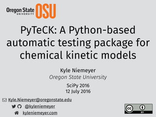


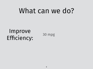

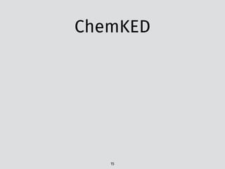
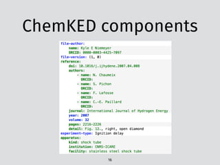
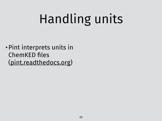
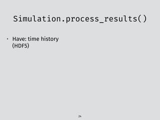
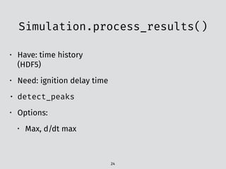
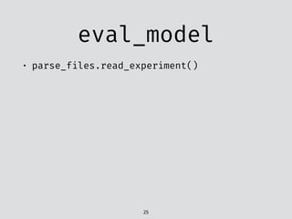
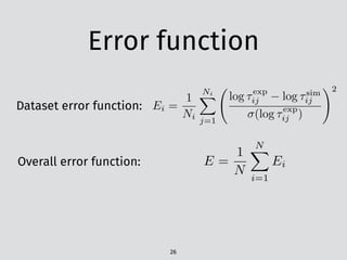
![The problem:
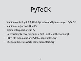
experimental data
12
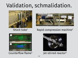
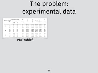
PDF table5
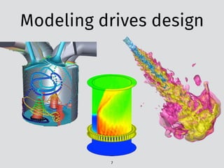
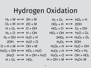
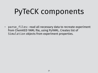
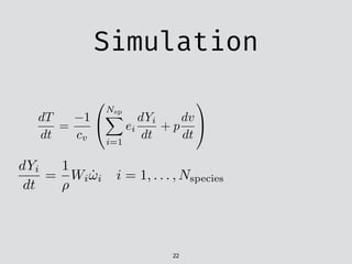
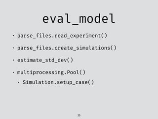
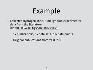
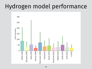
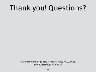
t [ms3 ~- metric benzene-air mixture.
region the dependence of the ignition delay
time upon temperature can be expressed ap-
proximately by straight lines in the Arrhenius
plot. The corresponding global activation ener-
gies decrease with increasing pressure.
For Ps around 13.5 bar the dependence be-
comes strongly nonlinear in a temperature
range between 950 and 700 K. In this interme-
diate temperature region a decrease in ignition
delay time is observed with decreasing temper-
atures. This leads to an S-shaped curve with a
maximum and a minimum. Between both ex-
termal values the dependence possesses a neg-
ative temperature coefficient. The position of
this transition region shifts to higher tempera-
tures with increasing pressures Ps- In the low-
temperature region--below approximately 700
K--the dependence of the ignition delay time
upon temperature can again be expressed by a
linear dependence. Because the measuring time
of the shock tube is limited, the delay times
could be determined only above 660 K, so that
only a short part of the low-temperature region
could be investigated in our experiments. The
influence of pressure on the ignition delay is
most pronounced in the transition region,
smallest for low temperatures and of varying
degree in the high-temperature region, where
with increasing temperature this dependence
becomes smaller.
"1~z
[ms]
101
100
1o-1
162
,, 3.2bar ,,./--~-~.~ /.-'~
o 6.s ,, ./ '---J.//
O I£3 " / ' / n [] ..~-/
30 ,,,, .o
,~_ D,,- x i< 3 bar 1 Comoufofion
~o/"°E~/" × ~+.---+-.---L_._.+_.~..~" ~ X13 " ,, [ , " ,
t/~ / /" !.ine of /+0 " j el'. a[.
/.z~ ~/ ./ pressure variation
,/~// T=9/,0 K (Fig.11) T
/ 1200 1000 800 [K]
I I I i I I I I I l I
0:8 1.o 1.2 114 loooK
T
Fig. 3. Ignition delay times.
Figure6](https://image.slidesharecdn.com/scipy2016-pyteck-160713162513/85/PyTeCK-A-Python-based-automatic-testing-package-for-chemical-kinetic-models-30-320.jpg)
![The problem:
experimental data
12
PDF table5
t [ms3 ~- metric benzene-air mixture.
region the dependence of the ignition delay
time upon temperature can be expressed ap-
proximately by straight lines in the Arrhenius
plot. The corresponding global activation ener-
gies decrease with increasing pressure.
For Ps around 13.5 bar the dependence be-
comes strongly nonlinear in a temperature
range between 950 and 700 K. In this interme-
diate temperature region a decrease in ignition
delay time is observed with decreasing temper-
atures. This leads to an S-shaped curve with a
maximum and a minimum. Between both ex-
termal values the dependence possesses a neg-
ative temperature coefficient. The position of
this transition region shifts to higher tempera-
tures with increasing pressures Ps- In the low-
temperature region--below approximately 700
K--the dependence of the ignition delay time
upon temperature can again be expressed by a
linear dependence. Because the measuring time
of the shock tube is limited, the delay times
could be determined only above 660 K, so that
only a short part of the low-temperature region
could be investigated in our experiments. The
influence of pressure on the ignition delay is
most pronounced in the transition region,
smallest for low temperatures and of varying
degree in the high-temperature region, where
with increasing temperature this dependence
becomes smaller.
"1~z
[ms]
101
100
1o-1
162
,, 3.2bar ,,./--~-~.~ /.-'~
o 6.s ,, ./ '---J.//
O I£3 " / ' / n [] ..~-/
30 ,,,, .o
,~_ D,,- x i< 3 bar 1 Comoufofion
~o/"°E~/" × ~+.---+-.---L_._.+_.~..~" ~ X13 " ,, [ , " ,
t/~ / /" !.ine of /+0 " j el'. a[.
/.z~ ~/ ./ pressure variation
,/~// T=9/,0 K (Fig.11) T
/ 1200 1000 800 [K]
I I I i I I I I I l I
0:8 1.o 1.2 114 loooK
T
Fig. 3. Ignition delay times.
Figure6
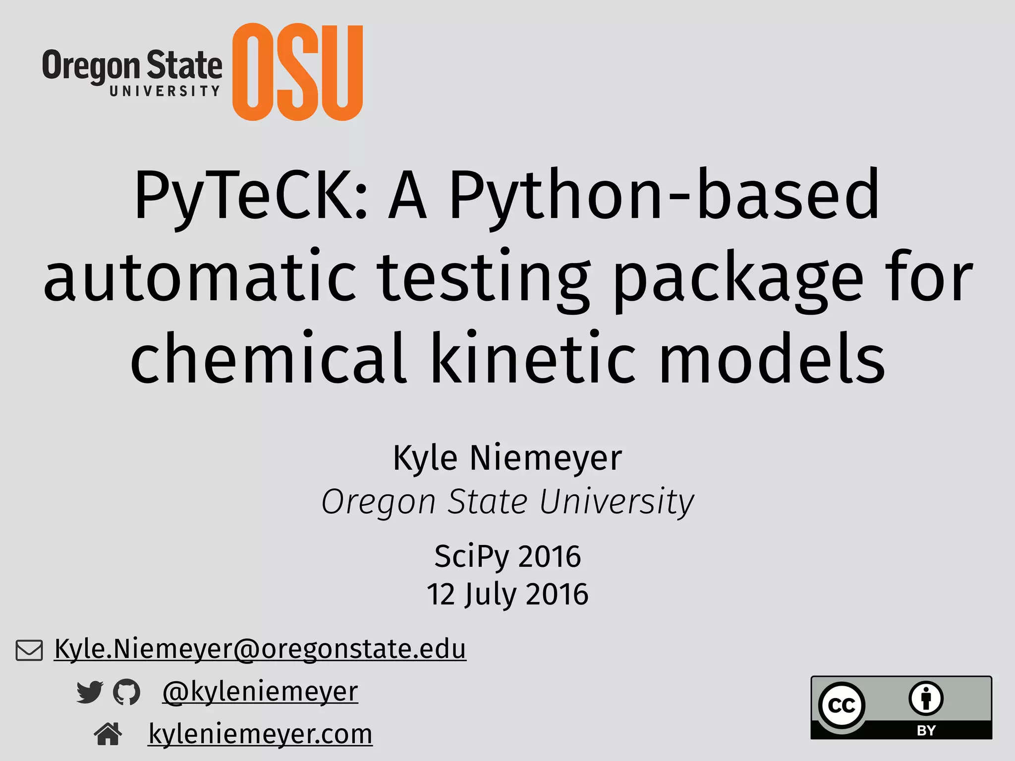
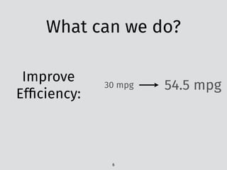
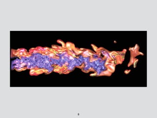
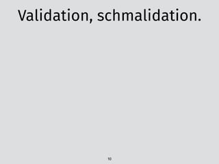
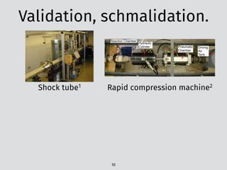
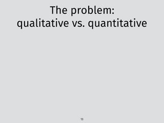
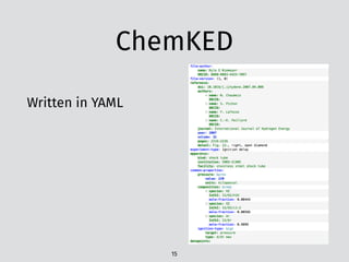
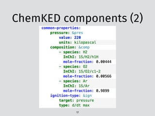
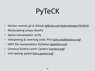
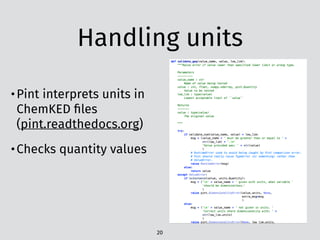
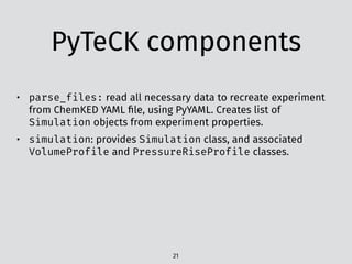
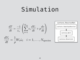
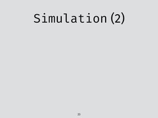
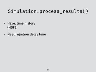
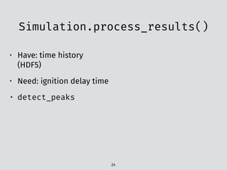
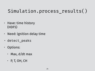
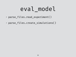
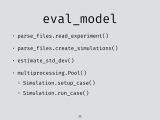
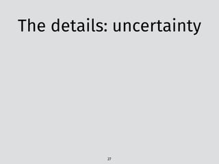
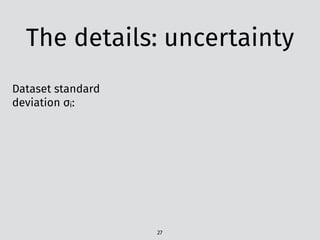
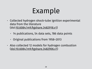
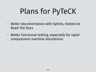
# n-heptane ignition delay from Colket and Spadaccini 2001
# P (atm), T (K), Ignition Delay (µs)
# Mole Fraction nC7H16 O2 Ar : 0.00192 0.04224 0.95584
7.72 ,1393 ,85
7.78 ,1299 ,345
7.04 ,1235 ,631
6.38 ,1299 ,348
7.53 ,1372 ,134
6.08 ,1236 ,678
7.35 ,1340 ,148
6.63 ,1328 ,211
6.94 ,1395 ,89
CSV file7](https://image.slidesharecdn.com/scipy2016-pyteck-160713162513/85/PyTeCK-A-Python-based-automatic-testing-package-for-chemical-kinetic-models-31-320.jpg)
![The problem:
experimental data
12
PDF table5
t [ms3 ~- metric benzene-air mixture.
region the dependence of the ignition delay
time upon temperature can be expressed ap-
proximately by straight lines in the Arrhenius
plot. The corresponding global activation ener-
gies decrease with increasing pressure.
For Ps around 13.5 bar the dependence be-
comes strongly nonlinear in a temperature
range between 950 and 700 K. In this interme-
diate temperature region a decrease in ignition
delay time is observed with decreasing temper-
atures. This leads to an S-shaped curve with a
maximum and a minimum. Between both ex-
termal values the dependence possesses a neg-
ative temperature coefficient. The position of
this transition region shifts to higher tempera-
tures with increasing pressures Ps- In the low-
temperature region--below approximately 700
K--the dependence of the ignition delay time
upon temperature can again be expressed by a
linear dependence. Because the measuring time
of the shock tube is limited, the delay times
could be determined only above 660 K, so that
only a short part of the low-temperature region
could be investigated in our experiments. The
influence of pressure on the ignition delay is
most pronounced in the transition region,
smallest for low temperatures and of varying
degree in the high-temperature region, where
with increasing temperature this dependence
becomes smaller.
"1~z
[ms]
101
100
1o-1
162
,, 3.2bar ,,./--~-~.~ /.-'~
o 6.s ,, ./ '---J.//
O I£3 " / ' / n [] ..~-/
30 ,,,, .o
,~_ D,,- x i< 3 bar 1 Comoufofion
~o/"°E~/" × ~+.---+-.---L_._.+_.~..~" ~ X13 " ,, [ , " ,
t/~ / /" !.ine of /+0 " j el'. a[.
/.z~ ~/ ./ pressure variation
,/~// T=9/,0 K (Fig.11) T
/ 1200 1000 800 [K]
I I I i I I I I I l I
0:8 1.o 1.2 114 loooK
T
Fig. 3. Ignition delay times.
Figure6
# n-heptane ignition delay from Colket and Spadaccini 2001
# P (atm), T (K), Ignition Delay (µs)
# Mole Fraction nC7H16 O2 Ar : 0.00192 0.04224 0.95584
7.72 ,1393 ,85
7.78 ,1299 ,345
7.04 ,1235 ,631
6.38 ,1299 ,348
7.53 ,1372 ,134
6.08 ,1236 ,678
7.35 ,1340 ,148
6.63 ,1328 ,211
6.94 ,1395 ,89
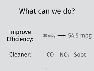
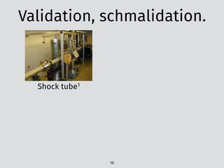
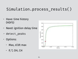
CSV file7 Email plea](https://image.slidesharecdn.com/scipy2016-pyteck-160713162513/85/PyTeCK-A-Python-based-automatic-testing-package-for-chemical-kinetic-models-32-320.jpg)
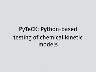
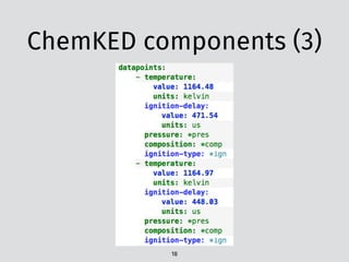
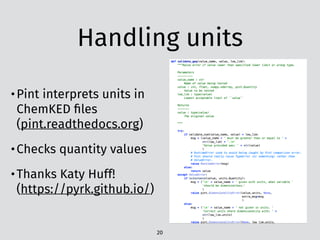
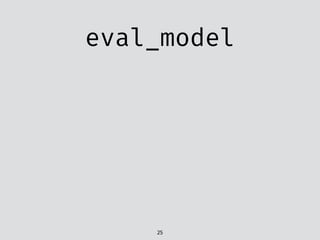
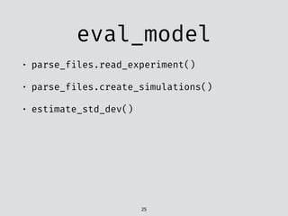
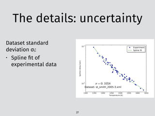
![The problem:
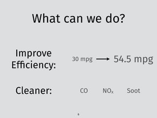
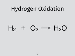
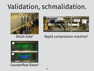
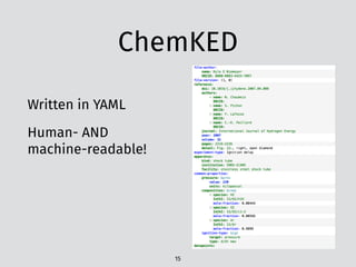
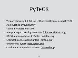
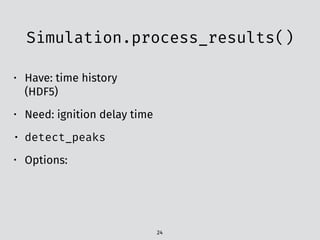
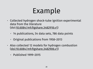
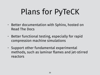
qualitative vs. quantitative
13
del
ne,
ne,
Re-
ng
ev-
he
an
ee-
ha-
ed
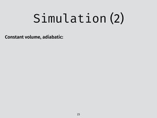
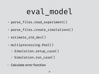
by sensitivity analysis [25–27], except for the small molecules
(i.e., C2H2, C2H3, CH2CO, HCCO, et al.) included in three-component
fuels mechanism [22]. Finally, a reduced sub-mechanism of tolu-
ene oxidation is formed and presented in Supplementary data A.
2.2. The sub-mechanism of DIB
A detailed mechanism considered two isomers of DIB, i.e. 2,4,
4-trimethyl-1-pentene (JC8H16) and 2,4,4-trimethyl-2-pentene
(IC8H16), was developed by Metcalfe et al. [28]. The detailed model
consists of 897 species and 3783 elementary reactions. However,
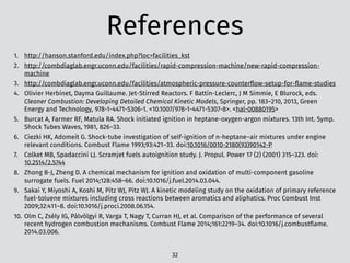
0.1
1
10
100
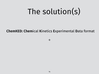
Toluene/N-heptane/air
Expt. Present
P = 5MPa
P = 3MPa
P = 1MPa
1000/T (1/K)
Ignitiondelaytime(ms)
(a) φ=1.0
0.8 0.9 1.0 1.1 1.2 1.3 1.4 1.5
1
10
100
Expt. Present
P = 5MPa
P = 3MPa
Toluene/N-heptane/air
Ignitiondelaytime(ms)](https://image.slidesharecdn.com/scipy2016-pyteck-160713162513/85/PyTeCK-A-Python-based-automatic-testing-package-for-chemical-kinetic-models-34-320.jpg)
![The problem:
qualitative vs. quantitative
13
del
ne,
ne,
Re-
ng
ev-
he
an
ee-
ha-
ed
by sensitivity analysis [25–27], except for the small molecules
(i.e., C2H2, C2H3, CH2CO, HCCO, et al.) included in three-component
fuels mechanism [22]. Finally, a reduced sub-mechanism of tolu-
ene oxidation is formed and presented in Supplementary data A.
2.2. The sub-mechanism of DIB
A detailed mechanism considered two isomers of DIB, i.e. 2,4,
4-trimethyl-1-pentene (JC8H16) and 2,4,4-trimethyl-2-pentene
(IC8H16), was developed by Metcalfe et al. [28]. The detailed model
consists of 897 species and 3783 elementary reactions. However,
0.1
1
10
100
Toluene/N-heptane/air
Expt. Present
P = 5MPa
P = 3MPa
P = 1MPa
1000/T (1/K)
Ignitiondelaytime(ms)
(a) φ=1.0
0.8 0.9 1.0 1.1 1.2 1.3 1.4 1.5
1
10
100
Expt. Present
P = 5MPa
P = 3MPa
Toluene/N-heptane/air
Ignitiondelaytime(ms)
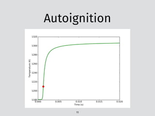
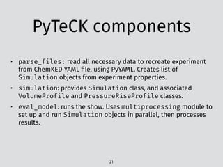
“…the calculations show
good agreements with
experiments…”8](https://image.slidesharecdn.com/scipy2016-pyteck-160713162513/85/PyTeCK-A-Python-based-automatic-testing-package-for-chemical-kinetic-models-35-320.jpg)
![The problem:
qualitative vs. quantitative
13
del
ne,
ne,
Re-
ng
ev-
he
an
ee-
ha-
ed
by sensitivity analysis [25–27], except for the small molecules
(i.e., C2H2, C2H3, CH2CO, HCCO, et al.) included in three-component
fuels mechanism [22]. Finally, a reduced sub-mechanism of tolu-
ene oxidation is formed and presented in Supplementary data A.
2.2. The sub-mechanism of DIB
A detailed mechanism considered two isomers of DIB, i.e. 2,4,
4-trimethyl-1-pentene (JC8H16) and 2,4,4-trimethyl-2-pentene
(IC8H16), was developed by Metcalfe et al. [28]. The detailed model
consists of 897 species and 3783 elementary reactions. However,
0.1
1
10
100
Toluene/N-heptane/air
Expt. Present
P = 5MPa
P = 3MPa
P = 1MPa
1000/T (1/K)
Ignitiondelaytime(ms)
(a) φ=1.0
0.8 0.9 1.0 1.1 1.2 1.3 1.4 1.5
1
10
100
Expt. Present
P = 5MPa
P = 3MPa
Toluene/N-heptane/air
Ignitiondelaytime(ms)
“…the calculations show
good agreements with
experiments…”8
“…although there is a
mismatch […] at […] T < 1000 K.”](https://image.slidesharecdn.com/scipy2016-pyteck-160713162513/85/PyTeCK-A-Python-based-automatic-testing-package-for-chemical-kinetic-models-36-320.jpg)
![The problem:
qualitative vs. quantitative
13
del
ne,
ne,
Re-
ng
ev-
he
an
ee-
ha-
ed
by sensitivity analysis [25–27], except for the small molecules
(i.e., C2H2, C2H3, CH2CO, HCCO, et al.) included in three-component
fuels mechanism [22]. Finally, a reduced sub-mechanism of tolu-
ene oxidation is formed and presented in Supplementary data A.
2.2. The sub-mechanism of DIB
A detailed mechanism considered two isomers of DIB, i.e. 2,4,
4-trimethyl-1-pentene (JC8H16) and 2,4,4-trimethyl-2-pentene
(IC8H16), was developed by Metcalfe et al. [28]. The detailed model
consists of 897 species and 3783 elementary reactions. However,
0.1
1
10
100
Toluene/N-heptane/air
Expt. Present
P = 5MPa
P = 3MPa
P = 1MPa
1000/T (1/K)
Ignitiondelaytime(ms)
(a) φ=1.0
0.8 0.9 1.0 1.1 1.2 1.3 1.4 1.5
1
10
100
Expt. Present
P = 5MPa
P = 3MPa
Toluene/N-heptane/air
Ignitiondelaytime(ms)
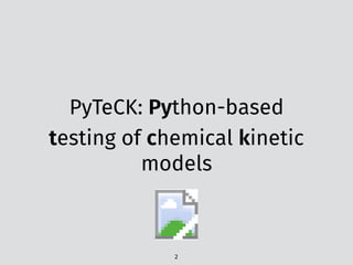
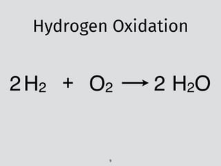
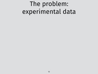
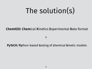
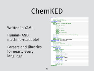
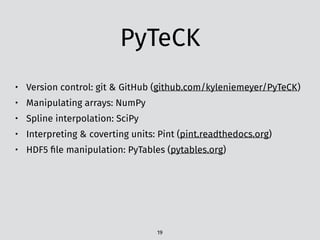
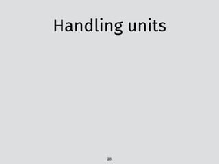
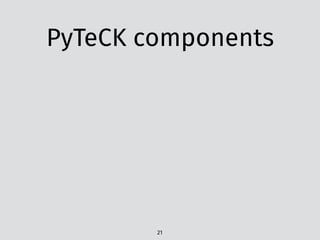
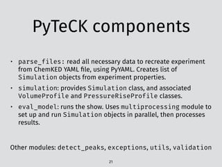
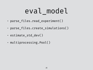
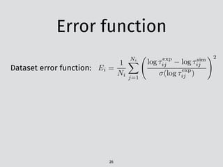
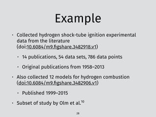
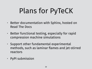
model. Figure 5 shows the comparison of the igni-
tion delay times of PRF/toluene mixtures at 25
and 50 atm [1]. The species mole fractions in the
oxidation of PRF/toluene at 12.5 atm obtained
by a flow reactor experiment [7] are compared in
Fig. 6. Those figures indicate that the present
model well predicts the reactivity of PRF/toluene
mixtures at wide range of temperature and pres-
(dashed
addition
reproduc
mixtures
of cross
Reac
perform
PRF/tol
10
0.6 0.7 0.8 0.9
T-1
(103
K-1
)
12 atm
50 atm
Fig. 2. Comparisons of measured and simulated ignition
delay times of toluene at the equivalence ratio of 0.5%
and 1.2% fuels diluted in Ar or air behind reflected shock
waves at 2 [33], 15 and 50 atm [34]. Solid curves: present
model, dashed curves: Pitz model.
10
100
1000
10000
0.75 0.80 0.85 0.90 0.95 1.00
T-1
(103
K-1
)
Ignitiondelaytimes(µs)
Fig. 3. Comparisons of measured and simulated ignition
delay times of toluene behind reflected shock waves at
50 atm [34]. Solid curves: present model, dashed curves:
Pitz model.
0.00
Fig. 4.
CO + CO
by the flo
of initial
dashed cu
1
10
70
Ignitiondelaytimes(µs)
Fig. 5. C
delay tim
heptane/i
shock wa
present m
“…the calculations show
good agreements with
experiments…”8
“…although there is a
mismatch […] at […] T < 1000 K.”](https://image.slidesharecdn.com/scipy2016-pyteck-160713162513/85/PyTeCK-A-Python-based-automatic-testing-package-for-chemical-kinetic-models-37-320.jpg)
![The problem:
qualitative vs. quantitative
13
del
ne,
ne,
Re-
ng
ev-
he
an
ee-
ha-
ed
by sensitivity analysis [25–27], except for the small molecules
(i.e., C2H2, C2H3, CH2CO, HCCO, et al.) included in three-component
fuels mechanism [22]. Finally, a reduced sub-mechanism of tolu-
ene oxidation is formed and presented in Supplementary data A.
2.2. The sub-mechanism of DIB
A detailed mechanism considered two isomers of DIB, i.e. 2,4,
4-trimethyl-1-pentene (JC8H16) and 2,4,4-trimethyl-2-pentene
(IC8H16), was developed by Metcalfe et al. [28]. The detailed model
consists of 897 species and 3783 elementary reactions. However,
0.1
1
10
100
Toluene/N-heptane/air
Expt. Present
P = 5MPa
P = 3MPa
P = 1MPa
1000/T (1/K)
Ignitiondelaytime(ms)
(a) φ=1.0
0.8 0.9 1.0 1.1 1.2 1.3 1.4 1.5
1
10
100
Expt. Present
P = 5MPa
P = 3MPa
Toluene/N-heptane/air
Ignitiondelaytime(ms)
model. Figure 5 shows the comparison of the igni-
tion delay times of PRF/toluene mixtures at 25
and 50 atm [1]. The species mole fractions in the
oxidation of PRF/toluene at 12.5 atm obtained
by a flow reactor experiment [7] are compared in
Fig. 6. Those figures indicate that the present
model well predicts the reactivity of PRF/toluene
mixtures at wide range of temperature and pres-
(dashed
addition
reproduc
mixtures
of cross
Reac
perform
PRF/tol
10
0.6 0.7 0.8 0.9
T-1
(103
K-1
)
12 atm
50 atm
Fig. 2. Comparisons of measured and simulated ignition
delay times of toluene at the equivalence ratio of 0.5%
and 1.2% fuels diluted in Ar or air behind reflected shock
waves at 2 [33], 15 and 50 atm [34]. Solid curves: present
model, dashed curves: Pitz model.
10
100
1000
10000
0.75 0.80 0.85 0.90 0.95 1.00
T-1
(103
K-1
)
Ignitiondelaytimes(µs)
Fig. 3. Comparisons of measured and simulated ignition
delay times of toluene behind reflected shock waves at
50 atm [34]. Solid curves: present model, dashed curves:
Pitz model.
0.00
Fig. 4.
CO + CO
by the flo
of initial
dashed cu
1
10
70
Ignitiondelaytimes(µs)
Fig. 5. C
delay tim
heptane/i
shock wa
present m
“In general, the present
model predicts well the
reactivity of […] mixtures…”9
“…the calculations show
good agreements with
experiments…”8
“…although there is a
mismatch […] at […] T < 1000 K.”](https://image.slidesharecdn.com/scipy2016-pyteck-160713162513/85/PyTeCK-A-Python-based-automatic-testing-package-for-chemical-kinetic-models-38-320.jpg)


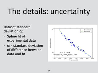
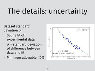


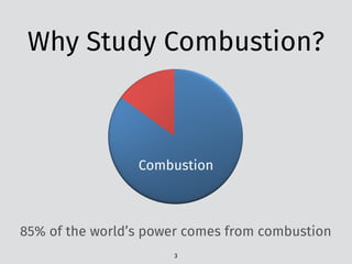
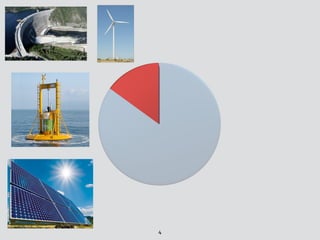
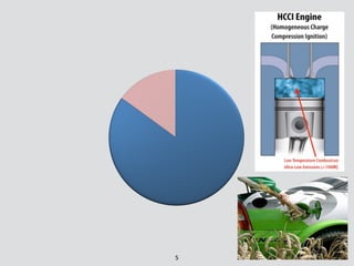
The document discusses PyTeck, a Python-based testing package designed for chemical kinetic models, emphasizing its relevance to combustion research, which accounts for 85% of the world's power. It covers various topics including the construction and validation of jet-stirred reactors and the complexities of ignition delay times in different fuel-air mixtures under varying pressures and temperatures. Additionally, it explores qualitative versus quantitative challenges in combustion modeling and presents mechanisms relating to fuels like toluene and n-heptane.


![[W f stoecker]_refrigeration_and_a_ir_conditioning_(book_zz.org)](https://cdn.slidesharecdn.com/ss_thumbnails/wfstoeckerrefrigerationandairconditioningbookzz-161019162540-thumbnail.jpg?width=640&height=640&fit=bounds)


