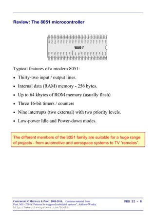
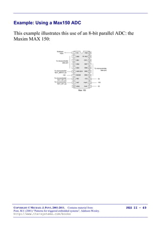
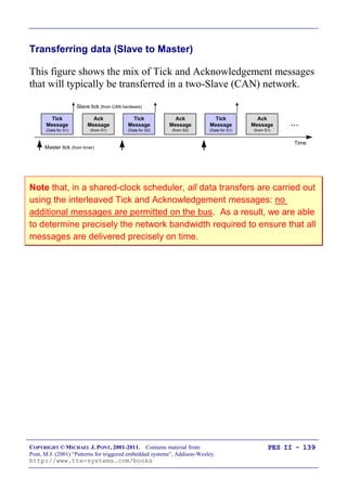
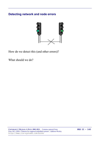
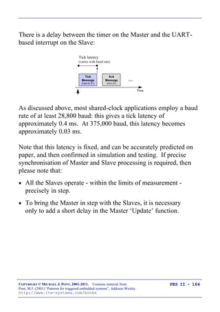
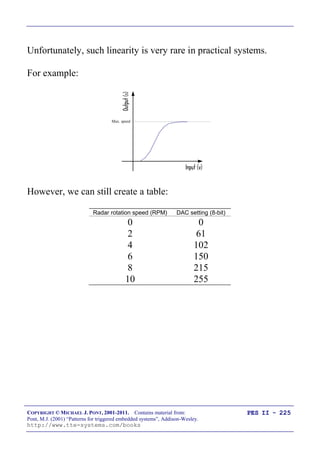
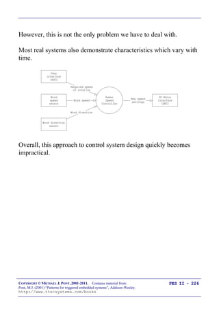
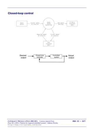
This document provides an overview of a 10-week course on embedded systems using C programming. It discusses the design and implementation of a flexible scheduler for single-processor embedded systems over the course of two seminar sessions. The scheduler will allow tasks to be added and deleted dynamically. The document outlines the key topics that will be covered in each seminar, including an introduction to schedulers, building a basic scheduler, analog I/O, PID control, and linking multiple processors together using various communication protocols.
![I
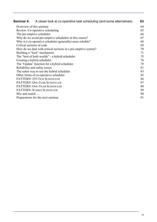
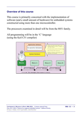
Programming
Embedded
Systems II
A 10-week course, using C
40
39
38
37
36
35
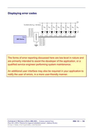
34
1
2
3
4
5
6
7
„8051‟
8
9
10
33
32
31
30
29
28
27
26
25
24
11
12
13
14
15
16
17
18
19
20
23
22
21
P3.0
P1.7
RST
P1.6
P1.5
P1.4
P1.2
P1.3
P1.1
P1.0
VSS
XTL2
XTL1
P3.7
P3.6
P3.5
P3.3
P3.4
P3.2
P3.1
/EA
P0.6
P0.7
P0.5
P0.4
P0.3
P0.1
P0.2
P0.0
VCC
P2.0
P2.2
P2.1
P2.3
P2.4
P2.5
P2.7
P2.6
/PSEN
ALE
Michael J. Pont
University of Leicester
[v2.3]
Further info:
http://www.tte-systems.com/services/Certified_Embedded_C_Programmer](https://image.slidesharecdn.com/programmingembeddedsystemsii-200229112938/85/Programming-embedded-systems-ii-1-320.jpg)


![IX
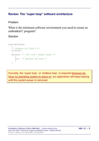
Seminar 7: Linking processors using RS-232 and RS-485 protocols 153
Review: Shared-clock scheduling 154
Overview of this seminar 155
Review: What is „RS-232‟? 156
Review: Basic RS-232 Protocol 157
Review: Transferring data to a PC using RS-232 158
PATTERN: SCU SCHEDULER (LOCAL) 159
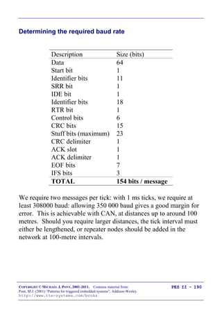
The message structure 160
Determining the required baud rate 163
Node Hardware 165
Network wiring 166
Overall strengths and weaknesses 167
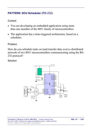
PATTERN: SCU Scheduler (RS-232) 168
PATTERN: SCU Scheduler (RS-485) 169
RS-232 vs RS-485 [number of nodes] 170
RS-232 vs RS-485 [range and baud rates] 171
RS-232 vs RS-485 [cabling] 172
RS-232 vs RS-485 [transceivers] 173
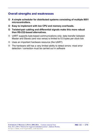
Software considerations: enable inputs 174
Overall strengths and weaknesses 175
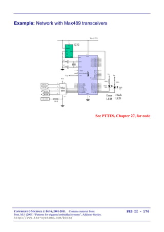
Example: Network with Max489 transceivers 176
Preparations for the next seminar 177](https://image.slidesharecdn.com/programmingembeddedsystemsii-200229112938/85/Programming-embedded-systems-ii-9-320.jpg)

![COPYRIGHT © MICHAEL J. PONT, 2001-2011. Contains material from:
Pont, M.J. (2001) “Patterns for triggered embedded systems”, Addison-Wesley.
http://www.tte-systems.com/books
PES II - 5
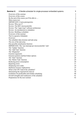
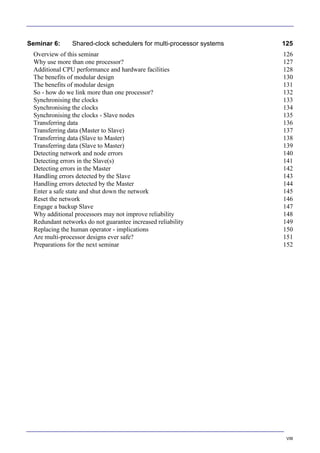
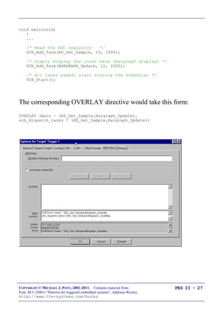
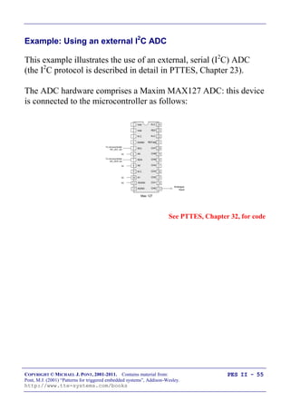
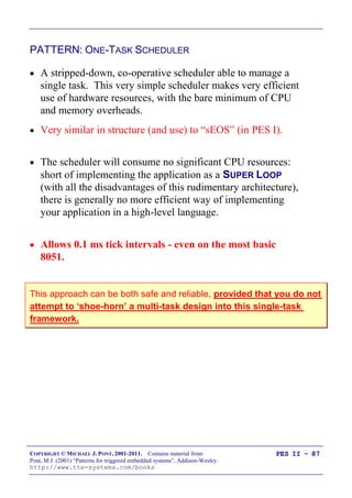
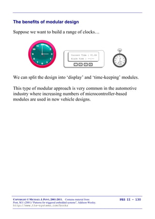
Main course text
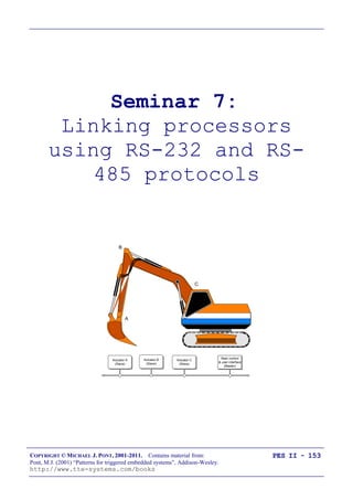
Throughout this course, we will be making heavy use of this book:
Patterns for time-triggered embedded
systems: Building reliable applications with
the 8051 family of microcontrollers,
by Michael J. Pont (2001)
Addison-Wesley / ACM Press.
[ISBN: 0-201-331381]
You can download this book (PDF) here:
http://www.tte-systems.com/books/pttes](https://image.slidesharecdn.com/programmingembeddedsystemsii-200229112938/85/Programming-embedded-systems-ii-18-320.jpg)
![COPYRIGHT © MICHAEL J. PONT, 2001-2011. Contains material from:
Pont, M.J. (2001) “Patterns for triggered embedded systems”, Addison-Wesley.
http://www.tte-systems.com/books
PES II - 15
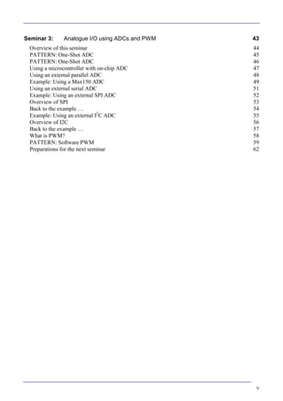
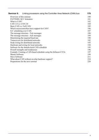
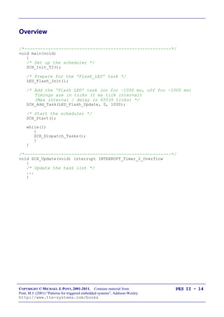
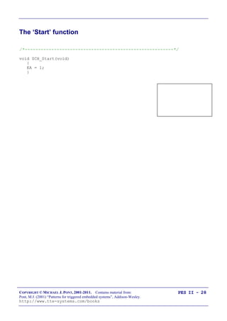
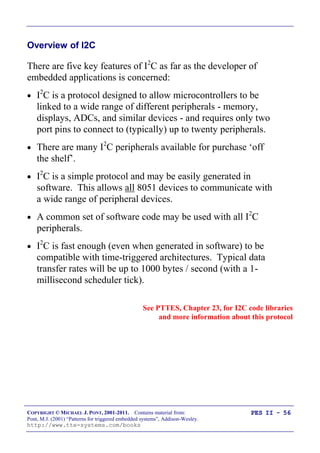
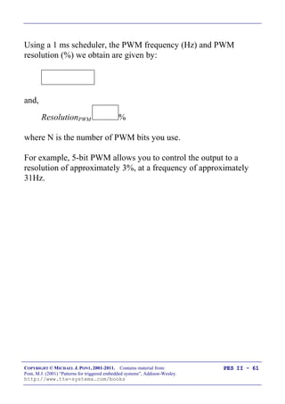
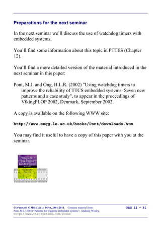
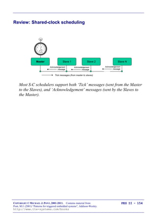
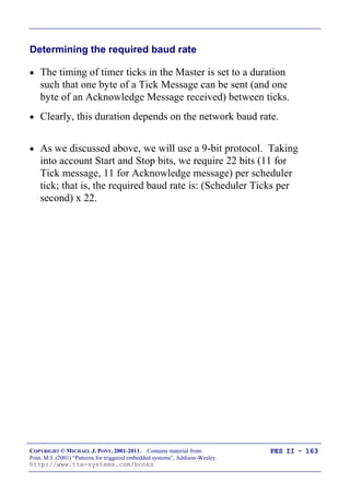
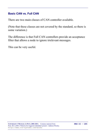
The scheduler data structure and task array
/* Store in DATA area, if possible, for rapid access
Total memory per task is 7 bytes */
typedef data struct
{
/* Pointer to the task (must be a 'void (void)' function) */
void (code * pTask)(void);
/* Delay (ticks) until the function will (next) be run
- see SCH_Add_Task() for further details */
tWord Delay;
/* Interval (ticks) between subsequent runs.
- see SCH_Add_Task() for further details */
tWord Repeat;
/* Incremented (by scheduler) when task is due to execute */
tByte RunMe;
} sTask;
File Sch51.H also includes the constant SCH_MAX_TASKS:
/* The maximum number of tasks required at any one time
during the execution of the program
MUST BE ADJUSTED FOR EACH NEW PROJECT */
#define SCH_MAX_TASKS (1)
Both the sTask data type and the SCH_MAX_TASKS constant are
used to create - in the file Sch51.C - the array of tasks that is
referred to throughout the scheduler:
/* The array of tasks */
sTask SCH_tasks_G[SCH_MAX_TASKS];](https://image.slidesharecdn.com/programmingembeddedsystemsii-200229112938/85/Programming-embedded-systems-ii-28-320.jpg)
![COPYRIGHT © MICHAEL J. PONT, 2001-2011. Contains material from:
Pont, M.J. (2001) “Patterns for triggered embedded systems”, Addison-Wesley.
http://www.tte-systems.com/books
PES II - 19
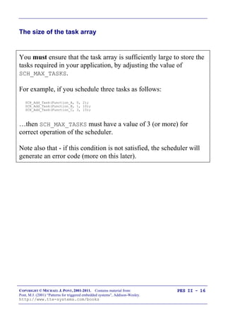
The „Update‟ function
/*--------------------------------------------------------*/
void SCH_Update(void) interrupt INTERRUPT_Timer_2_Overflow
{
tByte Index;
TF2 = 0; /* Have to manually clear this. */
/* NOTE: calculations are in *TICKS* (not milliseconds) */
for (Index = 0; Index < SCH_MAX_TASKS; Index++)
{
/* Check if there is a task at this location */
if (SCH_tasks_G[Index].pTask)
{
if (--SCH_tasks_G[Index].Delay == 0)
{
/* The task is due to run */
SCH_tasks_G[Index].RunMe += 1; /* Inc. 'RunMe' flag */
if (SCH_tasks_G[Index].Period)
{
/* Schedule regular tasks to run again */
SCH_tasks_G[Index].Delay = SCH_tasks_G[Index].Period;
}
}
}
}
}](https://image.slidesharecdn.com/programmingembeddedsystemsii-200229112938/85/Programming-embedded-systems-ii-32-320.jpg)
![COPYRIGHT © MICHAEL J. PONT, 2001-2011. Contains material from:
Pont, M.J. (2001) “Patterns for triggered embedded systems”, Addison-Wesley.
http://www.tte-systems.com/books
PES II - 21
/*--------------------------------------------------------*-
SCH_Add_Task()
Causes a task (function) to be executed at regular
intervals, or after a user-defined delay.
-*--------------------------------------------------------*/
tByte SCH_Add_Task(void (code * pFunction)(),
const tWord DELAY,
const tWord PERIOD)
{
tByte Index = 0;
/* First find a gap in the array (if there is one) */
while ((SCH_tasks_G[Index].pTask != 0) && (Index < SCH_MAX_TASKS))
{
Index++;
}
/* Have we reached the end of the list? */
if (Index == SCH_MAX_TASKS)
{
/* Task list is full
-> set the global error variable */
Error_code_G = ERROR_SCH_TOO_MANY_TASKS;
/* Also return an error code */
return SCH_MAX_TASKS;
}
/* If we're here, there is a space in the task array */
SCH_tasks_G[Index].pTask = pFunction;
SCH_tasks_G[Index].Delay = DELAY + 1;
SCH_tasks_G[Index].Period = PERIOD;
SCH_tasks_G[Index].RunMe = 0;
return Index; /* return pos. of task (to allow deletion) */
}](https://image.slidesharecdn.com/programmingembeddedsystemsii-200229112938/85/Programming-embedded-systems-ii-34-320.jpg)
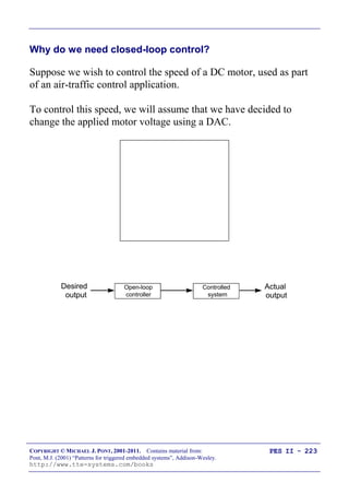
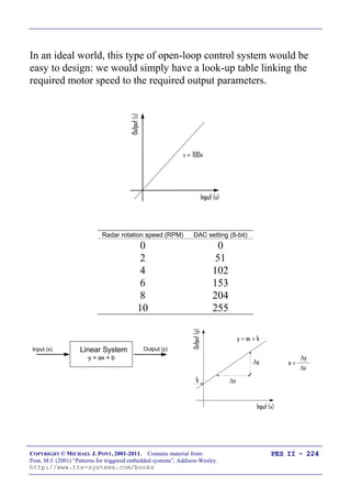
![COPYRIGHT © MICHAEL J. PONT, 2001-2011. Contains material from:
Pont, M.J. (2001) “Patterns for triggered embedded systems”, Addison-Wesley.
http://www.tte-systems.com/books
PES II - 22
The „Dispatcher‟
/*--------------------------------------------------------*-
SCH_Dispatch_Tasks()
This is the 'dispatcher' function. When a task (function)
is due to run, SCH_Dispatch_Tasks() will run it.
This function must be called (repeatedly) from the main loop.
-*--------------------------------------------------------*/
void SCH_Dispatch_Tasks(void)
{
tByte Index;
/* Dispatches (runs) the next task (if one is ready) */
for (Index = 0; Index < SCH_MAX_TASKS; Index++)
{
if (SCH_tasks_G[Index].RunMe > 0)
{
(*SCH_tasks_G[Index].pTask)(); /* Run the task */
SCH_tasks_G[Index].RunMe -= 1; /* Reduce RunMe count */
/* Periodic tasks will automatically run again
- if this is a 'one shot' task, delete it */
if (SCH_tasks_G[Index].Period == 0)
{
SCH_Delete_Task(Index);
}
}
}
/* Report system status */
SCH_Report_Status();
/* The scheduler enters idle mode at this point */
SCH_Go_To_Sleep();
}](https://image.slidesharecdn.com/programmingembeddedsystemsii-200229112938/85/Programming-embedded-systems-ii-35-320.jpg)
![COPYRIGHT © MICHAEL J. PONT, 2001-2011. Contains material from:
Pont, M.J. (2001) “Patterns for triggered embedded systems”, Addison-Wesley.
http://www.tte-systems.com/books
PES II - 25
Function pointers and Keil linker options
When we write:
SCH_Add_Task(Do_X,1000,0);
…the first parameter of the „Add Task‟ function is a pointer to the
function Do_X().
This function pointer is then passed to the Dispatch function and it
is through this function that the task is executed:
if (SCH_tasks_G[Index].RunMe > 0)
{
(*SCH_tasks_G[Index].pTask)(); /* Run the task */
BUT
The linker has difficulty determining the correct call tree when function
pointers are used as arguments.](https://image.slidesharecdn.com/programmingembeddedsystemsii-200229112938/85/Programming-embedded-systems-ii-38-320.jpg)
![COPYRIGHT © MICHAEL J. PONT, 2001-2011. Contains material from:
Pont, M.J. (2001) “Patterns for triggered embedded systems”, Addison-Wesley.
http://www.tte-systems.com/books
PES II - 29
The „Delete Task‟ function
When tasks are added to the task array, SCH_Add_Task() returns
the position in the task array at which the task has been added:
Task_ID = SCH_Add_Task(Do_X,1000,0);
Sometimes it can be necessary to delete tasks from the array.
You can do so as follows: SCH_Delete_Task(Task_ID);
bit SCH_Delete_Task(const tByte TASK_INDEX)
{
bit Return_code;
if (SCH_tasks_G[TASK_INDEX].pTask == 0)
{
/* No task at this location...
-> set the global error variable */
Error_code_G = ERROR_SCH_CANNOT_DELETE_TASK;
/* ...also return an error code */
Return_code = RETURN_ERROR;
}
else
{
Return_code = RETURN_NORMAL;
}
SCH_tasks_G[TASK_INDEX].pTask = 0x0000;
SCH_tasks_G[TASK_INDEX].Delay = 0;
SCH_tasks_G[TASK_INDEX].Period = 0;
SCH_tasks_G[TASK_INDEX].RunMe = 0;
return Return_code; /* return status */
}](https://image.slidesharecdn.com/programmingembeddedsystemsii-200229112938/85/Programming-embedded-systems-ii-42-320.jpg)


![COPYRIGHT © MICHAEL J. PONT, 2001-2011. Contains material from:
Pont, M.J. (2001) “Patterns for triggered embedded systems”, Addison-Wesley.
http://www.tte-systems.com/books
PES II - 67
Why do we avoid pre-emptive schedulers in this course?
Various research studies have demonstrated that, compared to pre-
emptive schedulers, co-operative schedulers have a number of
desirable features, particularly for use in safety-related systems.
“[Pre-emptive] schedules carry greater runtime overheads
because of the need for context switching - storage and retrieval
of partially computed results. [Co-operative] algorithms do not
incur such overheads. Other advantages of [co-operative]
algorithms include their better understandability, greater
predictability, ease of testing and their inherent capability for
guaranteeing exclusive access to any shared resource or data.”.
Nissanke (1997, p.237)
“Significant advantages are obtained when using this [co-
operative] technique. Since the processes are not interruptable,
poor synchronisation does not give rise to the problem of
shared data. Shared subroutines can be implemented without
producing re-entrant code or implementing lock and unlock
mechanisms”.
Allworth (1981, p.53-54)
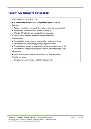
Compared to pre-emptive alternatives, co-operative schedulers
have the following advantages: [1] The scheduler is simpler; [2]
The overheads are reduced; [3] Testing is easier; [4]
Certification authorities tend to support this form of scheduling.
Bate (2000)
[See PTTES, Chapter 13]](https://image.slidesharecdn.com/programmingembeddedsystemsii-200229112938/85/Programming-embedded-systems-ii-80-320.jpg)
![COPYRIGHT © MICHAEL J. PONT, 2001-2011. Contains material from:
Pont, M.J. (2001) “Patterns for triggered embedded systems”, Addison-Wesley.
http://www.tte-systems.com/books
PES II - 76
Creating a hybrid scheduler
The „update‟ function from a co-operative scheduler:
void SCH_Update(void) interrupt INTERRUPT_Timer_2_Overflow
{
tByte Index;
TF2 = 0; /* Have to manually clear this. */
/* NOTE: calculations are in *TICKS* (not milliseconds) */
for (Index = 0; Index < SCH_MAX_TASKS; Index++)
{
/* Check if there is a task at this location */
if (SCH_tasks_G[Index].Task_p)
{
if (--SCH_tasks_G[Index].Delay == 0)
{
/* The task is due to run */
SCH_tasks_G[Index].RunMe += 1; /* Inc. RunMe */
if (SCH_tasks_G[Index].Period)
{
/* Schedule periodic tasks to run again */
SCH_tasks_G[Index].Delay = SCH_tasks_G[Index].Period;
}
}
}
}
}](https://image.slidesharecdn.com/programmingembeddedsystemsii-200229112938/85/Programming-embedded-systems-ii-89-320.jpg)
![COPYRIGHT © MICHAEL J. PONT, 2001-2011. Contains material from:
Pont, M.J. (2001) “Patterns for triggered embedded systems”, Addison-Wesley.
http://www.tte-systems.com/books
PES II - 77
The co-operative version assumes a scheduler data type as follows:
/* Store in DATA area, if possible, for rapid access
[Total memory per task is 7 bytes] */
typedef data struct
{
/* Pointer to the task (must be a 'void (void)' function) */
void (code * Task_p)(void);
/* Delay (ticks) until the function will (next) be run
- see SCH_Add_Task() for further details */
tWord Delay;
/* Interval (ticks) between subsequent runs.
- see SCH_Add_Task() for further details */
tWord Period;
/* Set to 1 (by scheduler) when task is due to execute */
tByte RunMe;
} sTask;](https://image.slidesharecdn.com/programmingembeddedsystemsii-200229112938/85/Programming-embedded-systems-ii-90-320.jpg)
![COPYRIGHT © MICHAEL J. PONT, 2001-2011. Contains material from:
Pont, M.J. (2001) “Patterns for triggered embedded systems”, Addison-Wesley.
http://www.tte-systems.com/books
PES II - 78
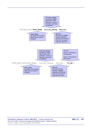
The „Update‟ function for a hybrid scheduler.
void hSCH_Update(void) interrupt INTERRUPT_Timer_2_Overflow
{
tByte Index;
TF2 = 0; /* Have to manually clear this. */
/* NOTE: calculations are in *TICKS* (not milliseconds) */
for (Index = 0; Index < hSCH_MAX_TASKS; Index++)
{
/* Check if there is a task at this location */
if (hSCH_tasks_G[Index].pTask)
{
if (--hSCH_tasks_G[Index].Delay == 0)
{
/* The task is due to run */
if (hSCH_tasks_G[Index].Co_op)
{
/* If it is co-op, inc. RunMe */
hSCH_tasks_G[Index].RunMe += 1;
}
else
{
/* If it is a pre-emp, run it IMMEDIATELY */
(*hSCH_tasks_G[Index].pTask)();
hSCH_tasks_G[Index].RunMe -= 1; /* Dec RunMe */
/* Periodic tasks will automatically run again
- if this is a 'one shot' task, delete it. */
if (hSCH_tasks_G[Index].Period == 0)
{
hSCH_tasks_G[Index].pTask = 0;
}
}
if (hSCH_tasks_G[Index].Period)
{
/* Schedule regular tasks to run again */
hSCH_tasks_G[Index].Delay = hSCH_tasks_G[Index].Period;
}
}
}
}](https://image.slidesharecdn.com/programmingembeddedsystemsii-200229112938/85/Programming-embedded-systems-ii-91-320.jpg)
![COPYRIGHT © MICHAEL J. PONT, 2001-2011. Contains material from:
Pont, M.J. (2001) “Patterns for triggered embedded systems”, Addison-Wesley.
http://www.tte-systems.com/books
PES II - 79
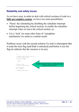
The hybrid version assumes a scheduler data type as follows:
/* Store in DATA area, if possible, for rapid access
[Total memory per task is 8 bytes] */
typedef data struct
{
/* Pointer to the task (must be a 'void (void)' function) */
void (code * Task_p)(void);
/* Delay (ticks) until the function will (next) be run
- see SCH_Add_Task() for further details. */
tWord Delay;
/* Interval (ticks) between subsequent runs.
- see SCH_Add_Task() for further details. */
tWord Period;
/* Set to 1 (by scheduler) when task is due to execute */
tByte RunMe;
/* Set to 1 if task is co-operative;
Set to 0 if task is pre-emptive. */
tByte Co_op;
} sTask;](https://image.slidesharecdn.com/programmingembeddedsystemsii-200229112938/85/Programming-embedded-systems-ii-92-320.jpg)
![COPYRIGHT © MICHAEL J. PONT, 2001-2011. Contains material from:
Pont, M.J. (2001) “Patterns for triggered embedded systems”, Addison-Wesley.
http://www.tte-systems.com/books
PES II - 85
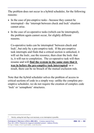
Other forms of co-operative scheduler
255-TICK SCHEDULER [PTTES, p.747]
A scheduler designed to run multiple tasks, but with reduced
memory (and CPU) overheads. This scheduler operates in
the same way as the standard co-operative schedulers, but
all information is stored in byte-sized (rather than word-
sized) variables: this reduces the required memory for each
task by around 30%.
ONE-TASK SCHEDULER [PTTES, p.749]
A stripped-down, co-operative scheduler able to manage a
single task. This very simple scheduler makes very efficient
use of hardware resources, with the bare minimum of CPU
and memory overheads.
ONE-YEAR SCHEDULER [PTTES, p.755]
A scheduler designed for very low-power operation:
specifically, it is designed to form the basis of battery-
powered applications capable of operating for a year or
more from a small, low-cost, battery supply.
STABLE SCHEDULER [PTTES, p.932]
is a temperature-compensated scheduler that adjusts its
behaviour to take into account changes in ambient
temperature.](https://image.slidesharecdn.com/programmingembeddedsystemsii-200229112938/85/Programming-embedded-systems-ii-98-320.jpg)
![COPYRIGHT © MICHAEL J. PONT, 2001-2011. Contains material from:
Pont, M.J. (2001) “Patterns for triggered embedded systems”, Addison-Wesley.
http://www.tte-systems.com/books
PES II - 86
PATTERN: 255-TICK SCHEDULER
A scheduler designed to run multiple tasks, but with reduced
memory (and CPU) overheads. This scheduler operates in
the same way as the standard co-operative schedulers, but
all information is stored in byte-sized (rather than word-
sized) variables: this reduces the required memory for each
task by around 30%.
/* Store in DATA area, if possible, for rapid access
[Total memory per task is 5 bytes)] */
typedef data struct
{
/* Pointer to the task (must be a 'void (void)' function) */
void (code * pTask)(void);
/* Delay (ticks) until the function will (next) be run
- see SCH_Add_Task() for further details. */
tByte Delay;
/* Interval (ticks) between subsequent runs.
- see SCH_Add_Task() for further details. */
tByte Period;
/* Incremented (by scheduler) when task is due to execute */
tByte RunMe;
} sTask;](https://image.slidesharecdn.com/programmingembeddedsystemsii-200229112938/85/Programming-embedded-systems-ii-99-320.jpg)

![COPYRIGHT © MICHAEL J. PONT, 2001-2011. Contains material from:
Pont, M.J. (2001) “Patterns for triggered embedded systems”, Addison-Wesley.
http://www.tte-systems.com/books
PES II - 89
PATTERN: STABLE SCHEDULER
A temperature-compensated scheduler that adjusts its
behaviour to take into account changes in ambient
temperature.
/* The temperature compensation data
The Timer 2 reload values (low and high bytes) are varied depending
on the current average temperature.
NOTE (1):
Only temperature values from 10 - 30 celsius are considered
in this version
NOTE (2):
Adjust these values to match your hardware! */
tByte code T2_reload_L[21] =
/* 10 11 12 13 14 15 16 17 18 19 */
{0xBA,0xB9,0xB8,0xB7,0xB6,0xB5,0xB4,0xB3,0xB2,0xB1,
/* 20 21 22 23 24 25 26 27 28 29 30 */
0xB0,0xAF,0xAE,0xAD,0xAC,0xAB,0xAA,0xA9,0xA8,0xA7,0xA6};
tByte code T2_reload_H[21] =
/* 10 11 12 13 14 15 16 17 18 19 */
{0x3C,0x3C,0x3C,0x3C,0x3C,0x3C,0x3C,0x3C,0x3C,0x3C,
/* 20 21 22 23 24 25 26 27 28 29 30 */
0x3C,0x3C,0x3C,0x3C,0x3C,0x3C,0x3C,0x3C,0x3C,0x3C,0x3C};](https://image.slidesharecdn.com/programmingembeddedsystemsii-200229112938/85/Programming-embedded-systems-ii-102-320.jpg)
![COPYRIGHT © MICHAEL J. PONT, 2001-2011. Contains material from:
Pont, M.J. (2001) “Patterns for triggered embedded systems”, Addison-Wesley.
http://www.tte-systems.com/books
PES II - 90
Mix and match …
Many of these different techniques can be combined
For example, using the one-year and one-task schedulers
together will further reduce current consumption.
For example, using the “stable scheduler” as the Master
node in a multi-processor system will improve the time-
keeping in the whole network
[More on this in later seminars …]](https://image.slidesharecdn.com/programmingembeddedsystemsii-200229112938/85/Programming-embedded-systems-ii-103-320.jpg)

![COPYRIGHT © MICHAEL J. PONT, 2001-2011. Contains material from:
Pont, M.J. (2001) “Patterns for triggered embedded systems”, Addison-Wesley.
http://www.tte-systems.com/books
PES II - 98
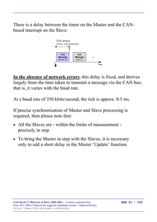
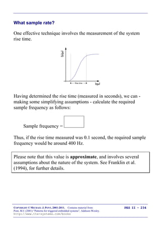
Time-based error detection
A key requirement in applications using a co-operative scheduler is
that, for all tasks, under all circumstances, the following condition
must be adhered to:
Where: is the task duration, and is the system
„tick interval‟.
It is possible to use a watchdog timer to detect task overflows, as
follows:
Set the watchdog timer to overflow at a period greater than
the tick interval.
Create a task that will update the watchdog timer shortly
before it overflows.
Start the watchdog.
[We‟ll say more about this shortly]](https://image.slidesharecdn.com/programmingembeddedsystemsii-200229112938/85/Programming-embedded-systems-ii-111-320.jpg)
![COPYRIGHT © MICHAEL J. PONT, 2001-2011. Contains material from:
Pont, M.J. (2001) “Patterns for triggered embedded systems”, Addison-Wesley.
http://www.tte-systems.com/books
PES II - 110
Dealing with errors
Here, we will assume that the PCEH will consist mainly of a loop:
/* Force watchdog timeout */
while(1)
;
This means that, as discussed in WATCHDOG RECOVERY [this
seminar] the watchdog timer will force a clean system reset.
Please note that, as also discussed in WATCHDOG RECOVERY, we
may be able to reduce the time taken to reset the processor by
adapting the watchdog timing. For example:
/* Set up the watchdog for “normal” use
- overflow period = ~39 ms */
WDTREL = 0x00;
...
/* Adjust watchdog timer for faster reset
- overflow set to ~300 µs */
WDTREL = 0x7F;
/* Now force watchdog-induced reset */
while(1)
;
After the watchdog-induced reset, we need to implement a suitable
recovery strategy. A range of different options are discussed in
RESET RECOVERY [this seminar], FAIL-SILENT RECOVERY [this
seminar] and LIMP-HOME RECOVERY [this seminar].](https://image.slidesharecdn.com/programmingembeddedsystemsii-200229112938/85/Programming-embedded-systems-ii-123-320.jpg)
![COPYRIGHT © MICHAEL J. PONT, 2001-2011. Contains material from:
Pont, M.J. (2001) “Patterns for triggered embedded systems”, Addison-Wesley.
http://www.tte-systems.com/books
PES II - 116
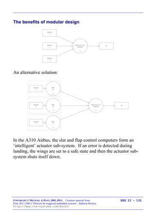
Example: Fail-Silent behaviour in the Airbus A310
In the A310 Airbus, the slat and flap control computers form
an „intelligent‟ actuator sub-system.
If an error is detected during landing, the wings are set to a
safe state and then the actuator sub-system shuts itself down
(Burns and Wellings, 1997, p.102).
[Please note that the mechanisms underlying this “fail silent”
behaviour are unknown.]](https://image.slidesharecdn.com/programmingembeddedsystemsii-200229112938/85/Programming-embedded-systems-ii-129-320.jpg)
![COPYRIGHT © MICHAEL J. PONT, 2001-2011. Contains material from:
Pont, M.J. (2001) “Patterns for triggered embedded systems”, Addison-Wesley.
http://www.tte-systems.com/books
PES II - 117
Example: Fail-Silent behaviour in a steer-by-wire application
Suppose that an automotive steer-by-wire system has been created
that runs a single task, every 10 ms. We will assume that the
system is being monitored to check for task over-runs (see
SCHEDULER WATCHDOG [this seminar]). We will also assume that
the system has been well designed, and has appropriate timeout
code, etc, implemented.
Further suppose that a passenger car using this system is being
driven on a motorway, and that an error is detected, resulting in a
watchdog reset. What recovery behaviour should be implemented?
We could simply re-start the scheduler and “hope for the best”.
However, this form of “reset recovery” is probably not appropriate.
In this case, if we simply perform a reset, we may leave the driver
without control of their vehicle (see RESET RECOVERY [this
seminar]).
Instead, we could implement a fail-silent strategy. In this case, we
would simply aim to bring the vehicle, slowly, to a halt. To warn
other road vehicles that there was a problem, we could choose to
flash all the lights on the vehicle on an off (continuously), and to
pulse the horn. This strategy (which may - in fact - be far from
silent) is not ideal, because there can be no guarantee that the driver
and passengers (or other road vehicles) will survive the incident.
However, it the event of a very serious system failure, it may be all
that we can do.](https://image.slidesharecdn.com/programmingembeddedsystemsii-200229112938/85/Programming-embedded-systems-ii-130-320.jpg)
![COPYRIGHT © MICHAEL J. PONT, 2001-2011. Contains material from:
Pont, M.J. (2001) “Patterns for triggered embedded systems”, Addison-Wesley.
http://www.tte-systems.com/books
PES II - 119
Example: Limp-home behaviour in a steer-by-wire
application
In FAIL-SILENT RECOVERY [this seminar], we considered one
possible recovery strategy in a steer-by-sire application.
As an alternative to the approach discussed in the previous example,
we may wish to consider a limp-home control strategy. In this case,
a suitable strategy might involve a code structure like this:
while(1)
{
Update_basic_steering_control();
Software_delay_10ms();
}
This is a basic software architecture (based on SUPER LOOP
[PTTES, p.162]).
In creating this version, we have avoided use of the scheduler code.
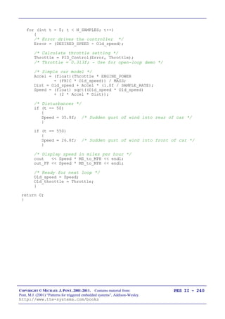
We might also wish to use a different (simpler) control algorithm at
the heart of this system. For example, the main control algorithm
may use measurements of the current speed, in order to ensure a
smooth response even when the vehicle is moving rapidly. We
could omit this feature in the “limp home” version.](https://image.slidesharecdn.com/programmingembeddedsystemsii-200229112938/85/Programming-embedded-systems-ii-132-320.jpg)
![COPYRIGHT © MICHAEL J. PONT, 2001-2011. Contains material from:
Pont, M.J. (2001) “Patterns for triggered embedded systems”, Addison-Wesley.
http://www.tte-systems.com/books
PES II - 129
P 2.7 (A15) 28
P 2.6 (A14) 27
P 2.5 (A13) 26
P 2.4 (A12) 25
P 2.3 (A11) 24
P 2.2 (A10) 23
P 2.1 (A9) 22
P 2.0 (A8) 21
ALE (/PROG)
/ EA
/PSEN
31
30
29
19 XTL1
XTL218
RST9
40
VCC
20
VSS
“8051”
P 1.7
1
2
3
4
5
P 1.56
7
P 1.0 [T2]
P 1.1 [T2EX]
P 1.2
P 1.3
P 1.4
P 1.6
8
P 3.0 (RXD)
P 3.1 (TXD)
P 3.2 (/INT0)
P 3.3 (/INT1)
P 3.4 (T0)
P 3.5 (T1)
P 3.6 (/WR)
P 3.7 (/RD)
10
11
12
13
14
15
16
17
P 0.0 (AD0) 39
P 0.1 (AD1) 38
P 0.2 (AD2) 37
P 0.3 (AD3) 36
P 0.4 (AD4) 35
P 0.5 (AD5) 34
P 0.6 (AD6) 33
P 0.7 (AD7) 32
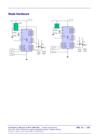
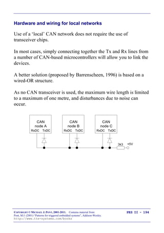
A flexible environment with 62 free port pins, 5 free timers,
two UARTs, etc.
Further microcontrollers may be added without difficulty,
The communication over a single wire (plus ground) will
ensure that the tasks on all processors are synchronised.
The two-microcontroller design also has two CPUs:
true multi-tasking is possibly.](https://image.slidesharecdn.com/programmingembeddedsystemsii-200229112938/85/Programming-embedded-systems-ii-142-320.jpg)

![COPYRIGHT © MICHAEL J. PONT, 2001-2011. Contains material from:
Pont, M.J. (2001) “Patterns for triggered embedded systems”, Addison-Wesley.
http://www.tte-systems.com/books
PES II - 170
RS-232 vs RS-485 [number of nodes]
RS-232 is a peer-to-peer communications standard. For our
purposes, this means that it is suitable for applications that
involve two nodes, each containing a microcontroller (or, as
we saw in PTTES, Chapter 18, for applications where one
node is a desktop, or similar, PC).
RS-485 is a „multi-point‟ or „multi-drop‟ communications
standard. For our purposes, this means applications that
involve at least three nodes, each containing a
microcontroller. Larger RS-485 networks can have up to 32
„unit loads‟: by using high-impedance receivers, you can
have as many as 256 nodes on the network.](https://image.slidesharecdn.com/programmingembeddedsystemsii-200229112938/85/Programming-embedded-systems-ii-183-320.jpg)
![COPYRIGHT © MICHAEL J. PONT, 2001-2011. Contains material from:
Pont, M.J. (2001) “Patterns for triggered embedded systems”, Addison-Wesley.
http://www.tte-systems.com/books
PES II - 171
RS-232 vs RS-485 [range and baud rates]
RS-232 is a single-wire standard (one signal line, per
channel, plus ground). Electrical noise in the environment
can lead to data corruption. This restricts the
communication range to a maximum of around 30 metres,
and the data rate to around 115 kbaud (with recent drivers).
RS-485 is a two-wire or differential communication
standard. This means that, for each channel, two lines carry
(1) the required signal and (2) the inverse of the signal. The
receiver then detects the voltage difference between the two
lines. Electrical noise will impact on both lines, and will
cancel out when the difference is calculated at the receiver.
As a result, an RS-485 network can extend as far as 1 km, at
a data rate of 90 kbaud. Faster data rates (up to 10 Mbaud)
are possible at shorter distances (up to 15 metres).](https://image.slidesharecdn.com/programmingembeddedsystemsii-200229112938/85/Programming-embedded-systems-ii-184-320.jpg)
![COPYRIGHT © MICHAEL J. PONT, 2001-2011. Contains material from:
Pont, M.J. (2001) “Patterns for triggered embedded systems”, Addison-Wesley.
http://www.tte-systems.com/books
PES II - 172
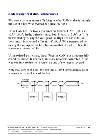
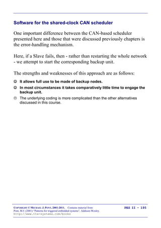
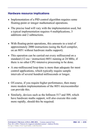
RS-232 vs RS-485 [cabling]
RS-232 requires low-cost „straight‟ cables, with three wires
for fully duplex communications (Tx, Rx, Ground).
For full performance, RS-485 requires twisted-pair cables,
with two twisted pairs, plus ground (and usually a screen).
This cabling is more bulky and more expensive than the RS-
232 equivalent.
RS-232 cables do not require terminating resistors.
RS-485 cables are usually used with 120 terminating
resistors (assuming 24-AWG twisted pair cables) connected
in parallel, at or just beyond the final node at both ends of
the network. The terminations reduce voltage reflections
that can otherwise cause the receiver to misread logic levels.
120120
Slave 1Slave 1MASTERMASTER Slave 2Slave 2
120120
RS-485 Gnd
100 100100](https://image.slidesharecdn.com/programmingembeddedsystemsii-200229112938/85/Programming-embedded-systems-ii-185-320.jpg)
![COPYRIGHT © MICHAEL J. PONT, 2001-2011. Contains material from:
Pont, M.J. (2001) “Patterns for triggered embedded systems”, Addison-Wesley.
http://www.tte-systems.com/books
PES II - 173
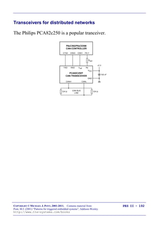
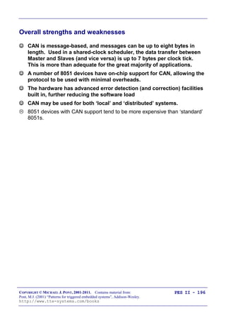
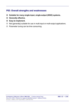
RS-232 vs RS-485 [transceivers]
RS-232 transceivers are simple and standard.
Choice of RS-485 transceivers depends on the application.
A common choice for basic systems is the Maxim Max489
family. For increased reliability, the Linear Technology
LTC1482, National Semiconductors DS36276 and the
Maxim MAX3080–89 series all have internal circuitry to
protect against cable short circuits. Also, the Maxim Max
MAX1480 contains its own transformer-isolated supply and
opto-isolated signal path: this can help avoid interaction
between power lines and network cables destroying your
microcontroller.
P 0.7 (AD7)
32
P 0.6 (AD6) 33
P 0.5 (AD5)
34
P 0.4 (AD4) 35
P 0.3 (AD3)
36
P 0.2 (AD2) 37
P 0.1 (AD1) 38
P 0.0 (AD0) 39
8
7
6
5
4
3
2
1
P 2.7 (A15) 28
P 2.6 (A14) 27
P 2.5 (A13) 26
P 2.4 (A12) 25
P 2.3 (A11)
24
P 2.2 (A10)
23
P 2.1 (A9)
22
P 2.0 (A8)
21
/ PSEN
ALE (/ PROG)
29
30
31
XTL1
19
XTL2
18
RST
40
VCC
VSS
AT89S53
Vcc (+5V)
Vcc
Cxtal
Cxtal
Creset
Rreset
20
P 3.7 (/ RD)
P 3.6 (/ WR)
P 3.5 (T1)
P 3.4 (T0)
P 3.3 (/ INT1)
P 3.2 (/ INT 0)
P 3.1 (TXD)
P 3.0 (RXD)
/ EA
17
16
15
14
13
12
11
10
9
Vcc
Max
489 5
2
485-IA
485-IB
485-OA
485-OB
14
12
11
9
10
3
6,7
485-GND
100 R
4
P 1.7 (SCK)
P 1.6 (MISO)
P 1.5 (MOSI)
P 1.4(/SS)
P 1.3
P 1.2
P 1.1 (T2EX)
P 1.0 (T2)](https://image.slidesharecdn.com/programmingembeddedsystemsii-200229112938/85/Programming-embedded-systems-ii-186-320.jpg)


![COPYRIGHT © MICHAEL J. PONT, 2001-2011. Contains material from:
Pont, M.J. (2001) “Patterns for triggered embedded systems”, Addison-Wesley.
http://www.tte-systems.com/books
PES II - 198
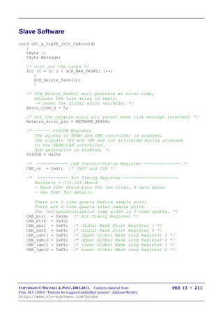
Master Software
void SCC_A_MASTER_Init_T2_CAN(void)
{
tByte i;
tByte Message;
tByte Slave_index;
EA = 0; /* No interrupts (yet) */
SCC_A_MASTER_Watchdog_Init(); /* Start the watchdog */
Network_error_pin = NO_NETWORK_ERROR;
for (i = 0; i < SCH_MAX_TASKS; i++)
{
SCH_Delete_Task(i); /* Clear the task array */
}
/* SCH_Delete_Task() will generate an error code,
because the task array is empty.
-> reset the global error variable. */
Error_code_G = 0;
/* We allow any combination of ID numbers in slaves */
for (Slave_index =0; Slave_index < NUMBER_OF_SLAVES; Slave_index++)
{
Slave_reset_attempts_G[Slave_index] = 0;
Current_Slave_IDs_G[Slave_index] = MAIN_SLAVE_IDs[Slave_index];
}
/* Get ready to send first tick message */
First_ack_G = 1;
Slave_index_G = 0;
/* ------ Set up the CAN link (begin) ------------------------ */
/* ---------------- SYSCON Register --------------
The access to XRAM and CAN controller is enabled.
The signals !RD and !WR are not activated during accesses
to the XRAM/CAN controller.
ALE generation is enabled. */
SYSCON = 0x20;
/* ------------ CAN Control/Status Register --------------
Start to init the CAN module. */
CAN_cr = 0x41; /* INIT and CCE */](https://image.slidesharecdn.com/programmingembeddedsystemsii-200229112938/85/Programming-embedded-systems-ii-211-320.jpg)
![COPYRIGHT © MICHAEL J. PONT, 2001-2011. Contains material from:
Pont, M.J. (2001) “Patterns for triggered embedded systems”, Addison-Wesley.
http://www.tte-systems.com/books
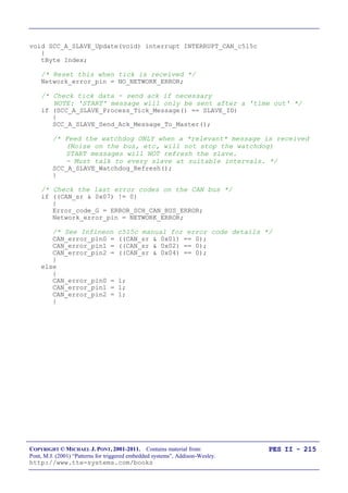
PES II - 199
/* ------------ Bit Timing Register ---------------------
Baudrate = 333.333 kbaud
- Need 308+ kbaud plus for 1ms ticks, 8 data bytes
- See text for details
There are 5 time quanta before sample point
There are 4 time quanta after sample point
The (re)synchronization jump width is 2 time quanta. */
CAN_btr1 = 0x34; /* Bit Timing Register */
CAN_btr0 = 0x42;
CAN_gms1 = 0xFF; /* Global Mask Short Register 1 */
CAN_gms0 = 0xFF; /* Global Mask Short Register 0 */
CAN_ugml1 = 0xFF; /* Upper Global Mask Long Register 1 */
CAN_ugml0 = 0xFF; /* Upper Global Mask Long Register 0 */
CAN_lgml1 = 0xF8; /* Lower Global Mask Long Register 1 */
CAN_lgml0 = 0xFF; /* Lower Global Mask Long Register 0 */
/* --- Configure the 'Tick' Message Object --- */
/* 'Message Object 1' is valid */
CAN_messages[0].MCR1 = 0x55; /* Message Control Register 1 */
CAN_messages[0].MCR0 = 0x95; /* Message Control Register 0 */
/* Message direction is transmit
Extended 29-bit identifier
These have ID 0x000000 and 5 valid data bytes. */
CAN_messages[0].MCFG = 0x5C; /* Message Config Reg */
CAN_messages[0].UAR1 = 0x00; /* Upper Arbit. Reg. 1 */
CAN_messages[0].UAR0 = 0x00; /* Upper Arbit. Reg. 0 */
CAN_messages[0].LAR1 = 0x00; /* Lower Arbit. Reg. 1 */
CAN_messages[0].LAR0 = 0x00; /* Lower Arbit. Reg. 0 */
CAN_messages[0].Data[0] = 0x00; /* Data byte 0 */
CAN_messages[0].Data[1] = 0x00; /* Data byte 1 */
CAN_messages[0].Data[2] = 0x00; /* Data byte 2 */
CAN_messages[0].Data[3] = 0x00; /* Data byte 3 */
CAN_messages[0].Data[4] = 0x00; /* Data byte 4 */](https://image.slidesharecdn.com/programmingembeddedsystemsii-200229112938/85/Programming-embedded-systems-ii-212-320.jpg)
![COPYRIGHT © MICHAEL J. PONT, 2001-2011. Contains material from:
Pont, M.J. (2001) “Patterns for triggered embedded systems”, Addison-Wesley.
http://www.tte-systems.com/books
PES II - 200
/* --- Configure the 'Ack' Message Object --- */
/* 'Message Object 2' is valid
NOTE: Object 2 receives *ALL* ack messages. */
CAN_messages[1].MCR1 = 0x55; /* Message Control Register 1 */
CAN_messages[1].MCR0 = 0x95; /* Message Control Register 0 */
/* Message direction is receive
Extended 29-bit identifier
These all have ID: 0x000000FF (5 valid data bytes) */
CAN_messages[1].MCFG = 0x04; /* Message Config Reg */
CAN_messages[1].UAR1 = 0x00; /* Upper Arbit. Reg. 1 */
CAN_messages[1].UAR0 = 0x00; /* Upper Arbit. Reg. 0 */
CAN_messages[1].LAR1 = 0xF8; /* Lower Arbit. Reg. 1 */
CAN_messages[1].LAR0 = 0x07; /* Lower Arbit. Reg. 0 */
/* Configure remaining message objects - none is valid */
for (Message = 2; Message <= 14; ++Message)
{
CAN_messages[Message].MCR1 = 0x55; /* Message Control Reg 1 */
CAN_messages[Message].MCR0 = 0x55; /* Message Control Reg 0 */
}
/* ------------ CAN Control Register --------------------- */
/* Reset CCE and INIT */
CAN_cr = 0x00;
/* ------ Set up the CAN link (end) ---------------------- */](https://image.slidesharecdn.com/programmingembeddedsystemsii-200229112938/85/Programming-embedded-systems-ii-213-320.jpg)
![COPYRIGHT © MICHAEL J. PONT, 2001-2011. Contains material from:
Pont, M.J. (2001) “Patterns for triggered embedded systems”, Addison-Wesley.
http://www.tte-systems.com/books
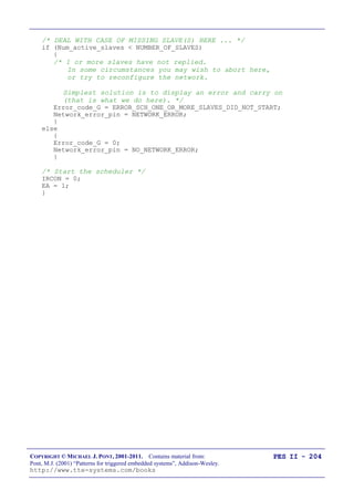
PES II - 203
/* After the initial (long) delay, all slaves will have timed out.
All operational slaves will now be in the 'READY TO START' state
Send them a 'slave id' message to get them started. */
Slave_index = 0;
do {
/* Refresh the watchdog */
SCC_A_MASTER_Watchdog_Refresh();
/* Find the slave ID for this slave */
Slave_ID = (tByte) Current_Slave_IDs_G[Slave_index];
Slave_replied_correctly = SCC_A_MASTER_Start_Slave(Slave_ID);
if (Slave_replied_correctly)
{
Num_active_slaves++;
Slave_index++;
}
else
{
/* Slave did not reply correctly
- try to switch to backup device (if available) */
if (Current_Slave_IDs_G[Slave_index] !=
BACKUP_SLAVE_IDs[Slave_index])
{
/* A backup is available: switch to it and re-try */
Current_Slave_IDs_G[Slave_index]
= BACKUP_SLAVE_IDs[Slave_index];
}
else
{
/* No backup available (or backup failed too)
- have to continue */
Slave_index++;
}
}
} while (Slave_index < NUMBER_OF_SLAVES);](https://image.slidesharecdn.com/programmingembeddedsystemsii-200229112938/85/Programming-embedded-systems-ii-216-320.jpg)
![COPYRIGHT © MICHAEL J. PONT, 2001-2011. Contains material from:
Pont, M.J. (2001) “Patterns for triggered embedded systems”, Addison-Wesley.
http://www.tte-systems.com/books
PES II - 205
void SCC_A_MASTER_Update_T2(void) interrupt INTERRUPT_Timer_2_Overflow
{
tByte Index;
tByte Previous_slave_index;
bit Slave_replied_correctly;
TF2 = 0; /* Must clear this. */
/* Refresh the watchdog */
SCC_A_MASTER_Watchdog_Refresh();
/* Default */
Network_error_pin = NO_NETWORK_ERROR;
/* Keep track of the current slave
(First value of "prev slave" is 0) */
Previous_slave_index = Slave_index_G
if (++Slave_index_G >= NUMBER_OF_SLAVES)
{
Slave_index_G = 0;
}
/* Check that the approp slave replied to the last message.
(If it did, store the data sent by this slave) */
if (SCC_A_MASTER_Process_Ack(Previous_slave_index) == RETURN_ERROR)
{
Error_code_G = ERROR_SCH_LOST_SLAVE;
Network_error_pin = NETWORK_ERROR;
/* If we have lost contact with a slave, we attempt to
switch to a backup device (if one is available) */
if (Current_Slave_IDs_G[Slave_index_G] !=
BACKUP_SLAVE_IDs[Slave_index_G])
{
/* A backup is available: switch to it and re-try */
Current_Slave_IDs_G[Slave_index_G] =
BACKUP_SLAVE_IDs[Slave_index_G];
}
else
{
/* There is no backup available (or we are already using it).
Try main device again. */
Current_Slave_IDs_G[Slave_index_G] =
MAIN_SLAVE_IDs[Slave_index_G];
}](https://image.slidesharecdn.com/programmingembeddedsystemsii-200229112938/85/Programming-embedded-systems-ii-218-320.jpg)
![COPYRIGHT © MICHAEL J. PONT, 2001-2011. Contains material from:
Pont, M.J. (2001) “Patterns for triggered embedded systems”, Addison-Wesley.
http://www.tte-systems.com/books
PES II - 206
/* Try to connect to the slave */
Slave_replied_correctly =
SCC_A_MASTER_Start_Slave(Current_Slave_IDs_G[Slave_index_G]);
if (!Slave_replied_correctly)
{
/* No backup available (or it failed too) - we shut down
(OTHER ACTIONS MAY BE MORE APPROPRIATE IN YOUR SYSTEM!) */
SCC_A_MASTER_Shut_Down_the_Network();
}
}
/* Send 'tick' message to all connected slaves
(sends one data byte to the current slave). */
SCC_A_MASTER_Send_Tick_Message(Slave_index_G);
/* Check the last error codes on the CAN bus */
if ((CAN_sr & 0x07) != 0)
{
Error_code_G = ERROR_SCH_CAN_BUS_ERROR;
Network_error_pin = NETWORK_ERROR;
/* See Infineon C515C manual for error code details */
CAN_error_pin0 = ((CAN_sr & 0x01) == 0);
CAN_error_pin1 = ((CAN_sr & 0x02) == 0);
CAN_error_pin2 = ((CAN_sr & 0x04) == 0);
}
else
{
CAN_error_pin0 = 1;
CAN_error_pin1 = 1;
CAN_error_pin2 = 1;
}](https://image.slidesharecdn.com/programmingembeddedsystemsii-200229112938/85/Programming-embedded-systems-ii-219-320.jpg)
![COPYRIGHT © MICHAEL J. PONT, 2001-2011. Contains material from:
Pont, M.J. (2001) “Patterns for triggered embedded systems”, Addison-Wesley.
http://www.tte-systems.com/books
PES II - 207
/* NOTE: calculations are in *TICKS* (not milliseconds) */
for (Index = 0; Index < SCH_MAX_TASKS; Index++)
{
/* Check if there is a task at this location */
if (SCH_tasks_G[Index].pTask)
{
if (SCH_tasks_G[Index].Delay == 0)
{
/* The task is due to run */
SCH_tasks_G[Index].RunMe += 1; /* Inc RunMe */
if (SCH_tasks_G[Index].Period)
{
/* Schedule periodic tasks to run again */
SCH_tasks_G[Index].Delay = SCH_tasks_G[Index].Period;
}
}
else
{
/* Not yet ready to run: just decrement the delay */
SCH_tasks_G[Index].Delay -= 1;
}
}
}
}](https://image.slidesharecdn.com/programmingembeddedsystemsii-200229112938/85/Programming-embedded-systems-ii-220-320.jpg)
![COPYRIGHT © MICHAEL J. PONT, 2001-2011. Contains material from:
Pont, M.J. (2001) “Patterns for triggered embedded systems”, Addison-Wesley.
http://www.tte-systems.com/books
PES II - 208
void SCC_A_MASTER_Send_Tick_Message(const tByte SLAVE_INDEX)
{
/* Find the slave ID for this slave
ALL SLAVES MUST HAVE A UNIQUE (non-zero) ID! */
tByte Slave_ID = (tByte) Current_Slave_IDs_G[SLAVE_INDEX];
CAN_messages[0].Data[0] = Slave_ID;
/* Fill the data fields */
CAN_messages[0].Data[1] = Tick_message_data_G[SLAVE_INDEX][0];
CAN_messages[0].Data[2] = Tick_message_data_G[SLAVE_INDEX][1];
CAN_messages[0].Data[3] = Tick_message_data_G[SLAVE_INDEX][2];
CAN_messages[0].Data[4] = Tick_message_data_G[SLAVE_INDEX][3];
/* Send the message on the CAN bus */
CAN_messages[0].MCR1 = 0xE7; /* TXRQ, reset CPUUPD */
}](https://image.slidesharecdn.com/programmingembeddedsystemsii-200229112938/85/Programming-embedded-systems-ii-221-320.jpg)
![COPYRIGHT © MICHAEL J. PONT, 2001-2011. Contains material from:
Pont, M.J. (2001) “Patterns for triggered embedded systems”, Addison-Wesley.
http://www.tte-systems.com/books
PES II - 209
bit SCC_A_MASTER_Process_Ack(const tByte SLAVE_INDEX)
{
tByte Ack_ID, Slave_ID;
/* First time this is called there is no Ack message to check
- we simply return 'OK'. */
if (First_ack_G)
{
First_ack_G = 0;
return RETURN_NORMAL;
}
if ((CAN_messages[1].MCR1 & 0x03) == 0x02) /* if NEWDAT */
{
/* An ack message was received
-> extract the data */
Ack_ID = CAN_messages[1].Data[0]; /* Get data byte 0 */
Ack_message_data_G[SLAVE_INDEX][0] = CAN_messages[1].Data[1];
Ack_message_data_G[SLAVE_INDEX][1] = CAN_messages[1].Data[2];
Ack_message_data_G[SLAVE_INDEX][2] = CAN_messages[1].Data[3];
Ack_message_data_G[SLAVE_INDEX][3] = CAN_messages[1].Data[4];
CAN_messages[1].MCR0 = 0xfd; /* reset NEWDAT, INTPND */
CAN_messages[1].MCR1 = 0xfd;
/* Find the slave ID for this slave */
Slave_ID = (tByte) Current_Slave_IDs_G[SLAVE_INDEX];
if (Ack_ID == Slave_ID)
{
return RETURN_NORMAL;
}
}
/* No message, or ID incorrect */
return RETURN_ERROR;
}](https://image.slidesharecdn.com/programmingembeddedsystemsii-200229112938/85/Programming-embedded-systems-ii-222-320.jpg)
![COPYRIGHT © MICHAEL J. PONT, 2001-2011. Contains material from:
Pont, M.J. (2001) “Patterns for triggered embedded systems”, Addison-Wesley.
http://www.tte-systems.com/books
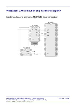
PES II - 212
/* ------ Configure 'Tick' Message Object */
/* Message object 1 is valid */
/* Enable receive interrupt */
CAN_messages[0].MCR1 = 0x55; /* Message Ctrl. Reg. 1 */
CAN_messages[0].MCR0 = 0x99; /* Message Ctrl. Reg. 0 */
/* message direction is receive */
/* extended 29-bit identifier */
CAN_messages[0].MCFG = 0x04; /* Message Config. Reg. */
CAN_messages[0].UAR1 = 0x00; /* Upper Arbit. Reg. 1 */
CAN_messages[0].UAR0 = 0x00; /* Upper Arbit. Reg. 0 */
CAN_messages[0].LAR1 = 0x00; /* Lower Arbit. Reg. 1 */
CAN_messages[0].LAR0 = 0x00; /* Lower Arbit. Reg. 0 */
/* ------ Configure 'Ack' Message Object */
CAN_messages[1].MCR1 = 0x55; /* Message Ctrl. Reg. 1 */
CAN_messages[1].MCR0 = 0x95; /* Message Ctrl. Reg. 0 */
/* Message direction is transmit */
/* Extended 29-bit identifier; 5 valid data bytes */
CAN_messages[1].MCFG = 0x5C; /* Message Config. Reg. */
CAN_messages[1].UAR1 = 0x00; /* Upper Arbit. Reg. 1 */
CAN_messages[1].UAR0 = 0x00; /* Upper Arbit. Reg. 0 */
CAN_messages[1].LAR1 = 0xF8; /* Lower Arbit. Reg. 1 */
CAN_messages[1].LAR0 = 0x07; /* Lower Arbit. Reg. 0 */
CAN_messages[1].Data[0] = 0x00; /* Data byte 0 */
CAN_messages[1].Data[1] = 0x00; /* Data byte 1 */
CAN_messages[1].Data[2] = 0x00; /* Data byte 2 */
CAN_messages[1].Data[3] = 0x00; /* Data byte 3 */
CAN_messages[1].Data[4] = 0x00; /* Data byte 4 */
/* ------ Configure other objects --------------------------- */
/* Configure remaining message objects (2-14) - none is valid */
for (Message = 2; Message <= 14; ++Message)
{
CAN_messages[Message].MCR1 = 0x55; /* Message Ctrl. Reg. 1 */
CAN_messages[Message].MCR0 = 0x55; /* Message Ctrl. Reg. 0 */
}
/* ------------ CAN Ctrl. Reg. --------------------- */
/* Reset CCE and INIT */
/* Enable interrupt generation from CAN Modul */
/* Enable CAN-interrupt of Controller */
CAN_cr = 0x02;
IEN2 |= 0x02;
SCC_A_SLAVE_Watchdog_Init(); /* Start the watchdog */
}](https://image.slidesharecdn.com/programmingembeddedsystemsii-200229112938/85/Programming-embedded-systems-ii-225-320.jpg)
![COPYRIGHT © MICHAEL J. PONT, 2001-2011. Contains material from:
Pont, M.J. (2001) “Patterns for triggered embedded systems”, Addison-Wesley.
http://www.tte-systems.com/books
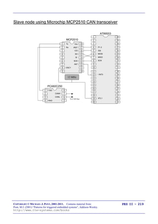
PES II - 213
void SCC_A_SLAVE_Start(void)
{
tByte Tick_00, Tick_ID;
bit Start_slave;
/* Disable interrupts */
EA = 0;
/* We can be at this point because:
1. The network has just been powered up
2. An error has occurred in the Master, and it is not gen. ticks
3. The network has been damaged -> no ticks are being recv
Try to make sure the system is in a safe state...
NOTE: Interrupts are disabled here!! */
SCC_A_SLAVE_Enter_Safe_State();
Start_slave = 0;
Error_code_G = ERROR_SCH_WAITING_FOR_START_COMMAND_FROM_MASTER;
SCH_Report_Status(); /* Sch not yet running - do this manually */
/* Now wait (indefinitely) for approp signal from the Master */
do {
/* Wait for 'Slave ID' message to be received */
do {
SCC_A_SLAVE_Watchdog_Refresh(); /* Must feed watchdog */
} while ((CAN_messages[0].MCR1 & 0x03) != 0x02);
/* Got a message - extract the data */
if ((CAN_messages[0].MCR1 & 0x0c) == 0x08) /* if MSGLST set */
{
/* Ignore lost message */
CAN_messages[0].MCR1 = 0xf7; /* reset MSGLST */
}
Tick_00 = (tByte) CAN_messages[0].Data[0]; /* Get Data 0 */
Tick_ID = (tByte) CAN_messages[0].Data[1]; /* Get Data 1 */
CAN_messages[0].MCR0 = 0xfd; /* reset NEWDAT, INTPND */
CAN_messages[0].MCR1 = 0xfd;](https://image.slidesharecdn.com/programmingembeddedsystemsii-200229112938/85/Programming-embedded-systems-ii-226-320.jpg)
![COPYRIGHT © MICHAEL J. PONT, 2001-2011. Contains material from:
Pont, M.J. (2001) “Patterns for triggered embedded systems”, Addison-Wesley.
http://www.tte-systems.com/books
PES II - 214
if ((Tick_00 == 0x00) && (Tick_ID == SLAVE_ID))
{
/* Message is correct */
Start_slave = 1;
/* Send ack */
CAN_messages[1].Data[0] = 0x00; /* Set data byte 0 */
CAN_messages[1].Data[1] = SLAVE_ID; /* Set data byte 1 */
CAN_messages[1].MCR1 = 0xE7; /* Send message */
}
else
{
/* Not yet received correct message - wait */
Start_slave = 0;
}
} while (!Start_slave);
/* Start the scheduler */
IRCON = 0;
EA = 1;
}](https://image.slidesharecdn.com/programmingembeddedsystemsii-200229112938/85/Programming-embedded-systems-ii-227-320.jpg)
![COPYRIGHT © MICHAEL J. PONT, 2001-2011. Contains material from:
Pont, M.J. (2001) “Patterns for triggered embedded systems”, Addison-Wesley.
http://www.tte-systems.com/books
PES II - 216
/* NOTE: calculations are in *TICKS* (not milliseconds) */
for (Index = 0; Index < SCH_MAX_TASKS; Index++)
{
/* Check if there is a task at this location */
if (SCH_tasks_G[Index].pTask)
{
if (SCH_tasks_G[Index].Delay == 0)
{
/* The task is due to run */
SCH_tasks_G[Task_index].RunMe += 1; /* Inc RunMe */
if (SCH_tasks_G[Task_index].Period)
{
/* Schedule periodic tasks to run again */
SCH_tasks_G[Task_index].Delay =
SCH_tasks_G[Task_index].Period;
}
}
else
{
/* Not yet ready to run: just decrement the delay */
SCH_tasks_G[Index].Delay -= 1;
}
}
}
}](https://image.slidesharecdn.com/programmingembeddedsystemsii-200229112938/85/Programming-embedded-systems-ii-229-320.jpg)
![COPYRIGHT © MICHAEL J. PONT, 2001-2011. Contains material from:
Pont, M.J. (2001) “Patterns for triggered embedded systems”, Addison-Wesley.
http://www.tte-systems.com/books
PES II - 217
tByte SCC_A_SLAVE_Process_Tick_Message(void)
{
tByte Tick_ID;
if ((CAN_messages[0].MCR1 & 0x0c) == 0x08) /* If MSGLST set */
{
/* The CAN controller has stored a new
message into this object, while NEWDAT was still set,
i.e. the previously stored message is lost.
We simply IGNORE this here and reset the flag. */
CAN_messages[0].MCR1 = 0xf7; /* reset MSGLST */
}
/* The first byte is the ID of the slave
for which the data are intended. */
Tick_ID = CAN_messages[0].Data[0]; /* Get Slave ID */
if (Tick_ID == SLAVE_ID)
{
/* Only if there is a match do we need to copy these fields */
Tick_message_data_G[0] = CAN_messages[0].Data[1];
Tick_message_data_G[1] = CAN_messages[0].Data[2];
Tick_message_data_G[2] = CAN_messages[0].Data[3];
Tick_message_data_G[3] = CAN_messages[0].Data[4];
}
CAN_messages[0].MCR0 = 0xfd; /* reset NEWDAT, INTPND */
CAN_messages[0].MCR1 = 0xfd;
return Tick_ID;
}
void SCC_A_SLAVE_Send_Ack_Message_To_Master(void)
{
/* First byte of message must be slave ID */
CAN_messages[1].Data[0] = SLAVE_ID; /* data byte 0 */
CAN_messages[1].Data[1] = Ack_message_data_G[0];
CAN_messages[1].Data[2] = Ack_message_data_G[1];
CAN_messages[1].Data[3] = Ack_message_data_G[2];
CAN_messages[1].Data[4] = Ack_message_data_G[3];
/* Send the message on the CAN bus */
CAN_messages[1].MCR1 = 0xE7; /* TXRQ, reset CPUUPD */
}](https://image.slidesharecdn.com/programmingembeddedsystemsii-200229112938/85/Programming-embedded-systems-ii-230-320.jpg)


![COPYRIGHT © MICHAEL J. PONT, 2001-2011. Contains material from:
Pont, M.J. (2001) “Patterns for triggered embedded systems”, Addison-Wesley.
http://www.tte-systems.com/books
PES II - 237
Why open-loop controllers are still (sometimes) useful
Open-loop control still has a role to play.
For example, if we wish to control the speed of an electric
fan in an automotive air-conditioning system, we may not
need precise speed control, and an open-loop approach
might be appropriate.
In addition, it is not always possible to directly measure the
quantity we are trying to control, making closed-loop
control impractical.
For example, in an insulin delivery system used for patients
with diabetes, we are seeking to control levels of glucose in
the bloodstream. However, glucose sensors are not
available, so an open-loop controller must be used; please
see Dorf and Bishop (1998, p. 22) for further details.
[Similar problems apply throughout much of the process
industry, where sensors are not available to determine
product quality.]](https://image.slidesharecdn.com/programmingembeddedsystemsii-200229112938/85/Programming-embedded-systems-ii-250-320.jpg)
![COPYRIGHT © MICHAEL J. PONT, 2001-2011. Contains material from:
Pont, M.J. (2001) “Patterns for triggered embedded systems”, Addison-Wesley.
http://www.tte-systems.com/books
PES II - 239
Example: Tuning the parameters of a cruise-control system
In this example, we take a simple computer simulation of a vehicle,
and develop an appropriate cruise-control system to match.
#include <iostream.h>
#include <fstream.h>
#include <math.h>
#include "PID_f.h"
/* ------ Private constants --------------------------------------- */
#define MS_to_MPH (2.2369) /* Convert metres/sec to mph */
#define FRIC (50) /* Friction coeff- Newton Second / m */
#define MASS (1000) /* Mass of vehicle (kgs) */
#define N_SAMPLES (1000) /* Number of samples */
#define ENGINE_POWER (5000) /* N */
#define DESIRED_SPEED (31.3f) /* Metres/sec [* 2.2369 -> mph] */
int main()
{
float Throttle = 0.313f; /* Throttle setting (fraction) */
float Old_speed = DESIRED_SPEED, Old_throttle = 0.313f;
float Error, Speed, Accel, Dist;
float Sum = 0.0f;
/* Open file to store results */
fstream out_FP;
out_FP. open("pid.txt", ios::out);
if (!out_FP)
{
cerr << "ERROR: Cannot open an essential file.";
return 1;
}](https://image.slidesharecdn.com/programmingembeddedsystemsii-200229112938/85/Programming-embedded-systems-ii-252-320.jpg)
![COPYRIGHT © MICHAEL J. PONT, 2001-2011. Contains material from:
Pont, M.J. (2001) “Patterns for triggered embedded systems”, Addison-Wesley.
http://www.tte-systems.com/books
PES II - 241
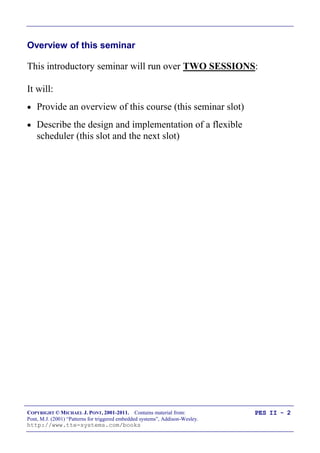
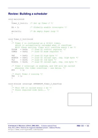
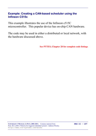
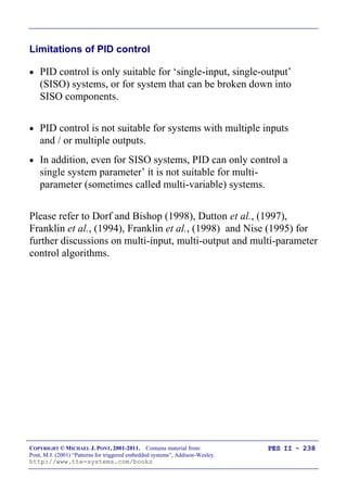
Open-loop test
55
65
75
85
1
29
57
85
113
141
169
197
225
253
281
309
337
365
393
421
449
477
505
533
561
589
617
645
673
701
729
757
785
813
841
869
897
925
953
981
[NO CONTROLLER - open loop]
Time (Seconds)
Speed (mph)
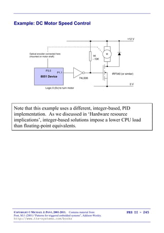
The car is controlled by maintaining a fixed throttle position
at all times. Because we assume the vehicle is driving on a
straight, flat, road with no wind, the speed is constant (70
mph) for most of the 1000-second trip.
At time t = 50 seconds, we simulate a sudden gust of wind at
the rear of the car; this speeds the vehicle up, and it slowly
returns to the set speed value.
At time t = 550 seconds, we simulate a sharp gust of wind at
the front of the car; this slows the vehicle down.](https://image.slidesharecdn.com/programmingembeddedsystemsii-200229112938/85/Programming-embedded-systems-ii-254-320.jpg)
![COPYRIGHT © MICHAEL J. PONT, 2001-2011. Contains material from:
Pont, M.J. (2001) “Patterns for triggered embedded systems”, Addison-Wesley.
http://www.tte-systems.com/books
PES II - 247
void PID_MOTOR_Control_Motor(void)
{
int Error, Control_new;
Speed_measured_G = PID_MOTOR_Read_Current_Speed();
Speed_required_G = PID_MOTOR_Get_Required_Speed();
/* Difference between required and actual speed (0-255) */
Error = Speed_required_G - Speed_measured_G;
/* Proportional term */
Control_new = Controller_output_G + (Error / PID_PROPORTIONAL);
/* Integral term [SET TO 0 IF NOT REQUIRED] */
if (PID_INTEGRAL)
{
Sum_G += Error;
Control_new += (Sum_G / (1 + PID_INTEGRAL));
}
/* Differential term [SET TO 0 IF NOT REQUIRED] */
if (PID_DIFFERENTIAL)
{
Control_new += (Error - Old_error_G) / (1 + PID_DIFFERENTIAL);
/* Store error value */
Old_error_G = Error;
}
/* Adjust to 8-bit range */
if (Control_new > 255)
{
Control_new = 255;
Sum_G -= Error; /* Windup protection */
}
if (Control_new < 0)
{
Control_new = 0;
Sum_G -= Error; /* Windup protection */
}
/* Convert to required 8-bit format */
Controller_output_G = (tByte) Control_new;
/* Update the PWM setting */
PID_MOTOR_Set_New_PWM_Output(Controller_output_G);
...
}](https://image.slidesharecdn.com/programmingembeddedsystemsii-200229112938/85/Programming-embedded-systems-ii-260-320.jpg)


![COPYRIGHT © MICHAEL J. PONT, 2001-2011. Contains material from:
Pont, M.J. (2001) “Patterns for triggered embedded systems”, Addison-Wesley.
http://www.tte-systems.com/books
PES II - 254
Single-processor system: Code
[We‟ll discuss this in the seminar]](https://image.slidesharecdn.com/programmingembeddedsystemsii-200229112938/85/Programming-embedded-systems-ii-267-320.jpg)
![COPYRIGHT © MICHAEL J. PONT, 2001-2011. Contains material from:
Pont, M.J. (2001) “Patterns for triggered embedded systems”, Addison-Wesley.
http://www.tte-systems.com/books
PES II - 256
Multi-processor design: Code (PID node)
[We‟ll discuss this in the seminar]](https://image.slidesharecdn.com/programmingembeddedsystemsii-200229112938/85/Programming-embedded-systems-ii-269-320.jpg)
![COPYRIGHT © MICHAEL J. PONT, 2001-2011. Contains material from:
Pont, M.J. (2001) “Patterns for triggered embedded systems”, Addison-Wesley.
http://www.tte-systems.com/books
PES II - 257
Multi-processor design: Code (Speed node)
[We‟ll discuss this in the seminar]](https://image.slidesharecdn.com/programmingembeddedsystemsii-200229112938/85/Programming-embedded-systems-ii-270-320.jpg)
![COPYRIGHT © MICHAEL J. PONT, 2001-2011. Contains material from:
Pont, M.J. (2001) “Patterns for triggered embedded systems”, Addison-Wesley.
http://www.tte-systems.com/books
PES II - 258
Multi-processor design: Code (Throttle node)
[We‟ll discuss this in the seminar]](https://image.slidesharecdn.com/programmingembeddedsystemsii-200229112938/85/Programming-embedded-systems-ii-271-320.jpg)
![COPYRIGHT © MICHAEL J. PONT, 2001-2011. Contains material from:
Pont, M.J. (2001) “Patterns for triggered embedded systems”, Addison-Wesley.
http://www.tte-systems.com/books
PES II - 260
Example: Impact of network delays on the CCS system
[We‟ll discuss this in the seminar - and you will try it in the lab.]](https://image.slidesharecdn.com/programmingembeddedsystemsii-200229112938/85/Programming-embedded-systems-ii-273-320.jpg)