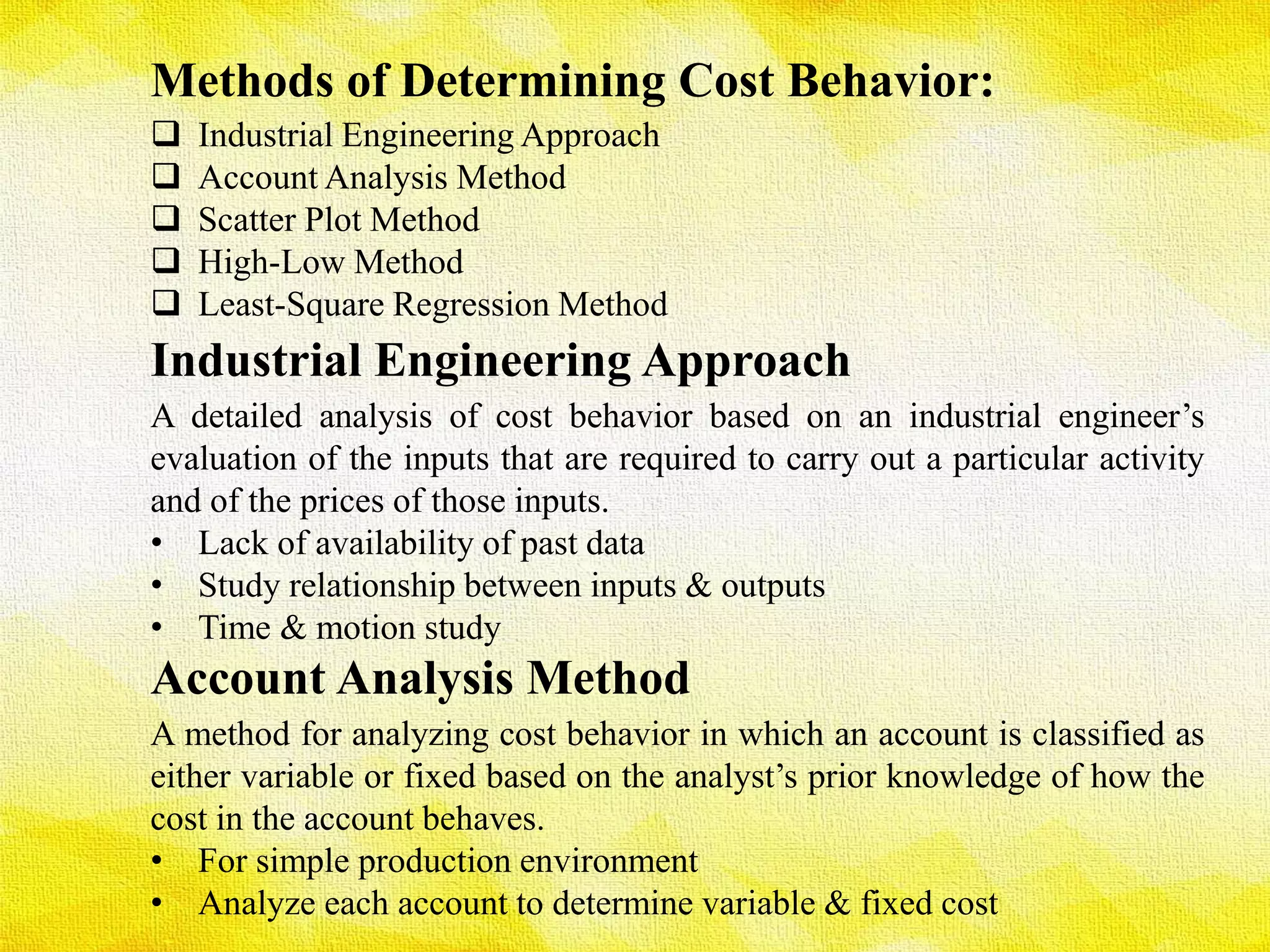
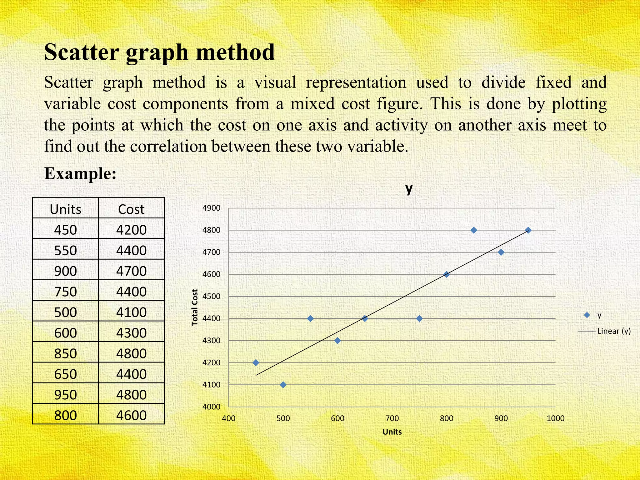
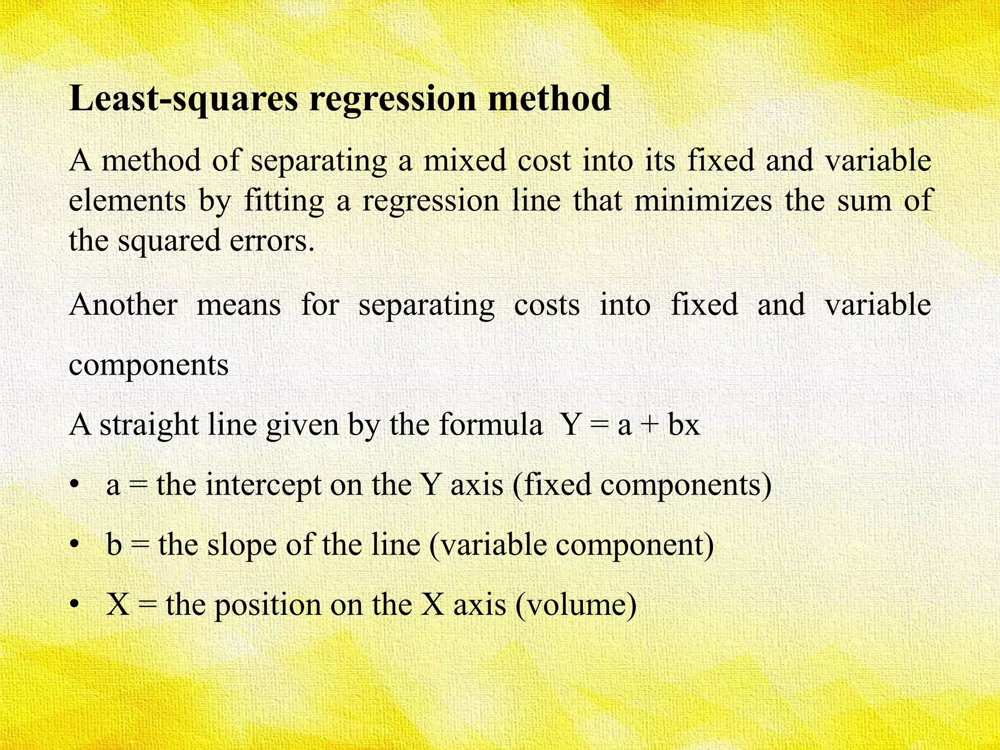
Presentation on
Methods of Determining Cost Behavior
Prepared by
md. Riduanul islam
Id no: r 202024
Methods of Determining Cost Behavior:
 Industrial Engineering Approach
 Account Analysis Method
 Scatter Plot Method
 High-Low Method
 Least-Square Regression Method
Industrial Engineering Approach
A detailed analysis of cost behavior based on an industrial engineer’s
evaluation of the inputs that are required to carry out a particular activity
and of the prices of those inputs.
• Lack of availability of past data
• Study relationship between inputs & outputs
• Time & motion study
Account Analysis Method
A method for analyzing cost behavior in which an account is classified as
either variable or fixed based on the analyst’s prior knowledge of how the
cost in the account behaves.
• For simple production environment
• Analyze each account to determine variable & fixed cost
4000
4100
4200
4300
4400
4500
4600
4700
4800
4900
400 500 600 700 800 900 1000
TotalCost
Units
y
y
Linear (y)
Units Cost
450 4200
550 4400
900 4700
750 4400
500 4100
600 4300
850 4800
650 4400
950 4800
800 4600
Scatter graph method
Scatter graph method is a visual representation used to divide fixed and
variable cost components from a mixed cost figure. This is done by plotting
the points at which the cost on one axis and activity on another axis meet to
find out the correlation between these two variable.
Example:
High-Low Method
The high-low method involves taking the highest level of activity
and the lowest level of activity and comparing the total costs at
each level.
• The highest and lowest levels of activity are identified
• The difference in cost between the points represents variable
cost associated with the change in activity
• A per unit variable cost can then be computed
• Finally, fixed cost can be calculated
The Equation: Y = a + bx
Y = 3660 + 1.2 x
Unit Cost
450 4200
550 4400
900 4700
750 4400
500 4100
600 4300
850 4800
650 4400
950 4800
800 4600
Variable Cost Per Unit
High Low Change VCPU
Cost 4800 4200 600
1.2
Unit 950 450 500
FC = TC - TVC
TC VCPU Volume TVC=(VCPU x Volume) FC
High 4800 1.2 950 1140 3660
Low 4200 1.2 450 540 3660
Example of High-Low method:
Least-squares regression method
A method of separating a mixed cost into its fixed and variable
elements by fitting a regression line that minimizes the sum of
the squared errors.
Another means for separating costs into fixed and variable
components
A straight line given by the formula Y = a + bx
• a = the intercept on the Y axis (fixed components)
• b = the slope of the line (variable component)
• X = the position on the X axis (volume)
X(Unit) Y(Cost) XY X²
450 4200 1890000 202500
550 4400 2420000 302500
900 4700 4230000 810000
750 4400 3300000 562500
500 4100 2050000 250000
600 4300 2580000 360000
850 4800 4080000 722500
650 4400 2860000 422500
950 4800 4560000 902500
800 4600 3680000 640000
ƩX ƩY ƩXY ƩX²
7000 44700 31650000 5175000
Unit Cost
450 4200
550 4400
900 4700
750 4400
500 4100
600 4300
850 4800
650 4400
950 4800
800 4600
= 1.3090909
= 1.31
= 3553.6364
= 3553.64
Here,
n = 10
The Equation: Y = a + bx
Y = 3553.64 + 1.31 x
Example of Least-squares regression method:
Thank you

Presentation on Methods of Determining Cost Behavior

  • 1.
    Presentation on Methods ofDetermining Cost Behavior Prepared by md. Riduanul islam Id no: r 202024
  • 2.
    Methods of DeterminingCost Behavior:  Industrial Engineering Approach  Account Analysis Method  Scatter Plot Method  High-Low Method  Least-Square Regression Method Industrial Engineering Approach A detailed analysis of cost behavior based on an industrial engineer’s evaluation of the inputs that are required to carry out a particular activity and of the prices of those inputs. • Lack of availability of past data • Study relationship between inputs & outputs • Time & motion study Account Analysis Method A method for analyzing cost behavior in which an account is classified as either variable or fixed based on the analyst’s prior knowledge of how the cost in the account behaves. • For simple production environment • Analyze each account to determine variable & fixed cost
  • 3.
    4000 4100 4200 4300 4400 4500 4600 4700 4800 4900 400 500 600700 800 900 1000 TotalCost Units y y Linear (y) Units Cost 450 4200 550 4400 900 4700 750 4400 500 4100 600 4300 850 4800 650 4400 950 4800 800 4600 Scatter graph method Scatter graph method is a visual representation used to divide fixed and variable cost components from a mixed cost figure. This is done by plotting the points at which the cost on one axis and activity on another axis meet to find out the correlation between these two variable. Example:
  • 4.
    High-Low Method The high-lowmethod involves taking the highest level of activity and the lowest level of activity and comparing the total costs at each level. • The highest and lowest levels of activity are identified • The difference in cost between the points represents variable cost associated with the change in activity • A per unit variable cost can then be computed • Finally, fixed cost can be calculated
  • 5.
    The Equation: Y= a + bx Y = 3660 + 1.2 x Unit Cost 450 4200 550 4400 900 4700 750 4400 500 4100 600 4300 850 4800 650 4400 950 4800 800 4600 Variable Cost Per Unit High Low Change VCPU Cost 4800 4200 600 1.2 Unit 950 450 500 FC = TC - TVC TC VCPU Volume TVC=(VCPU x Volume) FC High 4800 1.2 950 1140 3660 Low 4200 1.2 450 540 3660 Example of High-Low method:
  • 6.
    Least-squares regression method Amethod of separating a mixed cost into its fixed and variable elements by fitting a regression line that minimizes the sum of the squared errors. Another means for separating costs into fixed and variable components A straight line given by the formula Y = a + bx • a = the intercept on the Y axis (fixed components) • b = the slope of the line (variable component) • X = the position on the X axis (volume)
  • 7.
    X(Unit) Y(Cost) XYX² 450 4200 1890000 202500 550 4400 2420000 302500 900 4700 4230000 810000 750 4400 3300000 562500 500 4100 2050000 250000 600 4300 2580000 360000 850 4800 4080000 722500 650 4400 2860000 422500 950 4800 4560000 902500 800 4600 3680000 640000 ƩX ƩY ƩXY ƩX² 7000 44700 31650000 5175000 Unit Cost 450 4200 550 4400 900 4700 750 4400 500 4100 600 4300 850 4800 650 4400 950 4800 800 4600 = 1.3090909 = 1.31 = 3553.6364 = 3553.64 Here, n = 10 The Equation: Y = a + bx Y = 3553.64 + 1.31 x Example of Least-squares regression method:
  • 8.