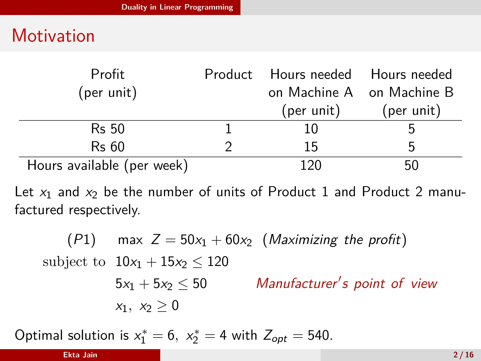
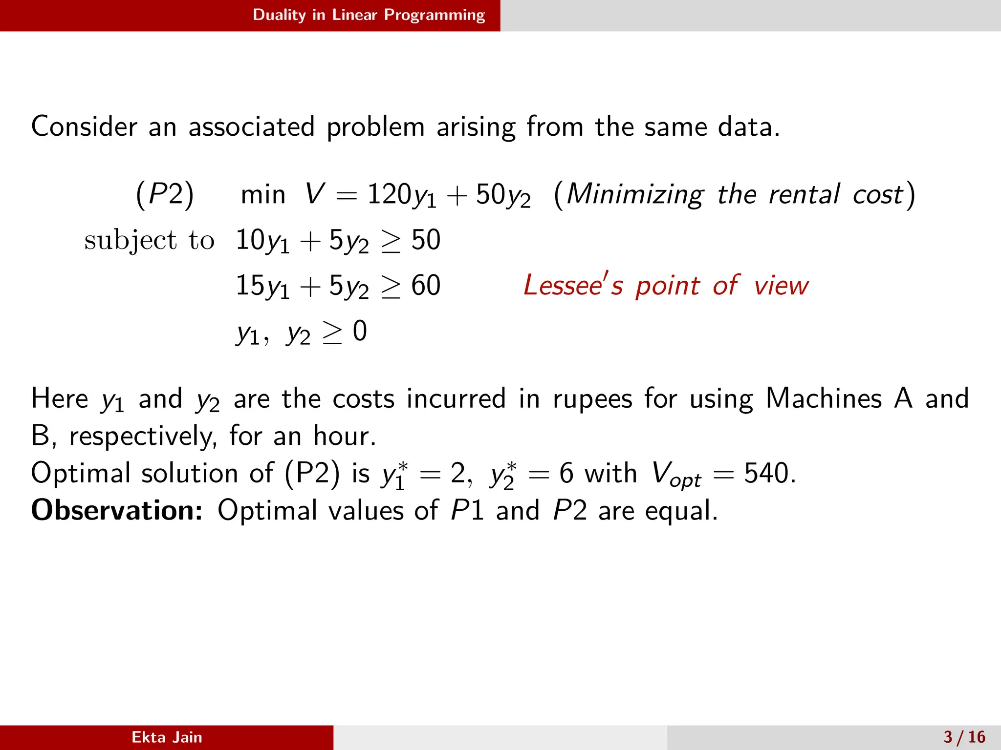
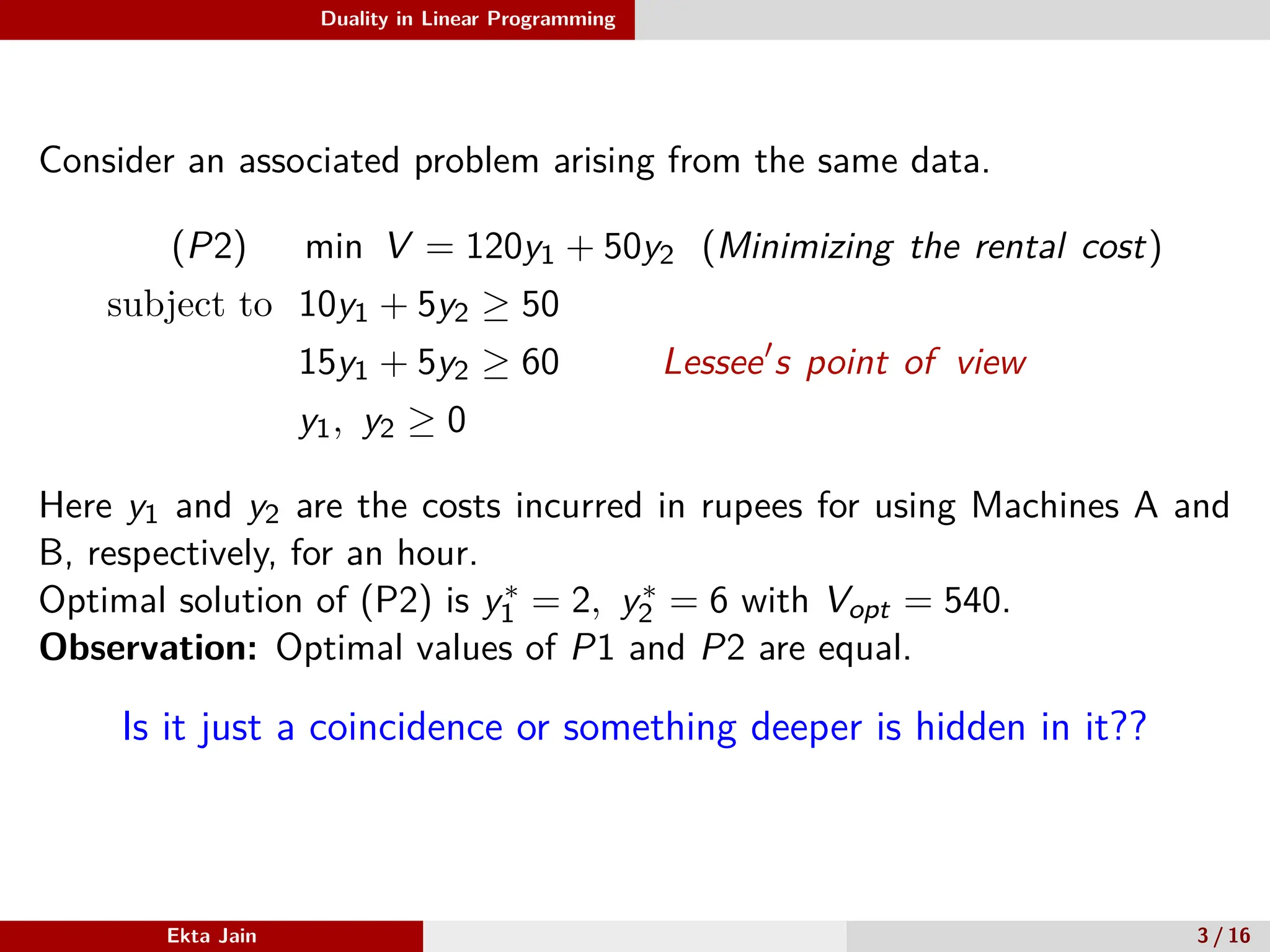
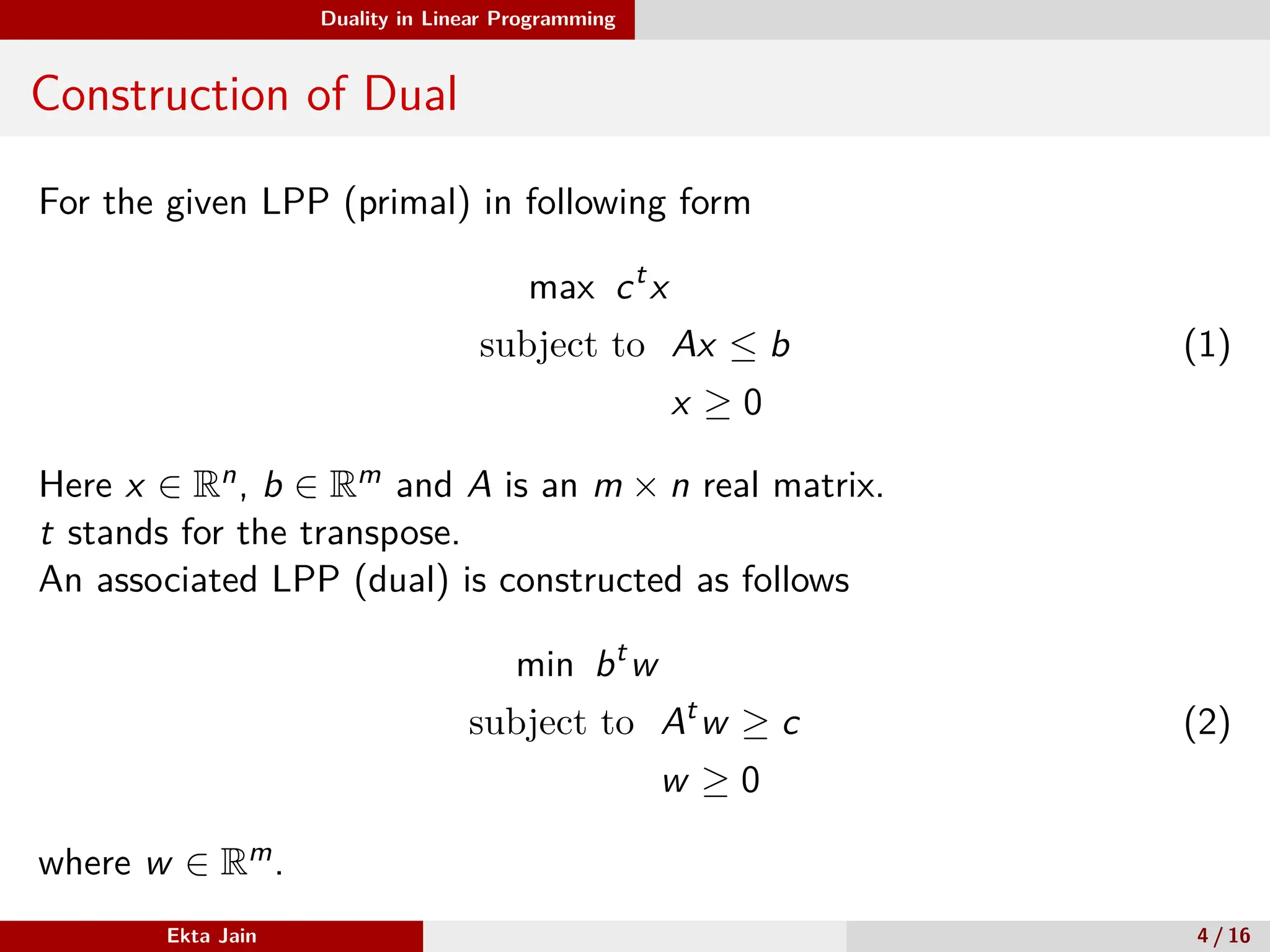
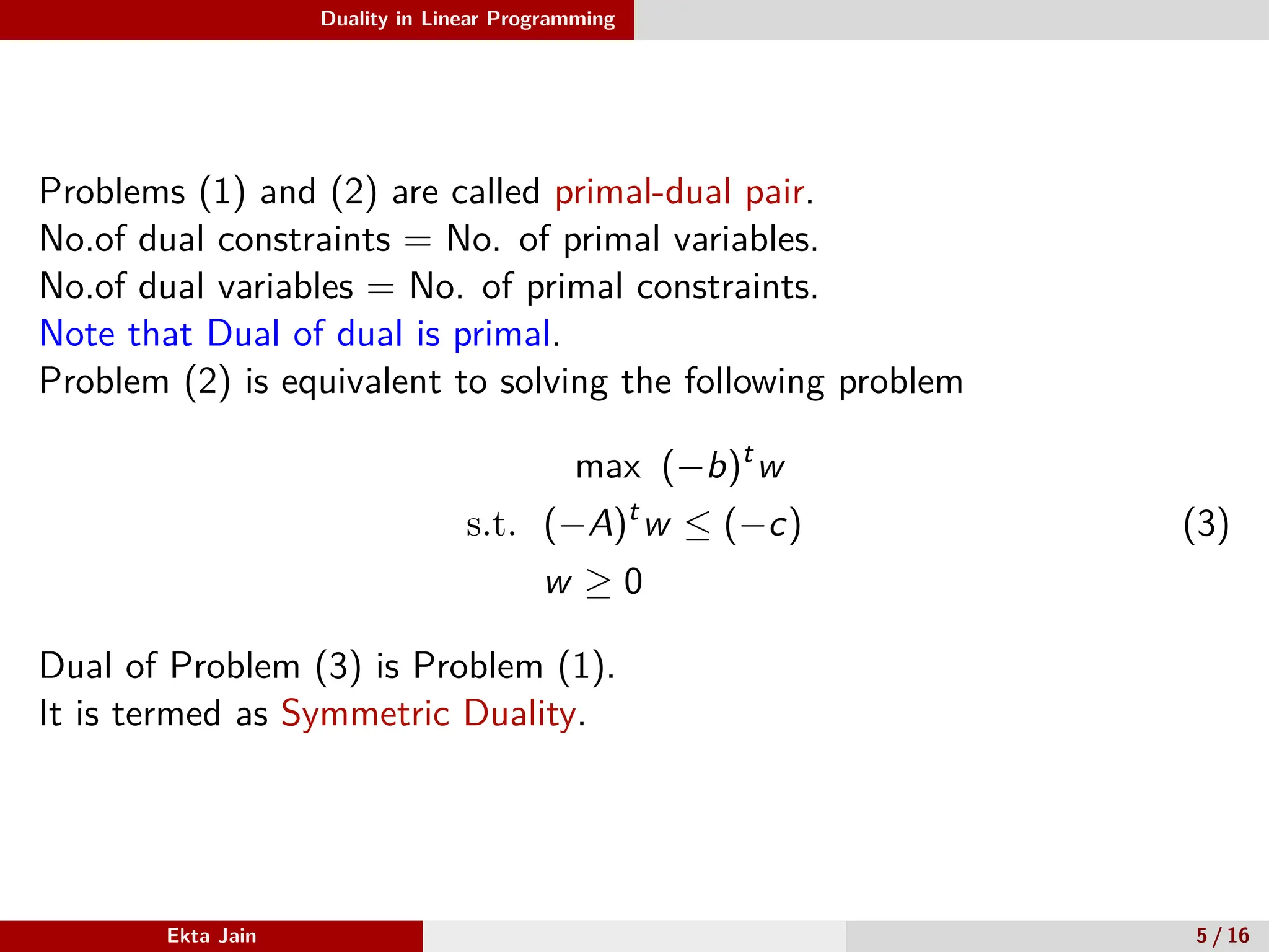
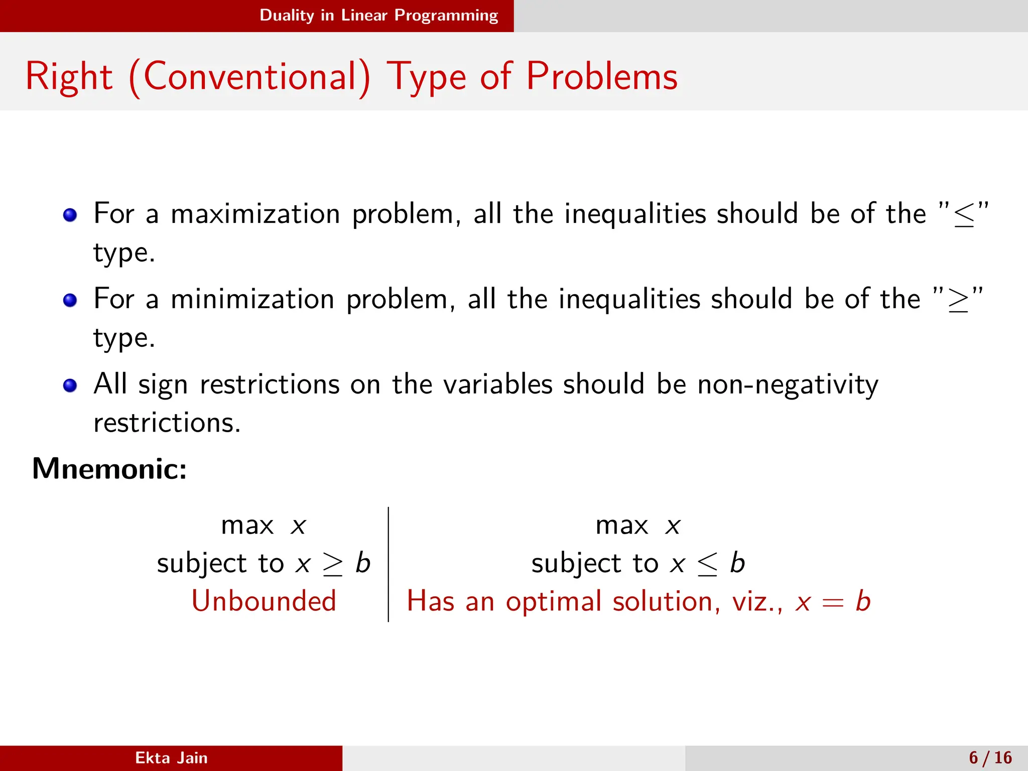
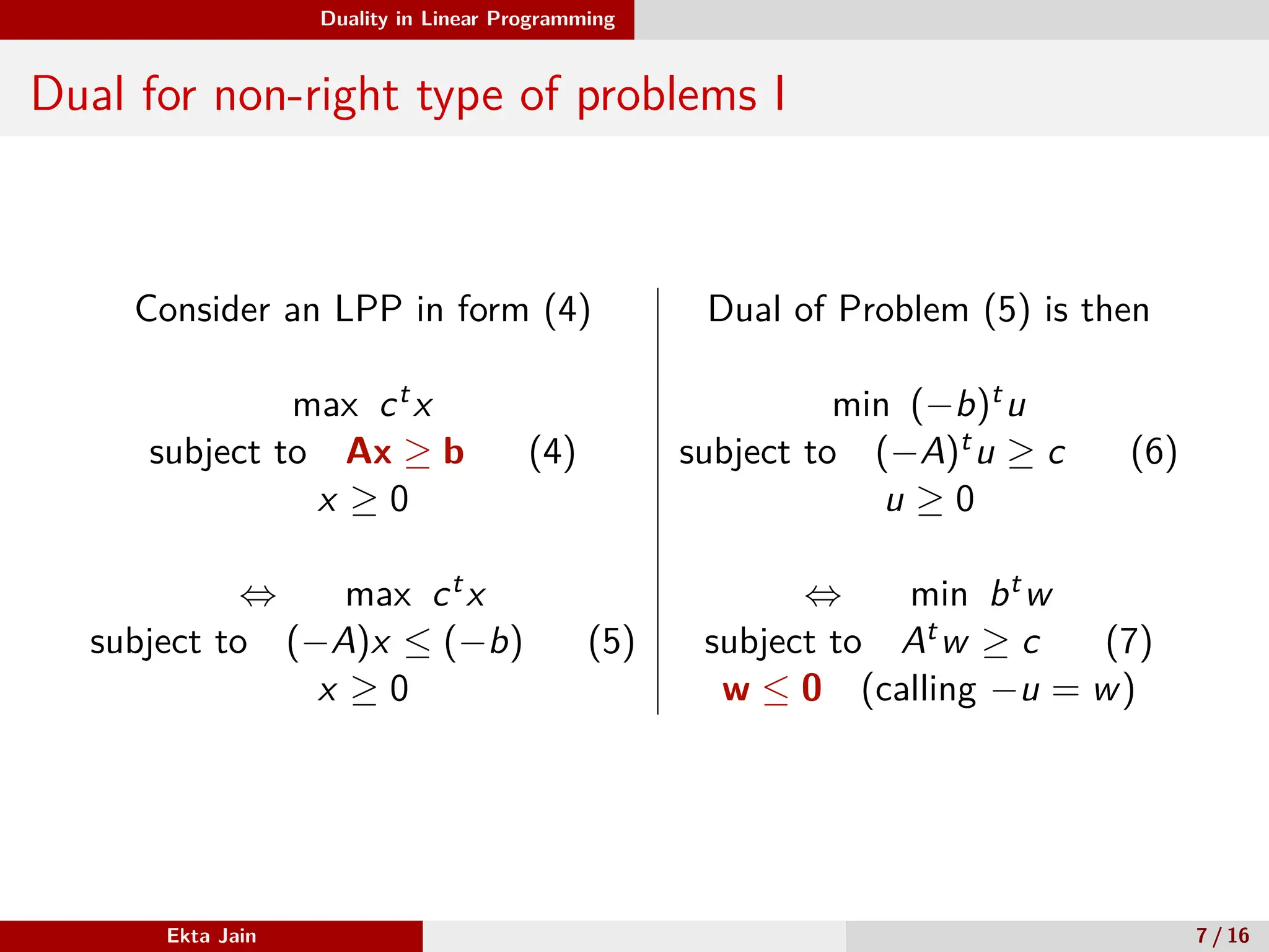
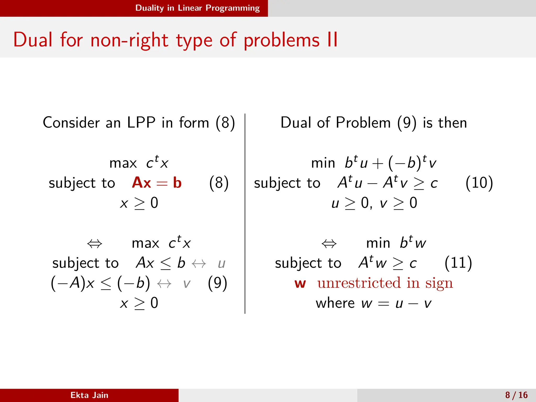
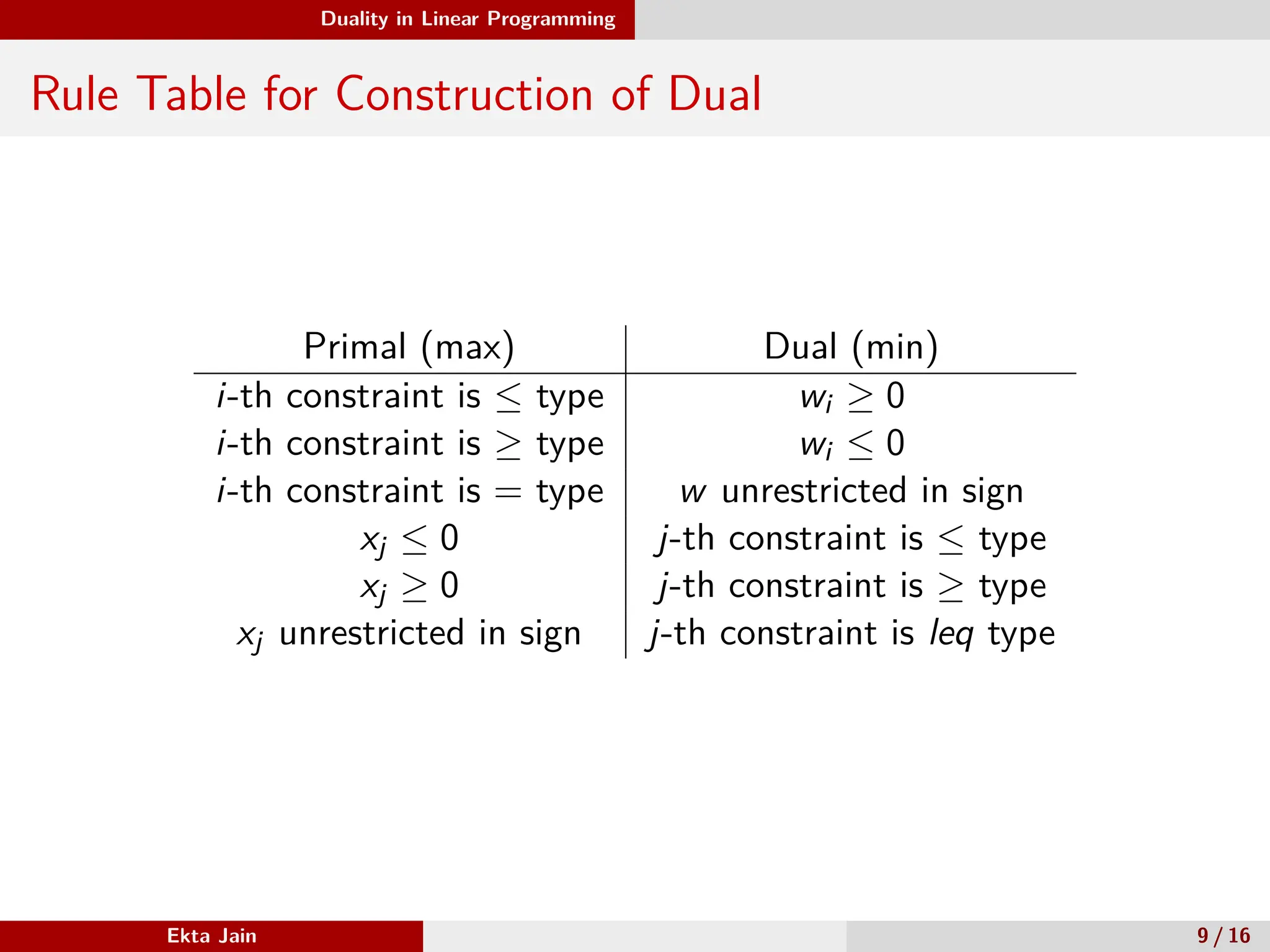
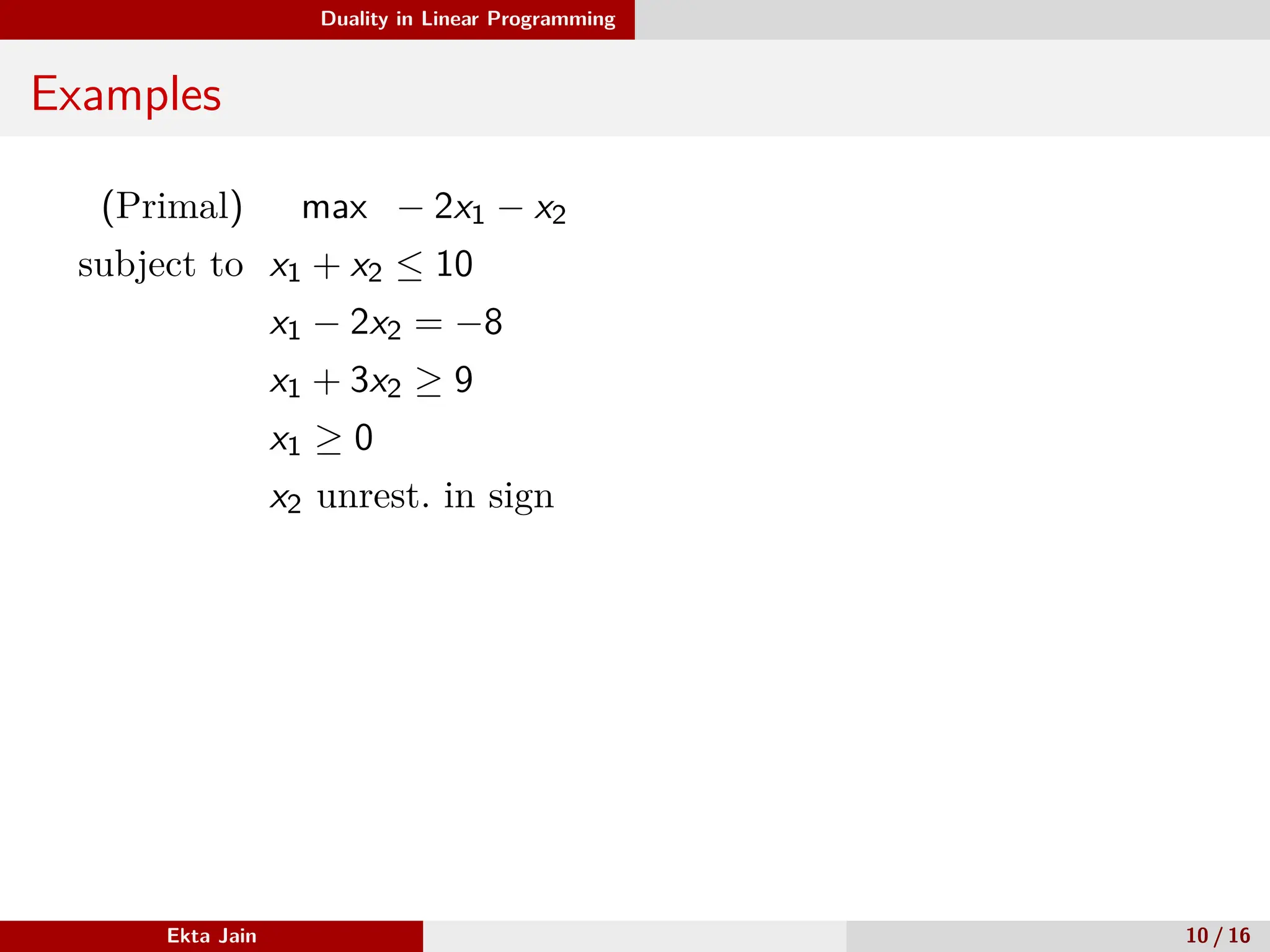
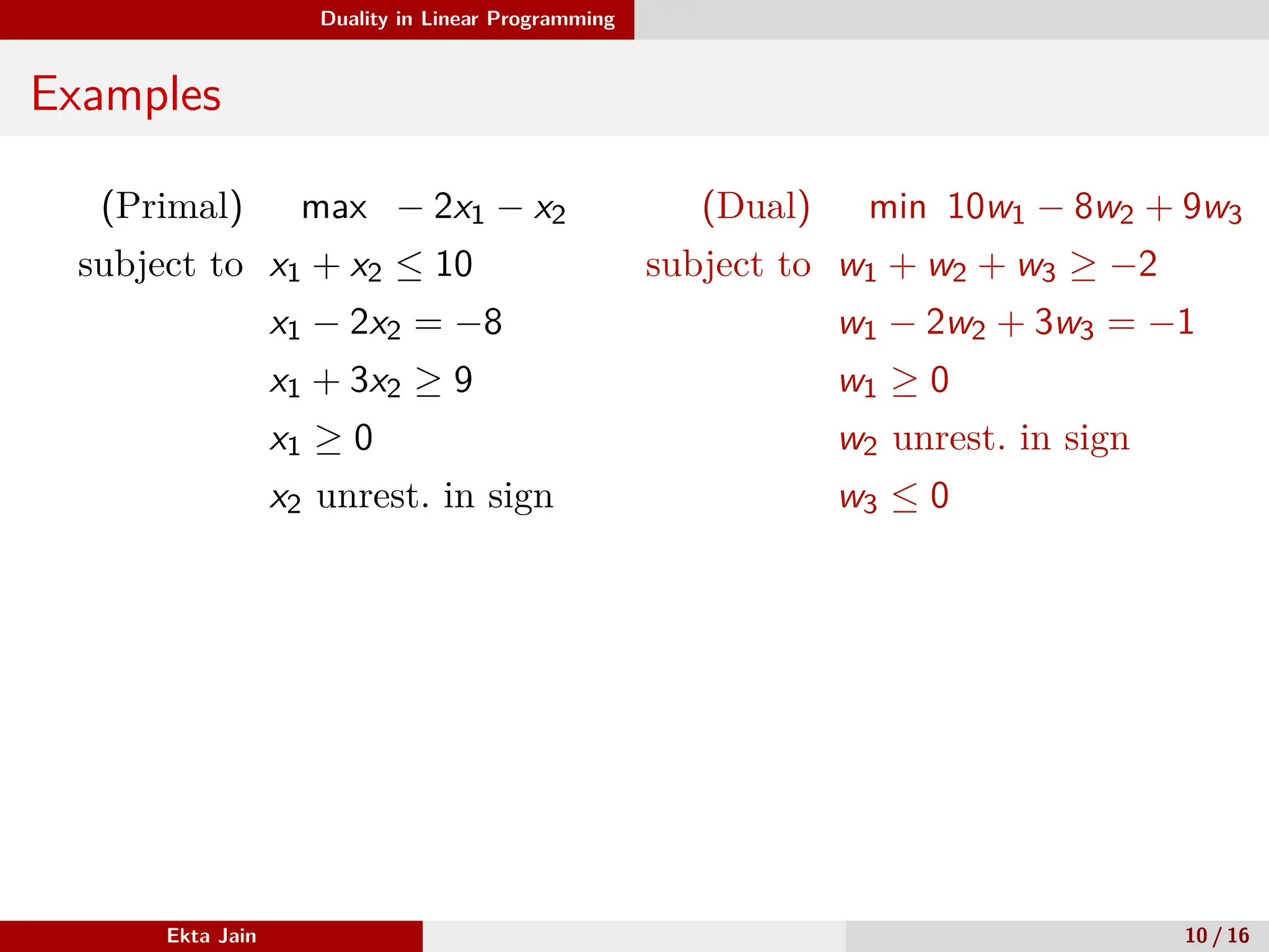
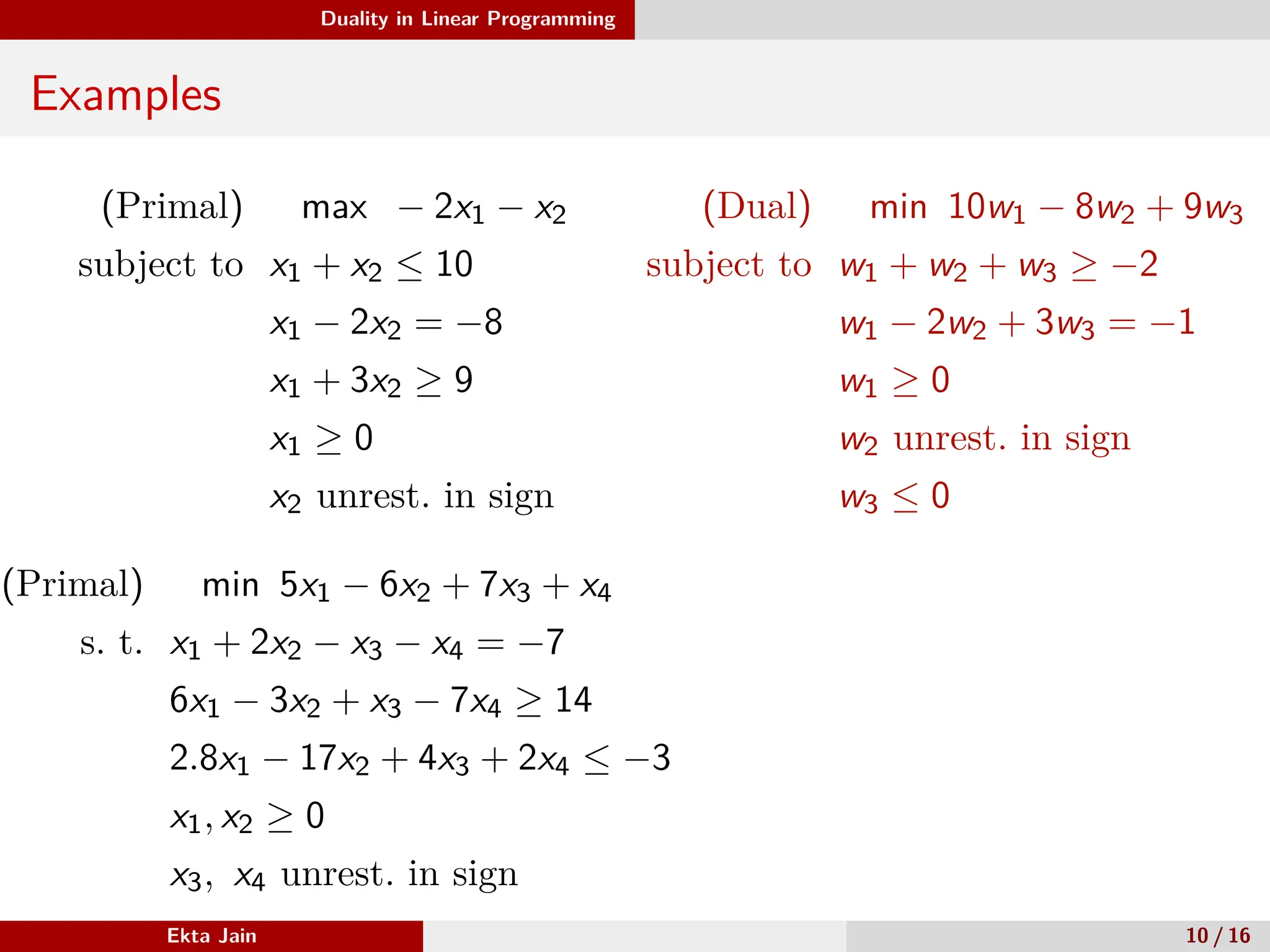
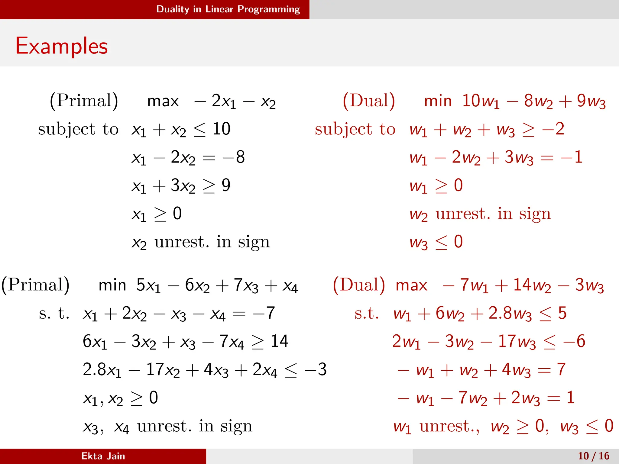
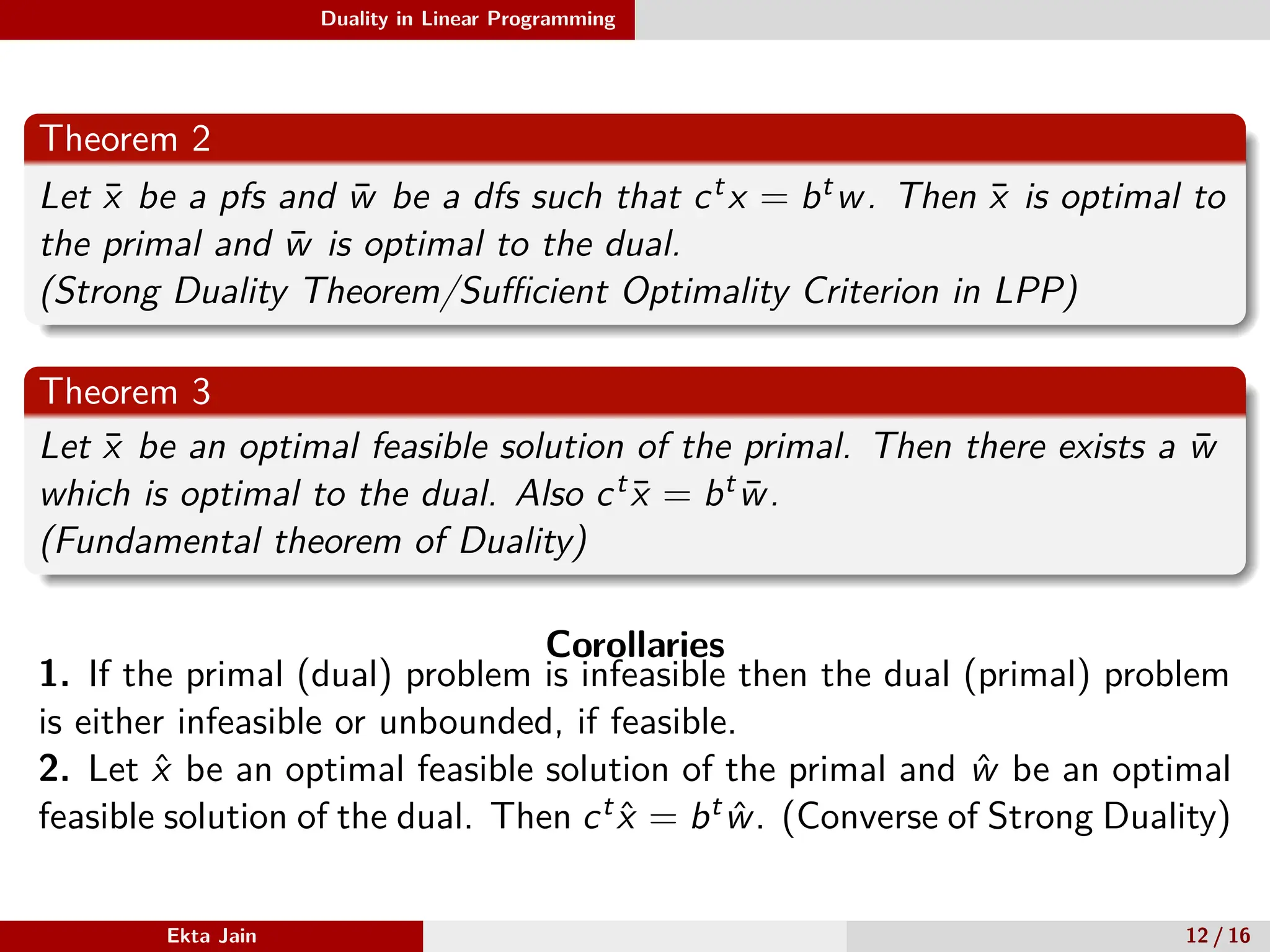
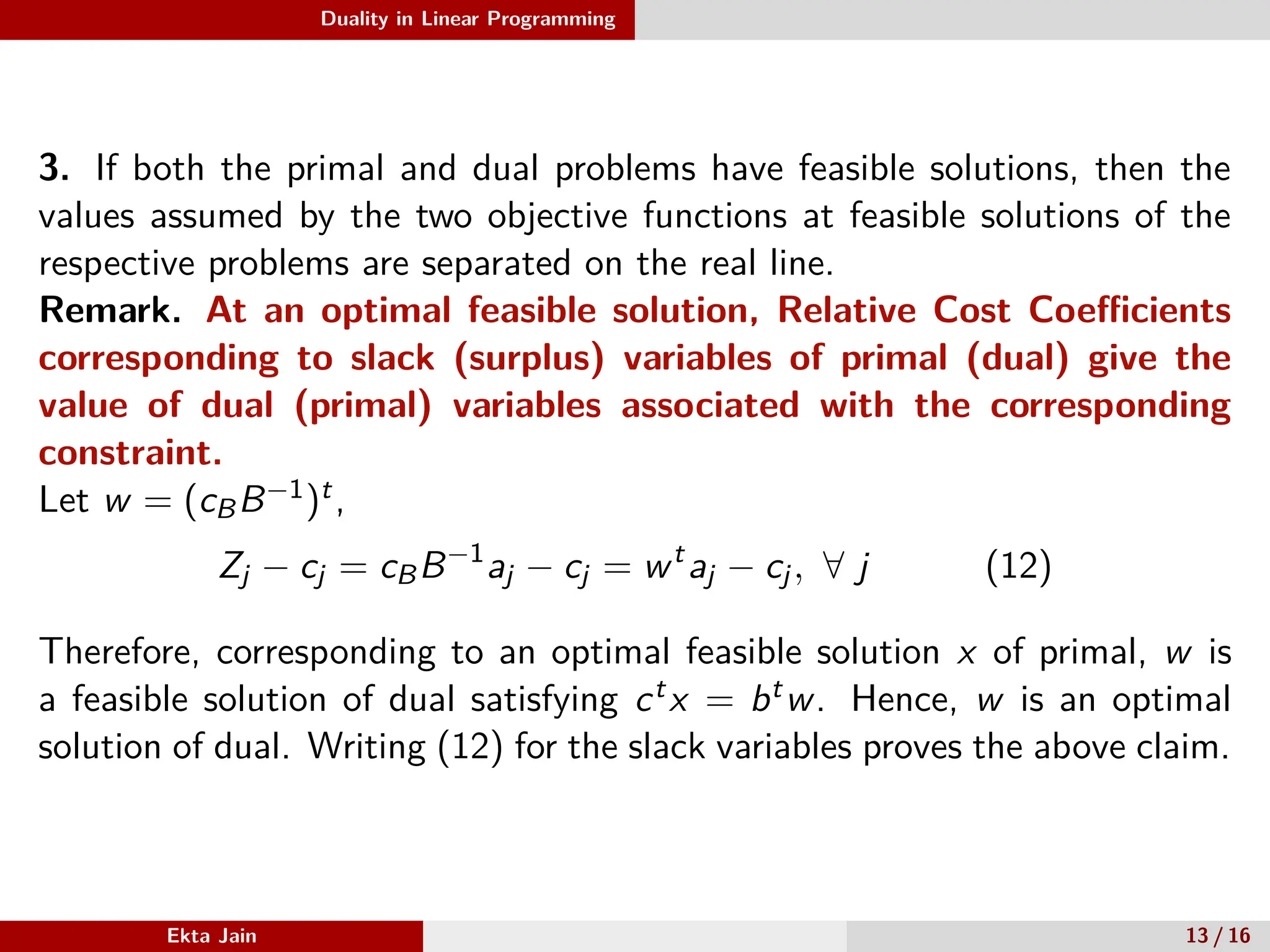
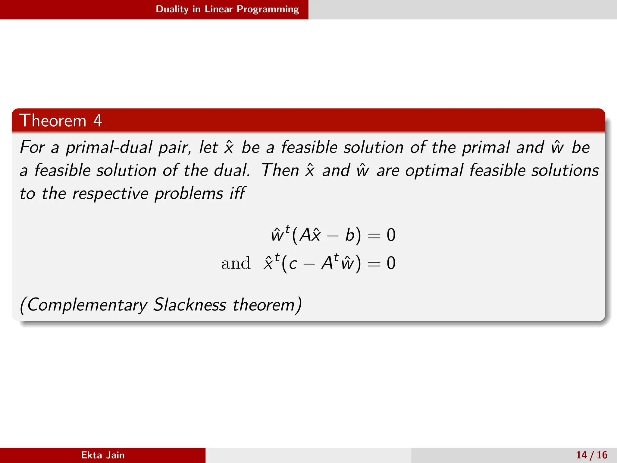
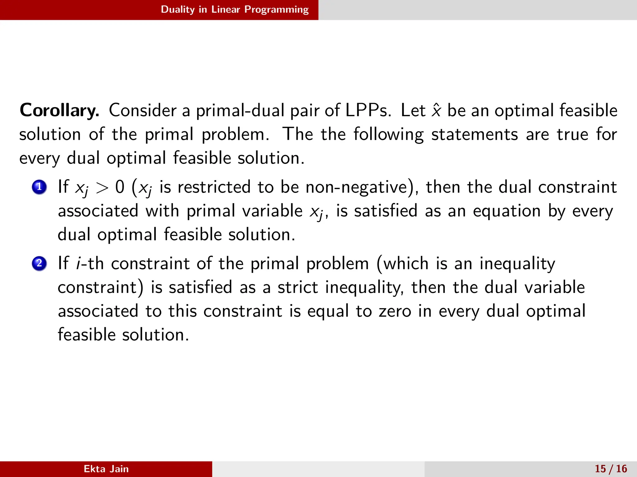
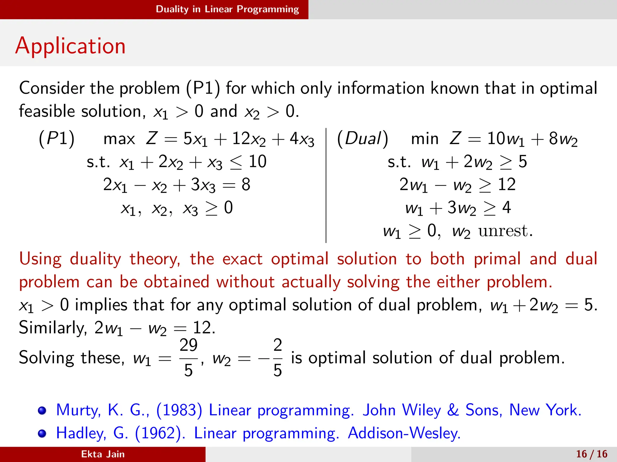
Duality in Linear Programming
Teaching Demonstration
Duality in Linear Programming
Ekta Jain 1 / 16
Duality in Linear Programming
Motivation
Profit Product Hours needed Hours needed
(per unit) on Machine A on Machine B
(per unit) (per unit)
Rs 50 1 10 5
Rs 60 2 15 5
Hours available (per week) 120 50
Let x1 and x2 be the number of units of Product 1 and Product 2 manu-
factured respectively.
(P1) max Z = 50x1 + 60x2 (Maximizing the profit)
subject to 10x1 + 15x2 ≤ 120
5x1 + 5x2 ≤ 50 Manufacturer′
s point of view
x1, x2 ≥ 0
Optimal solution is x∗
1 = 6, x∗
2 = 4 with Zopt = 540.
Ekta Jain 2 / 16
Duality in Linear Programming
Consider an associated problem arising from the same data.
(P2) min V = 120y1 + 50y2 (Minimizing the rental cost)
subject to 10y1 + 5y2 ≥ 50
15y1 + 5y2 ≥ 60 Lessee′
s point of view
y1, y2 ≥ 0
Here y1 and y2 are the costs incurred in rupees for using Machines A and
B, respectively, for an hour.
Optimal solution of (P2) is y∗
1 = 2, y∗
2 = 6 with Vopt = 540.
Observation: Optimal values of P1 and P2 are equal.
Ekta Jain 3 / 16
Duality in Linear Programming
Consider an associated problem arising from the same data.
(P2) min V = 120y1 + 50y2 (Minimizing the rental cost)
subject to 10y1 + 5y2 ≥ 50
15y1 + 5y2 ≥ 60 Lessee′
s point of view
y1, y2 ≥ 0
Here y1 and y2 are the costs incurred in rupees for using Machines A and
B, respectively, for an hour.
Optimal solution of (P2) is y∗
1 = 2, y∗
2 = 6 with Vopt = 540.
Observation: Optimal values of P1 and P2 are equal.
Is it just a coincidence or something deeper is hidden in it??
Ekta Jain 3 / 16
Duality in Linear Programming
Construction of Dual
For the given LPP (primal) in following form
max ct
x
subject to Ax ≤ b
x ≥ 0
(1)
Here x ∈ Rn, b ∈ Rm and A is an m × n real matrix.
t stands for the transpose.
An associated LPP (dual) is constructed as follows
min bt
w
subject to At
w ≥ c
w ≥ 0
(2)
where w ∈ Rm.
Ekta Jain 4 / 16
Duality in Linear Programming
Problems (1) and (2) are called primal-dual pair.
No.of dual constraints = No. of primal variables.
No.of dual variables = No. of primal constraints.
Note that Dual of dual is primal.
Problem (2) is equivalent to solving the following problem
max (−b)t
w
s.t. (−A)t
w ≤ (−c)
w ≥ 0
(3)
Dual of Problem (3) is Problem (1).
It is termed as Symmetric Duality.
Ekta Jain 5 / 16
Duality in Linear Programming
Right (Conventional) Type of Problems
For a maximization problem, all the inequalities should be of the ”≤”
type.
For a minimization problem, all the inequalities should be of the ”≥”
type.
All sign restrictions on the variables should be non-negativity
restrictions.
Mnemonic:
max x max x
subject to x ≥ b subject to x ≤ b
Unbounded Has an optimal solution, viz., x = b
Ekta Jain 6 / 16
Duality in Linear Programming
Dual for non-right type of problems I
Consider an LPP in form (4) Dual of Problem (5) is then
max ctx min (−b)tu
subject to Ax ≥ b (4) subject to (−A)tu ≥ c (6)
x ≥ 0 u ≥ 0
⇔ max ctx ⇔ min btw
subject to (−A)x ≤ (−b) (5) subject to Atw ≥ c (7)
x ≥ 0 w ≤ 0 (calling −u = w)
Ekta Jain 7 / 16
Duality in Linear Programming
Dual for non-right type of problems II
Consider an LPP in form (8) Dual of Problem (9) is then
max ctx min btu + (−b)tv
subject to Ax = b (8) subject to Atu − Atv ≥ c (10)
x ≥ 0 u ≥ 0, v ≥ 0
⇔ max ctx ⇔ min btw
subject to Ax ≤ b ↔ u subject to Atw ≥ c (11)
(−A)x ≤ (−b) ↔ v (9) w unrestricted in sign
x ≥ 0 where w = u − v
Ekta Jain 8 / 16
Duality in Linear Programming
Rule Table for Construction of Dual
Primal (max) Dual (min)
i-th constraint is ≤ type wi ≥ 0
i-th constraint is ≥ type wi ≤ 0
i-th constraint is = type w unrestricted in sign
xj ≤ 0 j-th constraint is ≤ type
xj ≥ 0 j-th constraint is ≥ type
xj unrestricted in sign j-th constraint is leq type
Ekta Jain 9 / 16
Duality in Linear Programming
Examples
(Primal) max − 2x1 − x2
subject to x1 + x2 ≤ 10
x1 − 2x2 = −8
x1 + 3x2 ≥ 9
x1 ≥ 0
x2 unrest. in sign
Ekta Jain 10 / 16
Duality in Linear Programming
Examples
(Primal) max − 2x1 − x2
subject to x1 + x2 ≤ 10
x1 − 2x2 = −8
x1 + 3x2 ≥ 9
x1 ≥ 0
x2 unrest. in sign
(Dual) min 10w1 − 8w2 + 9w3
subject to w1 + w2 + w3 ≥ −2
w1 − 2w2 + 3w3 = −1
w1 ≥ 0
w2 unrest. in sign
w3 ≤ 0
Ekta Jain 10 / 16
Duality in Linear Programming
Examples
(Primal) max − 2x1 − x2
subject to x1 + x2 ≤ 10
x1 − 2x2 = −8
x1 + 3x2 ≥ 9
x1 ≥ 0
x2 unrest. in sign
(Dual) min 10w1 − 8w2 + 9w3
subject to w1 + w2 + w3 ≥ −2
w1 − 2w2 + 3w3 = −1
w1 ≥ 0
w2 unrest. in sign
w3 ≤ 0
(Primal) min 5x1 − 6x2 + 7x3 + x4
s. t. x1 + 2x2 − x3 − x4 = −7
6x1 − 3x2 + x3 − 7x4 ≥ 14
2.8x1 − 17x2 + 4x3 + 2x4 ≤ −3
x1, x2 ≥ 0
x3, x4 unrest. in sign
(Dual) max − 7w1 + 14w2 − 3w3
s.t. w1 + 6w2 + 2.8w3 ≤ 5
2w1 − 3w2 − 17w3 ≤ −6
− w1 + w2 + 4w3 = 7
− w1 − 7w2 + 2w3 = 1
w1 unrest., w2 ≥ 0, w3 ≤ 0
Ekta Jain 10 / 16
Duality in Linear Programming
Duality Theorems
Referring Problem (1) as primal problem and Problem (2) as dual problem.
Theorem 1
For a primal-dual pair of LPPs, let ‘x’ be a primal feasible solution (pfs)
and ‘w’ a dual feasible solution (dfs), then
ct
x ≤ bt
w
(Weak Duality Theorem)
Corollaries
1 The primal objective value of any pfs is a lower bound to the minimum
value of the dual objective in dual problem. Similarly other case.
2 Primal (dual) problem unbounded implies the dual (primal) problem is
infeasible.
Ekta Jain 11 / 16
Duality in Linear Programming
Theorem 2
Let x̄ be a pfs and w̄ be a dfs such that ctx = btw. Then x̄ is optimal to
the primal and w̄ is optimal to the dual.
(Strong Duality Theorem/Sufficient Optimality Criterion in LPP)
Theorem 3
Let x̄ be an optimal feasible solution of the primal. Then there exists a w̄
which is optimal to the dual. Also ctx̄ = btw̄.
(Fundamental theorem of Duality)
Corollaries
1. If the primal (dual) problem is infeasible then the dual (primal) problem
is either infeasible or unbounded, if feasible.
2. Let x̂ be an optimal feasible solution of the primal and ŵ be an optimal
feasible solution of the dual. Then ctx̂ = btŵ. (Converse of Strong Duality)
Ekta Jain 12 / 16
Duality in Linear Programming
3. If both the primal and dual problems have feasible solutions, then the
values assumed by the two objective functions at feasible solutions of the
respective problems are separated on the real line.
Ekta Jain 13 / 16
Duality in Linear Programming
3. If both the primal and dual problems have feasible solutions, then the
values assumed by the two objective functions at feasible solutions of the
respective problems are separated on the real line.
Remark. At an optimal feasible solution, Relative Cost Coefficients
corresponding to slack (surplus) variables of primal (dual) give the
value of dual (primal) variables associated with the corresponding
constraint.
Let w = (cBB−1)t,
Zj − cj = cBB−1
aj − cj = wt
aj − cj, ∀ j (12)
Therefore, corresponding to an optimal feasible solution x of primal, w is
a feasible solution of dual satisfying ctx = btw. Hence, w is an optimal
solution of dual. Writing (12) for the slack variables proves the above claim.
Ekta Jain 13 / 16
Duality in Linear Programming
Theorem 4
For a primal-dual pair, let x̂ be a feasible solution of the primal and ŵ be
a feasible solution of the dual. Then x̂ and ŵ are optimal feasible solutions
to the respective problems iff
ŵt
(Ax̂ − b) = 0
and x̂t
(c − At
ŵ) = 0
(Complementary Slackness theorem)
Ekta Jain 14 / 16
Duality in Linear Programming
Corollary. Consider a primal-dual pair of LPPs. Let x̂ be an optimal feasible
solution of the primal problem. The the following statements are true for
every dual optimal feasible solution.
1 If xj > 0 (xj is restricted to be non-negative), then the dual constraint
associated with primal variable xj, is satisfied as an equation by every
dual optimal feasible solution.
2 If i-th constraint of the primal problem (which is an inequality
constraint) is satisfied as a strict inequality, then the dual variable
associated to this constraint is equal to zero in every dual optimal
feasible solution.
Ekta Jain 15 / 16
Duality in Linear Programming
Application
Consider the problem (P1) for which only information known that in optimal
feasible solution, x1 > 0 and x2 > 0.
(P1) max Z = 5x1 + 12x2 + 4x3 (Dual) min Z = 10w1 + 8w2
s.t. x1 + 2x2 + x3 ≤ 10 s.t. w1 + 2w2 ≥ 5
2x1 − x2 + 3x3 = 8 2w1 − w2 ≥ 12
x1, x2, x3 ≥ 0 w1 + 3w2 ≥ 4
w1 ≥ 0, w2 unrest.
Using duality theory, the exact optimal solution to both primal and dual
problem can be obtained without actually solving the either problem.
x1 > 0 implies that for any optimal solution of dual problem, w1 +2w2 = 5.
Similarly, 2w1 − w2 = 12.
Solving these, w1 =
29
5
, w2 = −
2
5
is optimal solution of dual problem.
Murty, K. G., (1983) Linear programming. John Wiley & Sons, New York.
Hadley, G. (1962). Linear programming. Addison-Wesley.
Ekta Jain 16 / 16

presentation on Duality theory in operations research

  • 1.
    Duality in LinearProgramming Teaching Demonstration Duality in Linear Programming Ekta Jain 1 / 16
  • 2.
    Duality in LinearProgramming Motivation Profit Product Hours needed Hours needed (per unit) on Machine A on Machine B (per unit) (per unit) Rs 50 1 10 5 Rs 60 2 15 5 Hours available (per week) 120 50 Let x1 and x2 be the number of units of Product 1 and Product 2 manu- factured respectively. (P1) max Z = 50x1 + 60x2 (Maximizing the profit) subject to 10x1 + 15x2 ≤ 120 5x1 + 5x2 ≤ 50 Manufacturer′ s point of view x1, x2 ≥ 0 Optimal solution is x∗ 1 = 6, x∗ 2 = 4 with Zopt = 540. Ekta Jain 2 / 16
  • 3.
    Duality in LinearProgramming Consider an associated problem arising from the same data. (P2) min V = 120y1 + 50y2 (Minimizing the rental cost) subject to 10y1 + 5y2 ≥ 50 15y1 + 5y2 ≥ 60 Lessee′ s point of view y1, y2 ≥ 0 Here y1 and y2 are the costs incurred in rupees for using Machines A and B, respectively, for an hour. Optimal solution of (P2) is y∗ 1 = 2, y∗ 2 = 6 with Vopt = 540. Observation: Optimal values of P1 and P2 are equal. Ekta Jain 3 / 16
  • 4.
    Duality in LinearProgramming Consider an associated problem arising from the same data. (P2) min V = 120y1 + 50y2 (Minimizing the rental cost) subject to 10y1 + 5y2 ≥ 50 15y1 + 5y2 ≥ 60 Lessee′ s point of view y1, y2 ≥ 0 Here y1 and y2 are the costs incurred in rupees for using Machines A and B, respectively, for an hour. Optimal solution of (P2) is y∗ 1 = 2, y∗ 2 = 6 with Vopt = 540. Observation: Optimal values of P1 and P2 are equal. Is it just a coincidence or something deeper is hidden in it?? Ekta Jain 3 / 16
  • 5.
    Duality in LinearProgramming Construction of Dual For the given LPP (primal) in following form max ct x subject to Ax ≤ b x ≥ 0 (1) Here x ∈ Rn, b ∈ Rm and A is an m × n real matrix. t stands for the transpose. An associated LPP (dual) is constructed as follows min bt w subject to At w ≥ c w ≥ 0 (2) where w ∈ Rm. Ekta Jain 4 / 16
  • 6.
    Duality in LinearProgramming Problems (1) and (2) are called primal-dual pair. No.of dual constraints = No. of primal variables. No.of dual variables = No. of primal constraints. Note that Dual of dual is primal. Problem (2) is equivalent to solving the following problem max (−b)t w s.t. (−A)t w ≤ (−c) w ≥ 0 (3) Dual of Problem (3) is Problem (1). It is termed as Symmetric Duality. Ekta Jain 5 / 16
  • 7.
    Duality in LinearProgramming Right (Conventional) Type of Problems For a maximization problem, all the inequalities should be of the ”≤” type. For a minimization problem, all the inequalities should be of the ”≥” type. All sign restrictions on the variables should be non-negativity restrictions. Mnemonic: max x max x subject to x ≥ b subject to x ≤ b Unbounded Has an optimal solution, viz., x = b Ekta Jain 6 / 16
  • 8.
    Duality in LinearProgramming Dual for non-right type of problems I Consider an LPP in form (4) Dual of Problem (5) is then max ctx min (−b)tu subject to Ax ≥ b (4) subject to (−A)tu ≥ c (6) x ≥ 0 u ≥ 0 ⇔ max ctx ⇔ min btw subject to (−A)x ≤ (−b) (5) subject to Atw ≥ c (7) x ≥ 0 w ≤ 0 (calling −u = w) Ekta Jain 7 / 16
  • 9.
    Duality in LinearProgramming Dual for non-right type of problems II Consider an LPP in form (8) Dual of Problem (9) is then max ctx min btu + (−b)tv subject to Ax = b (8) subject to Atu − Atv ≥ c (10) x ≥ 0 u ≥ 0, v ≥ 0 ⇔ max ctx ⇔ min btw subject to Ax ≤ b ↔ u subject to Atw ≥ c (11) (−A)x ≤ (−b) ↔ v (9) w unrestricted in sign x ≥ 0 where w = u − v Ekta Jain 8 / 16
  • 10.
    Duality in LinearProgramming Rule Table for Construction of Dual Primal (max) Dual (min) i-th constraint is ≤ type wi ≥ 0 i-th constraint is ≥ type wi ≤ 0 i-th constraint is = type w unrestricted in sign xj ≤ 0 j-th constraint is ≤ type xj ≥ 0 j-th constraint is ≥ type xj unrestricted in sign j-th constraint is leq type Ekta Jain 9 / 16
  • 11.
    Duality in LinearProgramming Examples (Primal) max − 2x1 − x2 subject to x1 + x2 ≤ 10 x1 − 2x2 = −8 x1 + 3x2 ≥ 9 x1 ≥ 0 x2 unrest. in sign Ekta Jain 10 / 16
  • 12.
    Duality in LinearProgramming Examples (Primal) max − 2x1 − x2 subject to x1 + x2 ≤ 10 x1 − 2x2 = −8 x1 + 3x2 ≥ 9 x1 ≥ 0 x2 unrest. in sign (Dual) min 10w1 − 8w2 + 9w3 subject to w1 + w2 + w3 ≥ −2 w1 − 2w2 + 3w3 = −1 w1 ≥ 0 w2 unrest. in sign w3 ≤ 0 Ekta Jain 10 / 16
  • 13.
    Duality in LinearProgramming Examples (Primal) max − 2x1 − x2 subject to x1 + x2 ≤ 10 x1 − 2x2 = −8 x1 + 3x2 ≥ 9 x1 ≥ 0 x2 unrest. in sign (Dual) min 10w1 − 8w2 + 9w3 subject to w1 + w2 + w3 ≥ −2 w1 − 2w2 + 3w3 = −1 w1 ≥ 0 w2 unrest. in sign w3 ≤ 0 (Primal) min 5x1 − 6x2 + 7x3 + x4 s. t. x1 + 2x2 − x3 − x4 = −7 6x1 − 3x2 + x3 − 7x4 ≥ 14 2.8x1 − 17x2 + 4x3 + 2x4 ≤ −3 x1, x2 ≥ 0 x3, x4 unrest. in sign Ekta Jain 10 / 16
  • 14.
    Duality in LinearProgramming Examples (Primal) max − 2x1 − x2 subject to x1 + x2 ≤ 10 x1 − 2x2 = −8 x1 + 3x2 ≥ 9 x1 ≥ 0 x2 unrest. in sign (Dual) min 10w1 − 8w2 + 9w3 subject to w1 + w2 + w3 ≥ −2 w1 − 2w2 + 3w3 = −1 w1 ≥ 0 w2 unrest. in sign w3 ≤ 0 (Primal) min 5x1 − 6x2 + 7x3 + x4 s. t. x1 + 2x2 − x3 − x4 = −7 6x1 − 3x2 + x3 − 7x4 ≥ 14 2.8x1 − 17x2 + 4x3 + 2x4 ≤ −3 x1, x2 ≥ 0 x3, x4 unrest. in sign (Dual) max − 7w1 + 14w2 − 3w3 s.t. w1 + 6w2 + 2.8w3 ≤ 5 2w1 − 3w2 − 17w3 ≤ −6 − w1 + w2 + 4w3 = 7 − w1 − 7w2 + 2w3 = 1 w1 unrest., w2 ≥ 0, w3 ≤ 0 Ekta Jain 10 / 16
  • 15.
    Duality in LinearProgramming Duality Theorems Referring Problem (1) as primal problem and Problem (2) as dual problem. Theorem 1 For a primal-dual pair of LPPs, let ‘x’ be a primal feasible solution (pfs) and ‘w’ a dual feasible solution (dfs), then ct x ≤ bt w (Weak Duality Theorem) Corollaries 1 The primal objective value of any pfs is a lower bound to the minimum value of the dual objective in dual problem. Similarly other case. 2 Primal (dual) problem unbounded implies the dual (primal) problem is infeasible. Ekta Jain 11 / 16
  • 16.
    Duality in LinearProgramming Theorem 2 Let x̄ be a pfs and w̄ be a dfs such that ctx = btw. Then x̄ is optimal to the primal and w̄ is optimal to the dual. (Strong Duality Theorem/Sufficient Optimality Criterion in LPP) Theorem 3 Let x̄ be an optimal feasible solution of the primal. Then there exists a w̄ which is optimal to the dual. Also ctx̄ = btw̄. (Fundamental theorem of Duality) Corollaries 1. If the primal (dual) problem is infeasible then the dual (primal) problem is either infeasible or unbounded, if feasible. 2. Let x̂ be an optimal feasible solution of the primal and ŵ be an optimal feasible solution of the dual. Then ctx̂ = btŵ. (Converse of Strong Duality) Ekta Jain 12 / 16
  • 17.
    Duality in LinearProgramming 3. If both the primal and dual problems have feasible solutions, then the values assumed by the two objective functions at feasible solutions of the respective problems are separated on the real line. Ekta Jain 13 / 16
  • 18.
    Duality in LinearProgramming 3. If both the primal and dual problems have feasible solutions, then the values assumed by the two objective functions at feasible solutions of the respective problems are separated on the real line. Remark. At an optimal feasible solution, Relative Cost Coefficients corresponding to slack (surplus) variables of primal (dual) give the value of dual (primal) variables associated with the corresponding constraint. Let w = (cBB−1)t, Zj − cj = cBB−1 aj − cj = wt aj − cj, ∀ j (12) Therefore, corresponding to an optimal feasible solution x of primal, w is a feasible solution of dual satisfying ctx = btw. Hence, w is an optimal solution of dual. Writing (12) for the slack variables proves the above claim. Ekta Jain 13 / 16
  • 19.
    Duality in LinearProgramming Theorem 4 For a primal-dual pair, let x̂ be a feasible solution of the primal and ŵ be a feasible solution of the dual. Then x̂ and ŵ are optimal feasible solutions to the respective problems iff ŵt (Ax̂ − b) = 0 and x̂t (c − At ŵ) = 0 (Complementary Slackness theorem) Ekta Jain 14 / 16
  • 20.
    Duality in LinearProgramming Corollary. Consider a primal-dual pair of LPPs. Let x̂ be an optimal feasible solution of the primal problem. The the following statements are true for every dual optimal feasible solution. 1 If xj > 0 (xj is restricted to be non-negative), then the dual constraint associated with primal variable xj, is satisfied as an equation by every dual optimal feasible solution. 2 If i-th constraint of the primal problem (which is an inequality constraint) is satisfied as a strict inequality, then the dual variable associated to this constraint is equal to zero in every dual optimal feasible solution. Ekta Jain 15 / 16
  • 21.
    Duality in LinearProgramming Application Consider the problem (P1) for which only information known that in optimal feasible solution, x1 > 0 and x2 > 0. (P1) max Z = 5x1 + 12x2 + 4x3 (Dual) min Z = 10w1 + 8w2 s.t. x1 + 2x2 + x3 ≤ 10 s.t. w1 + 2w2 ≥ 5 2x1 − x2 + 3x3 = 8 2w1 − w2 ≥ 12 x1, x2, x3 ≥ 0 w1 + 3w2 ≥ 4 w1 ≥ 0, w2 unrest. Using duality theory, the exact optimal solution to both primal and dual problem can be obtained without actually solving the either problem. x1 > 0 implies that for any optimal solution of dual problem, w1 +2w2 = 5. Similarly, 2w1 − w2 = 12. Solving these, w1 = 29 5 , w2 = − 2 5 is optimal solution of dual problem. Murty, K. G., (1983) Linear programming. John Wiley & Sons, New York. Hadley, G. (1962). Linear programming. Addison-Wesley. Ekta Jain 16 / 16