The document discusses methods for measuring star-formation rates (SFRs) in galaxies, presenting both historical context and various diagnostic techniques along the Hubble sequence. It details specific SFR measurement approaches, including continuum luminosity, UV luminosity, and recombination lines, while highlighting their advantages and limitations. The review emphasizes the complexities involved in calibrating SFRs quantitatively due to various dependencies on internal factors within galaxies.

1. Star Formation In Galaxies Along The Hubble
Sequence
Robert C. Kennicut, Jr.
(Annu. Rev. Astron. Astrophys. 1998. 36:189-231)
Christian Herenz
Extragalactic Science Club 2011
March 7th, 2012

2. Citations from ADS

3. The Author
Robert C. Kennicut, Jr.
Foto Source: http://www.flickr.com/photos/swilliams2001/4029565601/

4. Overview
Review is basically 2 Parts:
Diagnostic methods used to measure star-formation rates
(SFRs) in galaxies.
Systematics of SFRs along the Hubble Sequence.
This talk focuses on the first part, which is not merely a
summary, but
“... a self-consistent set of SFR calibrations is presented as an
aid to workers in the field.”
(from the Abstract)

5. Outline of this Talk
Historical Overview of SFR Measurements
SFR from Evolutionary Synthesis
SFR Diagnostics
1. Continuum Luminosity - Color Scaling Relation
2. UV Continuum Luminosity
3. H Recombination Lines
4. Forbidden Lines
5. FIR Continuum Emission
Summary

6. Historical Overview of SFR Measurements
Late 1960s: First quantitative SFRs from evolutionary
synthesis models (e.g. Beatrice Tinsley 1968 - Galaxy
Colors)
1970s-80s: Development of precise direct SFR calibrators.
emission-line fluxes
(near) UV continuum
IR continuum
Application to large galaxy samples. Interpretation in terms
of evolutionary properties.
1990s - present: Detection of star-forming galaxies at
high-z. Trace evolution of SFR density with look-back time
(e.g. Madau plot)

7. SFRs from Evolutionary Synthesis
Individual stars in galaxies typically unresolved
−→ SFRs derive from integrated light (Colors, UV, IR,
recombination lines).
Basis of all calibrators: Evolutionary Synthesis Models
(ESM)
Grid of stellar evolution tracks ˆ= T (t) & Lbol.
(t) for various
M .
Stellar atmosphere modells or spectral libraries: T (t) &
Lbol.
→ broadband colors or spectra (ˆ=Templates(t))
weighed by IMF Templates(t) = Luminosity, Color (and
spectrum) for single age population
For different SFH: Use linear-combination of single age
pops.
4 free parameters (at least): age, metalicity /
metal-abundance, IMF, SFH (constant / e−τ ...)
Synthesis modells can be downloaded / generated online
(e.g. GALEXV - Bruzal & Charlot)

8. SFR Diagnostic I. – Continuum Luminosity - Color
Scaling
Color dictated by ratio of early to late-type stars
Color ⇒ Fraction of young (t < 109y) massive stars
Knowledge of amount of massive stars: IMF → SFR
Scales via broad band L to total stellar mass
109
y old pop., Salpeter IMF, e−τ
SFH

9. SFRs via Continuum Luminosity - Color Scaling
Pros:
Easy applicable for homogeneous sample, when no
absolute accuracy is required.
Cons / Gotchas:
IMF dependent, age, metalicity & SFH (holds for all
calibrators)
Reddening (!)
Imprecise & prone to systematic errors

10. SFR Diagnostic II. - UV Luminosity
Direct tracer: UV (1250 ˚A – 2500 ˚A) photons produced only by
massive O – B Type Stars (no attenuation by Lyα forest & no
contribution by old stars).
Fλ of O0 (red), B8 (blue) and G5×5000 (green) type stars

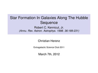
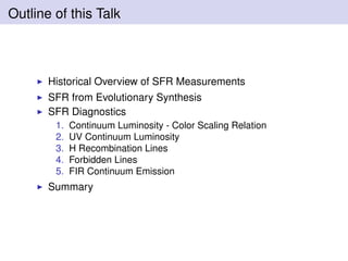
11. For Salpeter IMF 0.1 . . . 100M , continuous SFH tPop = 108 yrs:
SFR[M yr−1
] = 1.4 × 10−28
Lν[erg s−1
Hz−1
] (1)
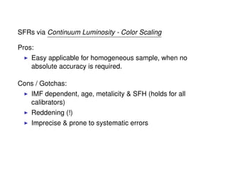
Pros:
Directly tied to photospheric emission of young-stellar
population.
Can be used for high-redshift galaxies in the optical.
Cons / Gotchas:
Not accesible from the ground for local galaxies.
Sensitive to extinction, form of IMF (large extrapolation,
since measured M > 5M )
Inappropriate e.g. for young (t ∼ 107yrs) star-burst (lower
SFR/Lν ratio, i.e. less luminos for same SFR)

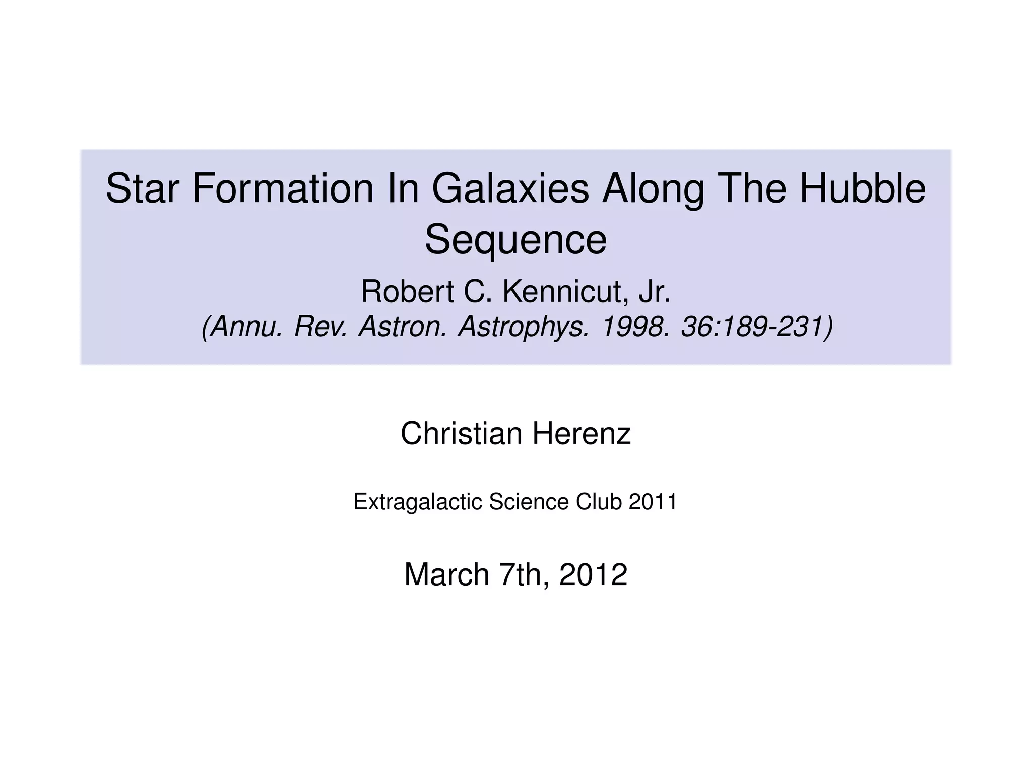
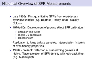
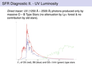
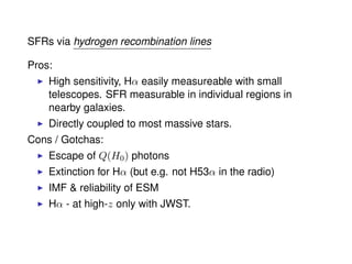
12. SFR Diagnostic III. - H Recombination Lines
Direct Tracer: Only M > 10M stars (i.e. t < 2 × 107yr)
contribute signifcantly to F(λ < 912 ˚A).
200Å 2000Å 3000Å 4000Å912Å
Λ
FΛ
For Salpeter IMF 0.1 . . . 100M , continuous SFH tPop = 108 yrs:
SFR[M yr−1
] = 1.08 × 10−53
Q(H0)[s−1
] (2)
Q(H0
)ˆ= photons with λ < 912 ˚A

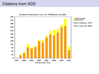
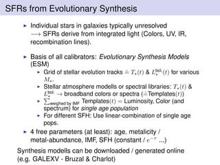
13. From Eq. (2), using your “favorite recombination scenario”,
line-strengths can be derived (e.g. using tables compiled in
Osterbrock’s monograph).
For example for Case B recombination with Te = 10, 000 K:
SFR[M yr−1
] = 7.9 × 10−42
L(Hα) [erg s−1
] (3)
= 8.2 × 10−53
L(Brγ) [erg s−1
] (4)
= . . .
⇒ Recombination Lines ˆ= “Ionizing Photon Counters” (under
certain assumptions).
Parenthesis: Case B Recombination
Gas region optically thick in Lyman-Lines (generally all gas regions
that contain enough gas to be observable - because of high Lyn
line-absorption cross section - because ∝ ψi| − er|ψf
- because of . . . )

14. SFRs via hydrogen recombination lines
Pros:
High sensitivity, Hα easily measureable with small
telescopes. SFR measurable in individual regions in
nearby galaxies.
Directly coupled to most massive stars.
Cons / Gotchas:
Escape of Q(H0) photons
Extinction for Hα (but e.g. not H53α in the radio)
IMF & reliability of ESM
Hα - at high-z only with JWST.

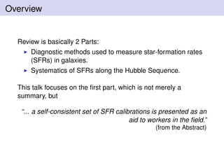
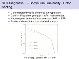
15. Forbidden Lines ([OII])
z ∼ 0.5 Hα λ6563 shifts to IR → interest in strong bluer
lines ⇒ [OII] λ3727 (doublet).
Excitation dependent on abundance and ionization state of
gas, i.e. not directly coupled to ionizing flux.
Empirical calibration to Hα Eq. 3 (using a set of ∼ 170
galaxies) yields:
SFR[M yr−1
] = (1.4 ± 0.4) × 10−41
L([OII]) [erg s−1
] (5)
Pros: bluer, stronger Cons: Less precise

16. FIR Continuum
Simplest Case: Radiation field dominated by young stars,
dust opacity high everywhere (dusty circumnuclear
starburst)
Dust: Absorbs essentially bolometric luminosity and
re-emits it as thermal emission (i.e. calorimetric SFR
measure).
Real Situation more complex - e.g. τ 1 approximation
not valid, dust needs to depleted by stars (i.e. old
generation contributes to dust heating) - etc.
Models from literature calibrated to IMF used for other
relations (±30%):
SFR[M yr−1
] = 4.5 × 10−44
LFIRo(8 − 1000µm) [erg s−1
]
(6)
10 – 100 Myr old starburst

17. Summary
Several tracers (UV, Lines, FIR) for SFR exist, but quantitative
calibration is tricky and requires a set of assumptions. Provided
that for a galaxy or sample of galaxies the assumptions given in
this review are valid, the formulas
SFR[M yr−1
] = 1.4 × 10−28
Lν[erg s−1
Hz−1
]
SFR[M yr−1
] = 7.9 × 10−42
L(Hα) [erg s−1
]
= 8.2 × 10−53
L(Brγ) [erg s−1
]
= . . .
SFR[M yr−1
] = (1.4 ± 0.4) × 10−41
L([OII]) [erg s−1
]
SFR[M yr−1
] = 4.5 × 10−44
LFIRo(8 − 1000µm) [erg s−1
]
can be used.