1. JOURNAL OF THE SOUTHEASTERN ASSOCIATION FOR RESEARCH IN ASTRONOMY, 2, 14-18, 2008 MAY 1
c 2008. Southeastern Association for Research in Astronomy. All rights reserved.
SCATTERING POLARIZATION OF ARBITRARY ENVELOPES BY ANISOTROPIC STELLAR ILLUMINATION
J. C. CARSON
1
Department of Physics and Astronomy, Western Kentucky University, KY 42101
AND
R. IGNACE
Department of Physics, Astronomy, and Geology, Johnson City, TN 37614
ABSTRACT
We model the polarization arising from electron scattering of light by a circumstellar envelope of an arbitrary
shape. This is accomplished by describing the scattering function, stellar flux, and envelope density distribu-
tion in general terms using spherical harmonics and then applying their orthogonality relationships in integral
expressions that describe the net observed polarization. We then take a specific example of a uniform stellar
light source surrounded by an ellipsoidal shell. As an example, a polarization of 25 percent is found for the
case of a disk-like star that is viewed edge-on and that is surrounded by a a disk-like envelope oriented viewed
face-on to the observer.
Subject headings: Polarization, Thomson Scattering, Rayleigh Scattering
1. INTRODUCTION
Observed linear polarizations from most stars is mainly pro-
duced by scattering on circumstellar matter. There have been
many papers written about the analytic treatment of polariza-
tion and scattered flux. In a seminal paper, Brown & Mclean
(1977) assumed an unpolarized isotropic point source and an
axisymmetric circumstellar envelope. For Thomson scatter-
ing they found that the percentage polarization was depen-
dent upon a shape factor for the envelope, the envelope optical
depth, and the inclination angle of the system in the observer;s
frame. Since then many other treatments have been consid-
ered such as the generalization by Simmons (1982, 1983) for
the case of Mie and Rayleigh Scattering . There has also
been treatment of the case of multiple isotropic point sources
(Brown, Mclean & Emslie 1978)
The past theories have one thing in common: they con-
sider only isotropic sources. However, stars in general are
anisotropic light sources. This anisotropy arises mainly
through two effects: the star being non-spherical in shape or
surface blemishes such as sunspots. In this paper we deal with
the case of an unresolved nonspherical source, surrounded by
a ellipsoidal circumstellar shell. An initial study by Al-Malki
et al. (1999) presented results for a non-isotropic source in a
spherical envelope. In Al-Malki’s et al., a maximum polar-
ization was received of about 20% for a disk-like star was
achieved. In this paper a somewhat higher maximum polar-
ization of about 25% is found for a disk-like star embedded in
a disk-like envelope.
In section 2 we present the general expression for the scat-
tered flux and polarization in intergal form and define the
three reference frames present within our system. We then de-
compose these expressions through the use of spherical har-
monics. In section 3 we apply the model discussed in sec-
tion 2 to the case of a small non-spherical blackbody star sur-
rounded by an ellipsoidal shell. An approximation is consid-
ered and a maximum polarization is found for the case of a
disk-like star viewed edge-on and a disk-like star view face-
1 Southeastern Association for Research in Astronomy (SARA) NSF-REU
Summer Intern
Electronic address: Jason.Carson@wku.edu; ignace@etsu.edu
on. In section 4 we consider a specific example of a binary
star system surrounded by an ellipsoidal shell. We conclude in
section 5 with a discussion of improvements needed to make
the model more complete.
2. GENERAL EXPRESSION FOR SCATTERED FLUX AND
POLARIZATION
We first need to consider the fact that there are three refer-
ence frames we will be dealing with in this paper: one for the
envelope, one for the star, and one for the observer. The origin
for each of these will be at the star center, hence the spherical
radius r from the star center to any point in the envelope will
have the same magnitude in all three frames. The following
describes the three separate coordinate systems.
i) For the observer reference frame we define a carte-
sian coordinate system (x,y,z) centered at the star, with
spherical coordinates (r,θ,φ), with the line-of-sight be-
ing the Oz−axis. Thus ˆz is a unit vector in the direction
of the observer from the star and x,y are observer coor-
dinates in the plane of the sky. For a scattering point in
direction ˆr, the scattering angle is given by cosθ = ˆz· ˆr,
as in Al-Malki et al. (1999). The angle φ = tan−1
y/x is
the observer’s polarization angle (orientation) relative
to Oz for any scattering point.
ii) The star’s frame (X,Y,Z) with spherical coordinates
(r,ϑ,ϕ), where OZ is a convenient stellar axis (such as
a rotation axis) that lies in the x − z plane of the ob-
server’s frame. The star system is rotated relative to
observer coordinates (x,y,z) through standard Euler an-
gles (α,β,γ).
iii) The envelope frame (X ,Y ,Z ) with spherical coordi-
nates (r,ϑ ,ϕ ),centered on the star, where OZ is an
axis of symmetry for the enevelope.
In general the density of scatterers is n(r,ϑ ,ϕ ), and the flux
of the radiation from the star that is taken to be unpolarized
is described by F(r,ϑ,ϕ). Following Al-Malki et al. (1999),
equation (1) gives the Stokes parameters of the scattered radi-
ation as:

2. Scattering Polarization of Abitrary Envelopes by Anistropic Stellar Illumination 15
Fsc
Z∗ =
1
2k2 D2
n(r,θ ,φ )F(r,ϑ,ϕ)r2
×
(i1 +i2)
(i1 −i2) exp(−2iφ)
dr sinθdθdφ, (1)
with Z∗
= Q−iU ( where Q and U are the linear stokes param-
eters), i =
√
−1, k = 2π/λ the wave number, and i1 and i2 the
scattering functions as defined by van de Hulst (1957). For
Thomson (free electrons) or Rayleigh scattering, we have
i1 ±i2 =
3k2
8π
σ(1±cos2
θ), (2)
where the value of the cross section factor σ is chosen ac-
cording to whether Thomson scattering (σ ∝ k2
) or Rayleigh
scattering (σ ∝ k4
) is being considered.
Providing that F varies smoothly, it may be conveniently
expressed in terms of spherical harmonics in the observer
frame (θ,φ),
F(r,θ,φ) =
∞
l=0
m=l
m=−l
Flm(r)
n=l
n=−l
R(l)
nm(α,β,γ)Yln(ϑ,ϕ), (3)
where R(l)
nm are rotation matrices described by Messiah (1962).
Generally, we can expand the density distribution of scatter-
ers in terms of spherical harmonics, which for the observer’s
frame becomes
n(r,θ,φ) =
∞
l =0
m =l
m =−l
nl m (r)Yl m (θ,φ). (4)
Using the properties of the product of two spherical har-
monics (Messiah 1962), we can express the multipoles of
n(r,θ,φ) and F(r,θ,φ) as:
n(r,θ,φ)F(r,θ,φ) =
lmn
Rl
nm
l m
CLM
ll nm YLM(θ,φ). (5)
In this past expression, the factors CLM
ll nm are Clebsh-Gordon
coefficients, arising from the products of two spherical har-
monics. Only terms satisfying the following two conditions
contribute to the sum in Equation 5:
n+m = M, (6)
and,
|l −l | ≤ l ≤ l +l . (7)
The coefficients are given, using Racah notation, by
CLM
ll nm =(−1)M (2l +1)(2l +1)(2L+1)
4π
×
l l L
0 0 0
l l L
nm M
(8)
(c.f., Messiah 1962, where values of the Clebsh-Gordon coef-
ficients and the rotation martices are tabulated).
In order to exploit the orthogonality properties of spherical
harmonics we must express the factors in the scattering func-
tion also in terms of spherical harmonics.
(i1 +i2) ∝ 1+cos2
θ =
4
3
√
4πY00 +
π
5
Y20(θ) , (9)
and
(i1 +i2) ∝ sin2
θ exp(−2iφ) = 4
√
2π
15
Y∗
22(θ,φ), (10)
So once substituted into the integrals contained in Equation 1,
together with the other expressions above, and using the prop-
erties of spherical harmonics, Fsc and Z∗
can be rewritten as:
Fsc =
σ
4πD2
lmn
Rl
nm(α,β,γ)
×
√
4πC00
ll nm +
π
5
C20
ll nm Sll mm , (11)
and
Rl
nm(α,β,γ)
l m
C22
ll nm Sll mm , (12)
where
Sll mm =
∞
0
Flm(r)nl m (r)r2
dr, (13)
with
Flm(r) =
1
−1
2π
0
F(r,θ,φ)Y∗
lm(θ,φ)d(cosθ)dφ, (14)
and
nl m (r) =
1
−1
2π
0
n(r,θ ,φ )Y∗
l m (θ ,φ )d(cosθ )dφ . (15)
Equations 14 and 15 describe the effects of each function (F
and n) in the appropriate stellar or envelope frame (c.f., Sim-
mons 1982).
If the functions are smooth, the summations will converge
rapidly, so the first few terms with l and l ≤ 2 will give rea-
sonable approximations. Due to the conditions of Equations
6 and 7, the summation over l,l , m, and m’ in Equations
11 and 12 will be limited. For functions describing the stel-
lar flux and the circumstellar density distribution of scattering
particles symmetrically about stellar and envelope polar axes,
respectively, the values of Sll mm will be zero for odd values
of l and l .
For a spherical envelope with n(r,θ,φ) = n(r) and an
anisotropic light source, Equations 11 and 12 reduce to the
forms discussed in Al-Malki et al. (1999). On the other hand,
for an isotropic light source within an axisymmetric enevlope,
the expressions of Brown & McLean (1977) and Simmons
(1982) are recovered.
3. ELLIPSOIDAL LIGHT SOURCE AND ELLIPSOIDAL
CIRCUMSTELLAR ENVELOPE
As an illustration of the preceding general formulation, we
will take the case of a small blackbody star of uniform surface
temperature embedded within an ellipsoidally shaped circum-
stellar envelope. For such a star of isotropic surface intensity
I∗, the flux F(r,ϑ,ϕ) can be expressed in terms of the pro-
jected area Ap(ϑ,ϕ) of the star as seen from direction (ϑ,ϕ).
The flux is given by
F∗(r,ϑ,ϕ) ≈ I∗ ∆Ω = I∗
Ap(ϑ,ϕ)
r2
, (16)

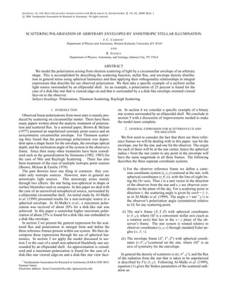
3. 16 J.Carson et al.
Z
X
Y
z
To Earth
c
a
b
φ
s
i
Axis
Rotation
FIG. 1.— The ellipsoidal star coordinate system, where the c-axis is along
the Z-axis (i.e., the rotation axis.)
where I∗ is the isotropic intensity of the stellar surface and ∆Ω
is the solid angle subtended by the scattering element located
a distance r from the star. For this star we define axes (a,b,c)
to be along (X,Y,Z) (see Figure 1). The Ap function is defined
by the following:
Ap = π (bcλ)2 +(acµ)2 +(abν)2 , (17)
where (λ,µ,ν) = (cosϕsinϑ,sinϕsinϑ,cosϑ) are the (X,Y,Z)
direction cosines. So we obtain finally,
Flm(r) =
I∗
r2
π
0
2π
0
Ap(ϑ,ϕ)Y∗
lm(ϑ,ϕ) sinϑdϑdϕ. (18)
We take the circumstellar envelope to be the same as that
of Simmons (1982), an ellipsoidal shell of arbitrary thickness
and uniform density. The density distribution, which has an
axis of rotational symmetry OZ , has an inclination angle ie
with the line of sight. We shall consider only the case of rota-
tion of OZ about the line of sight, but not any other direction,
with an azimuthal angle φe in the observer frame (see Figure
2). We then have (Simmons 1982):
nl m (r) = 2π(R1 −R2)n0 Kl Yl m (ie,φe). (19)
RR
R /A
ie
2 1
1 r
2R /Ar
Toward Observer
X’
Y’
Z’
z
FIG. 2.— Definitions of R1, and R2 . This figure further defines the coordi-
nate system and geometry of the ellipsoidal shell.
The outer and inner radii of the shell are, respectively,
r1,2(µ) =
R1,2
1+(A2
r −1)µ2
, (20)
where
µ = cosζ. (21)
The lengths R1 and R2 are the outer and inner equatorial axis
length, and Ar is the ratio of the length of the equatorial axis
to the polar axis (see Figure 2). The angle ζ is the angle be-
tween the radius vector and the axis of symmetry, OZ , which
is related to our frames by the addition theorem of spherical
harmonics. (This explains the appearance of Yl m (ie,φe) in
Equation 19 – see Simmons 1982 and Jackson 1975.) Finally,
Kl values represent moments of the envelope. They can be
related to the shape factor found in Brown & Mclean (1977)
and are given by :
Kl =
1
−1
Pl (µ)
1+(A2
r −1)µ2
dµ. (22)
Inserting equations (18) to (22) in Eq. (13), we obtain
Sll mm = I∗ N flm Kl Yll m (ie,φe), (23)
where we have defined a column density
N = 2π(R1 −R2)n0, (24)
and
flm =
π
0
2π
0
Ap(ϑ,ϕ)Y∗
lm(ϑ,ϕ) sinϑdϑdϕ. (25)
Note that the spherical harmonic decomposition coefficients
of the flux flm are now functions of the star’s shape and size
only (i.e., of a,b, and c). Moreover, the spherical harmonic
decomposition coefficients of the envelope Kl are also func-
tions of the envelope’s shape and size only (i.e., of Ar). This
combination of Kl and flm determines the polarization and
the scattered flux, depending on whether the two functions
enhance or offset one another.
If we describe the orientation of the star relative to the ob-
server frame in terms of the Euler angles, then we can choose
α as zero, β = is is the viewing inclination of the OZ−axis
(i.e., the rotation axis of the star) to the line of sight Oz−axis,
and γ = φs as the azimuth of the OZ−axis from the Ox−axis
as measured about the Oz−axis. Thus φs measures the rota-
tional position or phase of the star relative to the observer (see
Figure 3).
For the observational situation, the normalized scattered
flux and Stokes parameters are usually used. They are given
by (fsc,q,u) = (Fsc,Q,U)/Ftot, where the total flux received
Ftot comprises the combination of the scattered flux Fsc plus
direct flux from the star. This contribution by direct stellar
light we denote as F∗ = I∗ Ap(is,φs)/D2
. So the total observed
flux becomes
Ftot =
I∗
D2
Ap(is,φs)+(D2
/I∗)Fsc . (26)
The general expressions for the normalized scattered flux and
stokes parameters become

4. Scattering Polarization of Abitrary Envelopes by Anistropic Stellar Illumination 17
P
P’
φAxis of
Star
Axis of
Observation
Y
y
x
Z
z
O
defined by z and Z
Lies in plane
X
FIG. 3.— Definitions of the star’s and observers coordinate systems. The
point O marks the emitting anisotropic star (point source), and P a general
scattering particle in the envelope. OZ is the rotation axis, where θ is the
scattering angle, and φ is the polarization direction. The Euler angles are
α = 0, β = is the inclination angle between Oz and OZ, and γ = φs the angle
from the X-axis in the xy-plane. The scattering plane is P OP.
fsc =
τ
4πFtot
lmn
Rl
nm(0,is,φs) flm
×
√
4πC00
ll nm +
π
5
C20
ll nm (27)
and with z∗
= q−iu,
z∗
=
3τ
4πFtot
2π
15
lmn
Rl
nm(0,is,φs) flm
l m
Kl Yl m(ie,φe)C22
ll nm Sll mm , (28)
where τ is the average envelope optical depth, equal to
σ(R1 − R2)n0 (see Simmons 1982). The degree of polariza-
tion is given by p = |z∗
| = |z| = q2 +u2, and the polarization
direction is given by φp = 1
2 tan−1
(u/q).
From Equations 27 and 28, we can calculate the polariza-
tion and the scattered flux, using the properties of the two
factors Kl and flm, that describe the envelope and stellar
anisotropy. The stellar flux and the scatterer density func-
tions, Kl and flm are non-zero only for even values of l and
l.
4. APPLICATIONS
We now examine the theory in more detail and create an
approximation that can be applied to many cases. As previ-
ously noted, the multipoles of the flux flm are non-zero only
for even l, and the spherical harmonics for l ≥ 4 are important
only for fairly large stellar distortions from sphericity. For
most values of c, f20 domintes fl0 for l ≥ 2 . We therefore
neglect the effects of flm for l > 2.
For l = l = 2, we can write the scattered flux as
Fsc =
σ
4πD2
√
4π
m=2
m=−2
S222−2
m C00
222−2
+
m=2
m=−2
S221−1
m C00
221−1 +
m=2
m=−2
S2200
m C00
2200
+
m=2
m=−2
S22−11
m C00
22−11 +
m=2
m=−2
S22−22
m C00
22−22
+S0000
m C00
0000 +
π
5
S0200
0 C20
0200
+
m=2
m=−2
S222−2
m C20
222−2 +
m=2
m=−2
S221−1
m C20
221−1
+
m=2
m=−2
S2200
m C20
2200 +
m=2
m=−2
S22−11
m C20
22−11
+
m=2
m=−2
S22−22
m C20
22−22 +
m=2
m=−2
S2000
m C20
2000 , (29)
and the Stokes parameters as
z∗
=
3σ
4πD2
2π
15
S0202
0 C22
0202
+
m=2
m=−2
S2220
m C22
2220 +
m=2
m=−2
S2211
m C22
2211
+
m=2
m=−2
S2202
m C22
2202 +
m=2
m=−2
S2020
m C22
2020 , (30)
where
Sll nm
m = Rl
nm(α,β,γ)Sll mm . (31)
In the case of a spherical envelope and a disk-like star (a = b =
1,c = 0) , a polarization of p20% is theoretically achievable
(Al-Malki et al. 1999). Our more general model does repro-
duce this value for a spherical envelope. As an extreme case
to investigate large polarization values, we use the disk star
example of Al-Malki et al. but now with a disk-shaped enve-
lope. A maximu polarization of about 25 % is produced for
the disk-shaped star (a = b = 1 and c = 0) viewed edge-on at
is = 90◦
with disk-shaped envelope that is oriented face-on to
the observer (ie = 0◦
) and orthogonal to the star. Note that as
long as the envelope is optically thin, the quoted polarization
values for these extreme cases are independent of the envelope
optical depth τ.
We have considered applications of equations (29) and
(30) to a single fast rotating oblate star, a Roche lobe fill-
ing star, and a non-radially oscillating star. The results yield
qu−diagrams of similar shape as in the spherical envelope
case of Al-Malki et al. (1999), but with smaller or larger val-
ues of q and u. The main difference is that the two functions of
F and n for the star flux and envelope density distribution can
enhance or offset each other. These models will be discussed
in a separate paper.
5. CONCLUSION
In this work a model for the polarization arising from an
anisotropic point light source within an arbitraryily shaped en-
velope has been presented. We specifically considered Thom-
son and Rayleigh scattering mechanisms. The mathematical
analysis made full use of spherical harmonics decomposition

5. 18 J.Carson et al.
and their properties. By using the first few spherical harmon-
ics, an acceptable approximation was derived to represent star
and envelope distortions by substantial amounts. The applica-
tion of the general model to a disk-like star with zero thickness
viewed edge-on surrounded by a disk-like envelope oriented
pole-on to the observer gave a polarization of 25%.
In the future we would like the effects of the finite star
size, effects that tend to lower the net polarization (Cassinelli,
Nordsieck, & Murison 1987). We have started to include
these effects in the specific case of a cool, evolved star to
model a laterally structured chromosopheric envelope (Ig-
nace, Henson, & Carson 2007), but the approach has not yet
been generalized.
This project was funded by a partnership between the Na-
tional Science Foundation (NSF AST-0552798), Research
Experiences for Undergraduates (REU), and the Department
of Defense (DoD) ASSURE (Awards to Stimulate and Sup-
port Undergraduate Research Experiences) programs. We
would also like to thank Dr. Gary Henson for his many helpful
discussions.
REFERENCES
Al-Malki, M. B., Simmons, J. F. L., Ignace, R., Brown, J. C., Clarke, D.,
1999, A&A 347, 919
Brown, J. C., McLean, I. S., 1977, A&A 57, 141
Brown, J. C., McLean, I. S., Emslie, A. G., 1978 A&A 68, 415
Cassinelli, J.P., Nordsieck, K.H., Murison, M.A., 1987, ApJ, 317, 293
Ignace, R., Henson, G. D., Carson, J. C., 2007 to appear in Biggest, Baddest,
Coolest Stars, (eds) Luttermoser, Smith, Steneil
Jackson, J. D., 1975, Classical Electrodynamics, 2nd ed., J. Wiley & Son,
New York
Karovska, M., Nisenson, P., Papaliolios, C., 1992, Sky & Telescope 83, 130
Messiah, A., 1962, Quantum Mechanics VII, North-Holland Publishing
Company, Amsterdam
Simmons, J. F. L., 1982, MNRAS 200, 91
Simmons, J. F. L., 1983, MNRAS 205, 153
van de Hulst, H. C., 1957, Light Scattering by Small Particles, (New York:
John Wiley & Sons)