Download as PDF, PPTX
![O(3) Sigma Model on the Euclidean Plane
We consider space-time R1,2
with signature (+, −, −). Let
ϕ : R1,2
→ S2
, a ∈ Ω1
(
R1,2
)
and let us fix n ∈ S2
such that we can
define the height ϕ3 = ϕ · n. The abelian O(3) sigma model is given by
the functional
∫
R2
1
2
Dµϕ · Dµ
ϕ −
1
4
fµνfµν
−
1
2
(τ − ϕ3)
2
d2
x, (1)
where,
Dµϕ = ∂µϕ − aµn × ϕ, (2)
is the covariant derivative on the trivial fibered bundle R1,2
× S2
associated with the connection form and the real constant τ is chosen in
the interval [−1, 1].
EIG-GR 2019 June 10th - 12th, Granada, Spain. 3 / 38](https://image.slidesharecdn.com/presentacion-granada-190608183611/85/Presentacion-granada-3-320.jpg)
![Approximated dynamics on moduli space
1. If a system of vortices and antivortices is moving slowly, it can be
approximated to some degree by parametric motion on moduli space.
2. We make the assumption that stationary solutions dependent on a
real parameter are approximations to truly dynamical solutions to
the field equations.
3. This assumption has been thoroughly tested for Ginzburg-Landau
vortices [2].
EIG-GR 2019 June 10th - 12th, Granada, Spain. 16 / 38](https://image.slidesharecdn.com/presentacion-granada-190608183611/85/Presentacion-granada-16-320.jpg)
![Geometry on compact domains
Let Σ be a closed surface with a Riemannian metric g and compatible
pseudocomplex structure. A construction by Sibner et al. [3] extends the
fields to take values on a fiber bundle with base Σ and fibers S2
. This
construction is further generalized in the work of Romao and Speight [1].
We can extend the previous discussion about the O(3) Sigma model to
R × Σ with the metric dt2
− g.
EIG-GR 2019 June 10th - 12th, Granada, Spain. 23 / 38](https://image.slidesharecdn.com/presentacion-granada-190608183611/85/Presentacion-granada-23-320.jpg)
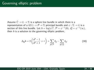
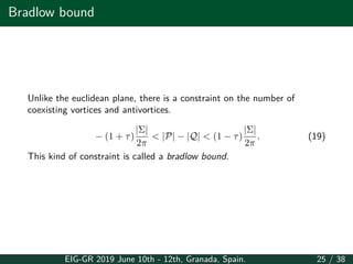
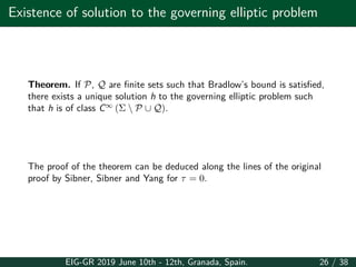
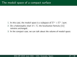
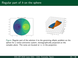
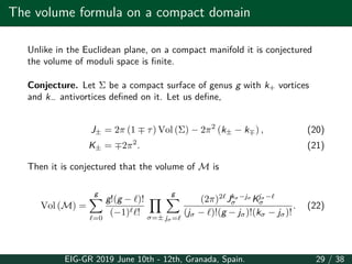
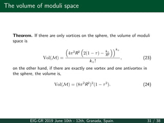


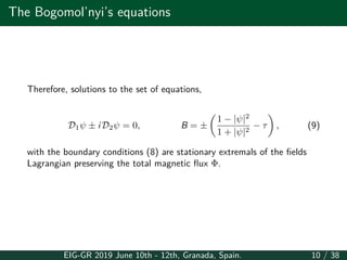
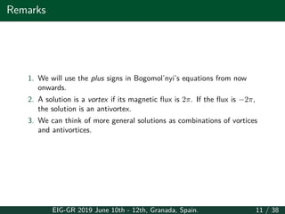
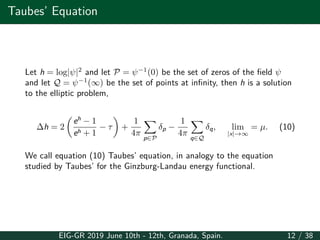
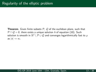
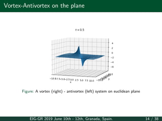
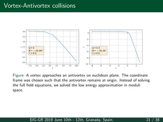
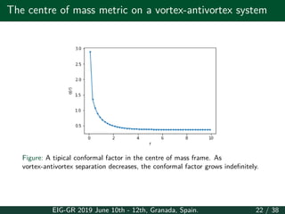
This document summarizes a presentation about the moduli space of BPS vortex-antivortex pairs. It discusses the O(3) sigma model on Euclidean space and compact domains. On Euclidean space, it derives Bogomol'nyi's equations and Taubes' equation to describe stationary solutions. It discusses the moduli space and derives a localization formula for the metric on moduli space. It also discusses vortex-antivortex collisions and the behavior of the conformal factor. On compact domains, it discusses an elliptic problem to describe solutions and derives a Bradlow bound on the number of vortices and antivortices.


