Download free for 30 days
Sign in
Upload
Language (EN)
Support
Business
Mobile
Social Media
Marketing
Technology
Art & Photos
Career
Design
Education
Presentations & Public Speaking
Government & Nonprofit
Healthcare
Internet
Law
Leadership & Management
Automotive
Engineering
Software
Recruiting & HR
Retail
Sales
Services
Science
Small Business & Entrepreneurship
Food
Environment
Economy & Finance
Data & Analytics
Investor Relations
Sports
Spiritual
News & Politics
Travel
Self Improvement
Real Estate
Entertainment & Humor
Health & Medicine
Devices & Hardware
Lifestyle
Change Language
Language
English
Español
Português
Français
Deutsche
Cancel
Save
EN
AM
Uploaded by
Akira Maruoka
PPTX, PDF
372 views
Prelude to Halide
Halide勉強会(2018/07/28) @Fixstars の発表資料です。 https://halide-ug.connpass.com/event/91556/
Engineering
◦
Read more
4
Save
Share
Embed
Embed presentation
Download
Download to read offline
1
/ 56
2
/ 56
3
/ 56
4
/ 56
5
/ 56
6
/ 56
7
/ 56
8
/ 56
9
/ 56
10
/ 56
11
/ 56
12
/ 56
13
/ 56
14
/ 56
15
/ 56
16
/ 56
17
/ 56
18
/ 56
19
/ 56
20
/ 56
21
/ 56
22
/ 56
23
/ 56
24
/ 56
25
/ 56
26
/ 56
27
/ 56
28
/ 56
29
/ 56
30
/ 56
31
/ 56
32
/ 56
33
/ 56
34
/ 56
35
/ 56
36
/ 56
37
/ 56
38
/ 56
39
/ 56
40
/ 56
41
/ 56
42
/ 56
43
/ 56
44
/ 56
45
/ 56
46
/ 56
47
/ 56
48
/ 56
49
/ 56
50
/ 56
51
/ 56
52
/ 56
53
/ 56
54
/ 56
55
/ 56
56
/ 56
More Related Content
PPTX
DIC-PCGソルバーのpimpleFoamに対する時間計測と高速化
by
Fixstars Corporation
PDF
Halide による画像処理プログラミング入門
by
Fixstars Corporation
PDF
OpenFOAMスレッド並列化のための基礎検討
by
Fixstars Corporation
PDF
Halide for Memory
by
Koumei Tomida
PDF
TVM の紹介
by
Masahiro Masuda
PPTX
XLWrapについてのご紹介
by
Ohsawa Goodfellow
PDF
CMSI計算科学技術特論B(11) 大規模MD並列化の技術2
by
Computational Materials Science Initiative
PPT
A Multiple Pairs Shortest Path Algorithm 解説
by
Osamu Masutani
DIC-PCGソルバーのpimpleFoamに対する時間計測と高速化
by
Fixstars Corporation
Halide による画像処理プログラミング入門
by
Fixstars Corporation
OpenFOAMスレッド並列化のための基礎検討
by
Fixstars Corporation
Halide for Memory
by
Koumei Tomida
TVM の紹介
by
Masahiro Masuda
XLWrapについてのご紹介
by
Ohsawa Goodfellow
CMSI計算科学技術特論B(11) 大規模MD並列化の技術2
by
Computational Materials Science Initiative
A Multiple Pairs Shortest Path Algorithm 解説
by
Osamu Masutani
What's hot
PPTX
強化学習アルゴリズムPPOの解説と実験
by
克海 納谷
PDF
研究動向から考えるx86/x64最適化手法
by
Takeshi Yamamuro
PDF
XLWrapについてのご紹介
by
Ohsawa Goodfellow
PDF
CMSI計算科学技術特論B(4) アプリケーションの性能最適化の実例1
by
Computational Materials Science Initiative
PDF
CMSI計算科学技術特論B(5) アプリケーションの性能最適化の実例2
by
Computational Materials Science Initiative
PDF
CMSI計算科学技術特論B(10) 大規模MD並列化の技術1
by
Computational Materials Science Initiative
PDF
LLVMで遊ぶ(整数圧縮とか、x86向けの自動ベクトル化とか)
by
Takeshi Yamamuro
PPTX
20180728 halide-study
by
Fixstars Corporation
PDF
浮動小数点(IEEE754)を圧縮したい@dsirnlp#4
by
Takeshi Yamamuro
PDF
C base design methodology with s dx and xilinx ml
by
ssuser3a4b8c
PDF
20180109 titech lecture_ishizaki_public
by
Kazuaki Ishizaki
強化学習アルゴリズムPPOの解説と実験
by
克海 納谷
研究動向から考えるx86/x64最適化手法
by
Takeshi Yamamuro
XLWrapについてのご紹介
by
Ohsawa Goodfellow
CMSI計算科学技術特論B(4) アプリケーションの性能最適化の実例1
by
Computational Materials Science Initiative
CMSI計算科学技術特論B(5) アプリケーションの性能最適化の実例2
by
Computational Materials Science Initiative
CMSI計算科学技術特論B(10) 大規模MD並列化の技術1
by
Computational Materials Science Initiative
LLVMで遊ぶ(整数圧縮とか、x86向けの自動ベクトル化とか)
by
Takeshi Yamamuro
20180728 halide-study
by
Fixstars Corporation
浮動小数点(IEEE754)を圧縮したい@dsirnlp#4
by
Takeshi Yamamuro
C base design methodology with s dx and xilinx ml
by
ssuser3a4b8c
20180109 titech lecture_ishizaki_public
by
Kazuaki Ishizaki
Similar to Prelude to Halide
PDF
HalideでつくるDomain Specific Architectureの世界
by
Fixstars Corporation
PPTX
計算スケジューリングの効果~もし,Halideがなかったら?~
by
Norishige Fukushima
PPTX
画像処理の高性能計算
by
Norishige Fukushima
PPT
Or seminar2011final
by
Mikio Kubo
PDF
Fpga online seminar by fixstars (1st)
by
Fixstars Corporation
PDF
実務者のためのかんたんScalaz
by
Tomoharu ASAMI
PDF
携帯SoCでの画像処理とHalide
by
Morpho, Inc.
PDF
Object-Functional Analysis and Design : 次世代モデリングパラダイムへの道標
by
Tomoharu ASAMI
PPT
Rpscala2011 0601
by
Hajime Yanagawa
PDF
Halide, Darkroom - 並列化のためのソフトウェア・研究
by
Yuichi Yoshida
PDF
optimal Ate pairing
by
MITSUNARI Shigeo
PDF
PCD2019 TOKYO ワークショップ「2時間で!Processingでプログラミング入門」
by
reona396
PDF
R-hpc-1 TokyoR#11
by
Shintaro Fukushima
PDF
Scalaプログラミング・マニアックス
by
Tomoharu ASAMI
PDF
Object-Funcational Analysis and design
by
Tomoharu ASAMI
PDF
マルチレイヤコンパイラ基盤による、エッジ向けディープラーニングの実装と最適化について
by
Fixstars Corporation
PDF
Processing
by
Akifumi Nambu
PDF
[Basic 13] 型推論 / 最適化とコード出力
by
Yuto Takei
PDF
Rの高速化
by
弘毅 露崎
PPTX
20160723 オープンキャンパス資料
by
Takeo Kunishima
HalideでつくるDomain Specific Architectureの世界
by
Fixstars Corporation
計算スケジューリングの効果~もし,Halideがなかったら?~
by
Norishige Fukushima
画像処理の高性能計算
by
Norishige Fukushima
Or seminar2011final
by
Mikio Kubo
Fpga online seminar by fixstars (1st)
by
Fixstars Corporation
実務者のためのかんたんScalaz
by
Tomoharu ASAMI
携帯SoCでの画像処理とHalide
by
Morpho, Inc.
Object-Functional Analysis and Design : 次世代モデリングパラダイムへの道標
by
Tomoharu ASAMI
Rpscala2011 0601
by
Hajime Yanagawa
Halide, Darkroom - 並列化のためのソフトウェア・研究
by
Yuichi Yoshida
optimal Ate pairing
by
MITSUNARI Shigeo
PCD2019 TOKYO ワークショップ「2時間で!Processingでプログラミング入門」
by
reona396
R-hpc-1 TokyoR#11
by
Shintaro Fukushima
Scalaプログラミング・マニアックス
by
Tomoharu ASAMI
Object-Funcational Analysis and design
by
Tomoharu ASAMI
マルチレイヤコンパイラ基盤による、エッジ向けディープラーニングの実装と最適化について
by
Fixstars Corporation
Processing
by
Akifumi Nambu
[Basic 13] 型推論 / 最適化とコード出力
by
Yuto Takei
Rの高速化
by
弘毅 露崎
20160723 オープンキャンパス資料
by
Takeo Kunishima
Prelude to Halide
1.
Prelude to Halide Akira
Maruoka Fixstars Corporation © 2018 Fixstars Corporation. All rights reserved.
2.
自己紹介 名前: 丸岡 晃
(Akira Maruoka) 所属: 株式会社フィックスターズ 専門分野: 最適化コンパイラ – 学生時代: • ループ最適化とか自動ベクトル化とかやってました • LLVMでバックエンド作ったりもしてました – お仕事: • FPGA向けのHalideコンパイラ「GENESIS」を開発してます 1 © 2018 Fixstars Corporation. All rights reserved.
3.
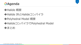
Agenda Halide 概要 Halide IRとHalideコンパイラ Polyhedral
Model 概要 HalideコンパイラでPolyhedral Model まとめ 2 © 2018 Fixstars Corporation. All rights reserved.
4.
Halide 概要 3 © 2018
Fixstars Corporation. All rights reserved.
5.
Halide[1] 画像処理の高性能計算に特化したドメイン固有言語(DSL) – http://halide-lang.org/ 特徴 – C++の内部DSLとして実装 –
アルゴリズムとスケジューリングを分離して記述 • 純粋関数型言語による簡素なアルゴリズム記述 • 計算タイミングと最適化を指定するスケジューリング記述 – 様々なHWターゲットに対する最適化・コード生成が可能 • ターゲット: x86, ARM, POWER, MIPS, NVIDIA GPGPU, Hexagon • 出力形式: LLVM-IR, C/C++, OpenCL, OpenGL, Matlab, Metal, 4 © 2018 Fixstars Corporation. All rights reserved. [1] J.Ragan-Kelley, et al, Halide: A Language and Compiler for Optimizing Parallelism, Locality, and Recomputation in Image Processing Pipelines, PLDI 2013
6.
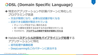
DSL (Domain Specific
Language) 特定のアプリケーションや計算パターンに特化した プログラミング言語 – 文法が簡潔になり、必要な記述量が短くなる – 記述できる範囲が限定されている • チューリング完全でない場合もある • 同一の意味を実現する記述する方法が限定されている • その代わり、プログラムの解析や変形が簡単に行える Halideはステンシル計算をパイプライニング処理する アプリケーションに特化 – 信号処理や画像処理 – DeepLearningもこのパターンに該当する 5 © 2018 Fixstars Corporation. All rights reserved.
7.
アルゴリズム記述 純粋関数型言語によって記述を行う 記述可能な表現 – 算術論理演算 – Select文による分岐式 –
リダクション計算 – 外部Cの関数呼び出し 6 © 2018 Fixstars Corporation. All rights reserved.
8.
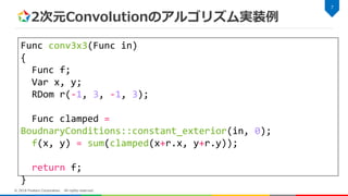
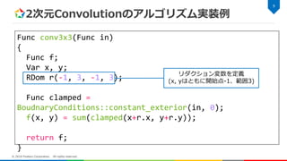
2次元Convolutionのアルゴリズム実装例 7 © 2018 Fixstars
Corporation. All rights reserved. Func conv3x3(Func in) { Func f; Var x, y; RDom r(-1, 3, -1, 3); Func clamped = BoudnaryConditions::constant_exterior(in, 0); f(x, y) = sum(clamped(x+r.x, y+r.y)); return f; }
9.
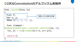
2次元Convolutionのアルゴリズム実装例 8 © 2018 Fixstars
Corporation. All rights reserved. Func conv3x3(Func in) { Func f; Var x, y; RDom r(-1, 3, -1, 3); Func clamped = BoudnaryConditions::constant_exterior(in, 0); f(x, y) = sum(clamped(x+r.x, y+r.y)); return f; } 関数と次元変数を定義
10.
2次元Convolutionのアルゴリズム実装例 9 © 2018 Fixstars
Corporation. All rights reserved. Func conv3x3(Func in) { Func f; Var x, y; RDom r(-1, 3, -1, 3); Func clamped = BoudnaryConditions::constant_exterior(in, 0); f(x, y) = sum(clamped(x+r.x, y+r.y)); return f; } リダクション変数を定義 (x, yはともに開始点-1、範囲3)
11.
2次元Convolutionのアルゴリズム実装例 10 © 2018 Fixstars
Corporation. All rights reserved. Func conv3x3(Func in) { Func f; Var x, y; RDom r(-1, 3, -1, 3); Func clamped = BoudnaryConditions::constant_exterior(in, 0); f(x, y) = sum(clamped(x+r.x, y+r.y)); return f; } 範囲外参照時の値を指定 (今回は 0 padding)
12.
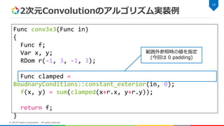
2次元Convolutionのアルゴリズム実装例 11 © 2018 Fixstars
Corporation. All rights reserved. Func conv3x3(Func in) { Func f; Var x, y; RDom r(-1, 3, -1, 3); Func clamped = BoudnaryConditions::constant_exterior(in, 0); f(x, y) = sum(clamped(x+r.x, y+r.y)); return f; } 関数fのアルゴリズムを定義
13.
スケジューリング記述 計算の意味を変えずにコードを変形出来る – 計算レベルやデータの保持の仕方を指定 •
計算量とメモリアクセスのトレードオフが決定される – ループ変形 • 並列化、ベクトル化 • アンロール、インターチェンジ、タイリング、 どのようなスケジューリングを適用するかはユーザーが指定する – 自動で最適化をしてくれるわけではない – 自動でスケジューリングを適用してくれる機能(Auto Scheduler[1])も 存在する 12 © 2018 Fixstars Corporation. All rights reserved. [1] R.T.Mullapudi, et al, Automatically Scheduling Halide Image Processing Pipelines, ACM SIGGRAPH 2016
14.
計算量と使用メモリ量のトレードオフ 13 © 2018 Fixstars
Corporation. All rights reserved. Func blur_x, blur_y; Var x, y; blur_x(x, y) = in(x, y) + in(x+1, y); blur_y(x, y) = (blur_x(x, y) + blur_x(x, y+1)) / 4; for (int y=0; y<height; y++) { for (int x=0; x<width; x++) { blur_x[y][x] = in[y][x] + in[y][x+1]; } } for (int y=0; y<height; y++) { for (int x=0; x<width; x++) { blur_y[y][x] = (blur_x[y][x] + blur_x[y+1][x]) / 4; } } for (int y=0; y<height; y++) { for (int x=0; x<width; x++) { blur_x[0][x] = in[y][x] + in[y][x+1]; blur_x[1][x] = in[y+1][x] + in[y+1][x+1]; } for (int x=0; x<width; x++) { blur_y[y][x] = (blur_x[0][x] + blur_x[1][x]) / 4; } } for (int y=0; y<height; y++) { for (int x=0; x<width; x++) { blur_y[y][x] = (in[x][y] + in[x+1][y] + in[x][y+1] + in[x+1][y+1]) / 4; } } compute_root compute_at compute_inline 計算量小 使用メモリ量小 アルゴリズム記述
15.
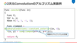
マルチターゲット向けの記述例 14 © 2018 Fixstars
Corporation. All rights reserved. Func box_filter_3x3(Func in) { Func blurx, blury; Var x, y; blurx(x, y) = (in(x-1, y) + in(x, y) + in(x+1, y))/3; blury(x, y) = (blurx(x, y-1) + blurx(x, y) + blurx(x, y+1))/3; if (get_target().has_gpu_feature()) { blury.gpu_tile(x, y, xi, yi, 32, 8); blurx.compute_at(blury, x); } else { blury.tile(x, y, xi, yi, 256, 32).vectorize(xi, 8).parallel(y); blurx.compute_at(blury, x).store_at(blury, x).vectorize(x, 8); } return blury; } アルゴリズム記述部 GPU用スケジューリング記述部 計算の本質記述と最適化のロジックが分離されている – プログラムの可読性とポータビリティが高い ターゲット毎に個別に最適化が記述出来る – マルチターゲット向けの最適化が容易に可能 CPU用スケジューリング記述部
16.
Halideの応用例 OpenCV – DNNモジュールのバックエンドに Halideが使用可能 TVM /
Tensor Comprehensions – 内部における中間表現及び コード生成に使用 Google Pixel2 – IPU(Image Processing Unit)は TensorFlowとHalideによる開発をサポート 15 © 2018 Fixstars Corporation. All rights reserved.
17.
詳しくは… Halideによる画像処理プログラミング入門 を参照 – https://www.slideshare.net/fixstars/halide-82788728 16 ©
2018 Fixstars Corporation. All rights reserved.
18.
Halide IRとHalideコンパイラ 17 © 2018
Fixstars Corporation. All rights reserved.
19.
Halide IR Halideの内部で使用されている中間表現 特徴 – 構造化プログラミング言語に近い高レベルな中間表現 –
(基本的には)データフローで完結 • ただし内部的にはコントロールフローが生成可能だったりする – 標準化されたループを生成 18 © 2018 Fixstars Corporation. All rights reserved.
20.
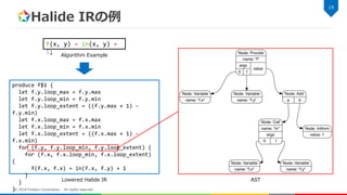
Halide IRの例 19 © 2018
Fixstars Corporation. All rights reserved. f(x, y) = in(x, y) + 1; produce f$1 { let f.y.loop_max = f.y.max let f.y.loop_min = f.y.min let f.y.loop_extent = ((f.y.max + 1) - f.y.min) let f.x.loop_max = f.x.max let f.x.loop_min = f.x.min let f.x.loop_extent = ((f.x.max + 1) - f.x.min) for (f.y, f.y.loop_min, f.y.loop_extent) { for (f.x, f.x.loop_min, f.x.loop_extent) { f(f.x, f.x) = in(f.x, f.y) + 1 } } } Algorithm Example Lowered Halide IR AST
21.
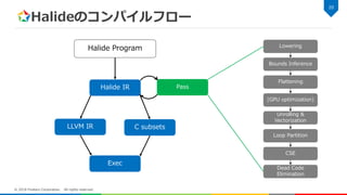
Halideのコンパイルフロー 20 © 2018 Fixstars
Corporation. All rights reserved. Halide IR LLVM IR C subsets Lowering Bounds Inference Flattening (GPU optimization) Loop Partition CSE Dead Code Elimination Halide Program Pass Exec Unrolling & Vectorization
22.
コンパイルパスに使われるクラス IRVisitor/IRGraphVisitor – IRの走査のみを行うVisitorクラス • IRの変形は行わない •
IRGraphVisitorは同じノードに対する走査は一度きりしか行わない – IRから解析情報等を構築したい場合などに使用する IRMutator – IRを走査しながら変形させるVisitorクラス – 最適化する際にはこちらを使用する 上記クラスを継承することによってパスが実装できる 21 © 2018 Fixstars Corporation. All rights reserved.
23.
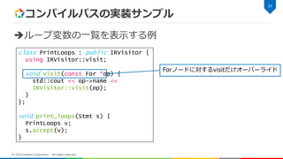
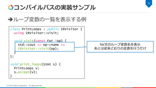
コンパイルパスの実装サンプル ループ変数の一覧を表示する例 22 © 2018 Fixstars
Corporation. All rights reserved. class PrintLoops : public IRVisitor { using IRVisitor::visit; void visit(const For *op) { std::cout << op->name << IRVisitor::visit(op); } }; void print_loops(Stmt s) { PrintLoops v; s.accept(v); }
24.
コンパイルパスの実装サンプル ループ変数の一覧を表示する例 23 © 2018 Fixstars
Corporation. All rights reserved. class PrintLoops : public IRVisitor { using IRVisitor::visit; void visit(const For *op) { std::cout << op->name << IRVisitor::visit(op); } }; void print_loops(Stmt s) { PrintLoops v; s.accept(v); } IRVisitorクラスを継承してクラスを定義
25.
コンパイルパスの実装サンプル ループ変数の一覧を表示する例 24 © 2018 Fixstars
Corporation. All rights reserved. class PrintLoops : public IRVisitor { using IRVisitor::visit; void visit(const For *op) { std::cout << op->name << IRVisitor::visit(op); } }; void print_loops(Stmt s) { PrintLoops v; s.accept(v); } Forノードに対するvisitだけオーバーライド
26.
コンパイルパスの実装サンプル ループ変数の一覧を表示する例 25 © 2018 Fixstars
Corporation. All rights reserved. class PrintLoops : public IRVisitor { using IRVisitor::visit; void visit(const For *op) { std::cout << op->name << IRVisitor::visit(op); } }; void print_loops(Stmt s) { PrintLoops v; s.accept(v); } for文のループ変数名を表示 あとは従来どおりの走査を行うだけ
27.
コンパイルパスの実装サンプル ループ変数の一覧を表示する例 26 © 2018 Fixstars
Corporation. All rights reserved. class PrintLoops : public IRVisitor { using IRVisitor::visit; void visit(const For *op) { std::cout << op->name << IRVisitor::visit(op); } }; void print_loops(Stmt s) { PrintLoops v; s.accept(v); } StmtをPrintLoopsクラスに 食わせる関数を定義
28.
Polyhedral Model 27 © 2018
Fixstars Corporation. All rights reserved.
29.
Polyhedral Model ループ最適化のためのフレームワークモデル 下記の情報や変形が全て線形代数モデル上で表現可能 – ループやループ中のプログラム文などの情報 –
ループ変形 – 変形後のプログラムが合法であるかどうかのチェック – 変形後のモデルからのコード生成 28 © 2018 Fixstars Corporation. All rights reserved.
30.
SCoP (Static Control
Parts) 以下条件を満たすプログラム部を SCoP(Static Control Parts) という – ループが全て標準化されている • 1ループにつき誘導変数が1つ • ループ変数の開始値が0 • ループ変数の上限値がループ不変式である • ループ変数のステップは+1である – ループ内にループ外への分岐が存在しない • return, continue, break などの制御文が該当 – メモリアクセス時のindexが誘導変数のアフィン式で表現可能 – 条件分岐文の条件式が誘導変数とコンパイル時定数のみから成り立っている Polyhedral ModelはSCoPに対してのみ適用可能 29 © 2018 Fixstars Corporation. All rights reserved.
31.
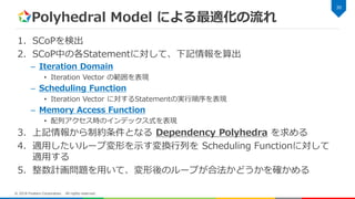
Polyhedral Model による最適化の流れ 1.
SCoPを検出 2. SCoP中の各Statementに対して、下記情報を算出 – Iteration Domain • Iteration Vector の範囲を表現 – Scheduling Function • Iteration Vector に対するStatementの実行順序を表現 – Memory Access Function • 配列アクセス時のインデックス式を表現 3. 上記情報から制約条件となる Dependency Polyhedra を求める 4. 適用したいループ変形を示す変換行列を Scheduling Functionに対して 適用する 5. 整数計画問題を用いて、変形後のループが合法かどうかを確かめる 30 © 2018 Fixstars Corporation. All rights reserved.
32.
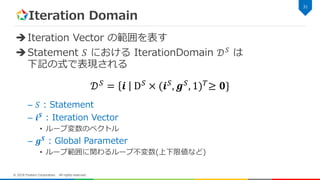
Iteration Domain Iteration Vector
の範囲を表す Statement 𝑆 における IterationDomain 𝒟 𝑆 は 下記の式で表現される – 𝑆 : Statement – 𝒊 𝑺 : Iteration Vector • ループ変数のベクトル – 𝒈 𝑺 : Global Parameter • ループ範囲に関わるループ不変数(上下限値など) 31 © 2018 Fixstars Corporation. All rights reserved. 𝒟 𝑆 = 𝒊 D 𝑆 × (𝒊 𝑆 , 𝒈 𝑆 , 1) 𝑇 ≥ 𝟎}
33.
Iteration Domain の導出例 S1についての導出例 –
Iteration Vector • 𝒊 𝑆1 = (𝑦, 𝑥) – Global Parameter • 𝒈 𝑆1 = (𝐻, 𝑊) – Iteration Vector の範囲 • 0 ≤ 𝑦 < 𝐻 (⇒ 0 ≤ 𝑦 ≤ 𝐻 − 1) • 0 ≤ 𝑥 < 𝑊 (⇒ 0 ≤ 𝑥 ≤ 𝑊 − 1) 32 © 2018 Fixstars Corporation. All rights reserved. サンプルコード for (y=0; y<H; y++) for (x=0; x<W; x++) { S1: s = 0; //S1 for (ky=0; y<KS; ky++) for (kx=0; x<KS; kx++) S2: s += src[y+ky][x+kx] * kernel[ky][kx]; S3: dst[y][x] = s >> t; }
34.
Iteration Domain の導出例 S2についての導出例 –
Iteration Vector • 𝒊 𝑆2 = (𝑦, 𝑥, 𝑘𝑦, 𝑘𝑥) – Global Parameter • 𝒈 𝑆2 = (𝐻, 𝑊, 𝐾𝑆) – Iteration Vector の範囲 • 0 ≤ 𝑦 < 𝐻 (⇒ 0 ≤ 𝑥 ≤ 𝐻 − 1) • 0 ≤ 𝑥 < 𝑊 (⇒ 0 ≤ 𝑦 ≤ 𝑊 − 1) • 0 ≤ 𝑘𝑦 < 𝐾𝐻 (⇒ 0 ≤ 𝑘𝑦 ≤ 𝐾𝐻 − 1) • 0 ≤ 𝑘𝑥 < 𝐾𝑊 (⇒ 0 ≤ 𝑘𝑥 ≤ 𝐾𝑊 − 1) 33 © 2018 Fixstars Corporation. All rights reserved. サンプルコード for (y=0; y<H; y++) for (x=0; x<W; x++) { S1: s = 0; //S1 for (ky=0; y<KS; ky++) for (kx=0; x<KS; kx++) S2: s += src[y+ky][x+kx] * kernel[ky][kx]; S3: dst[y][x] = s >> t; }
35.
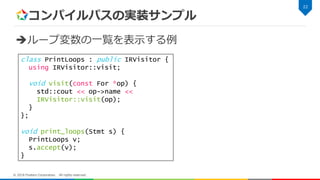
Iteration Domain の導出例 スライドp31を満たす ようにD
𝑆1 を求めると 同様にD 𝑆2 を求めると 34 © 2018 Fixstars Corporation. All rights reserved. 𝒟 𝑆1 = { 𝑦, 𝑥 | 1 0 0 0 0 −1 0 1 0 −1 0 1 0 0 0 0 −1 0 1 −1 𝑦 𝑥 H W 1 ≥ 𝟎} 𝒟 𝑆2 = 𝑦, 𝑥, 𝑘𝑦, 𝑘𝑥 1 0 0 0 0 0 0 0 −1 0 1 0 0 0 0 −1 0 1 0 0 0 0 0 0 0 −1 0 1 0 0 0 −1 0 0 1 0 0 0 0 0 0 0 −1 0 0 0 1 −1 0 0 0 1 0 0 0 0 0 0 0 −1 0 0 0 −1 𝑦 𝑥 𝑘𝑦 𝑘𝑥 H W KS 1 ≥ 𝟎} 𝒟 𝑆1 の領域 サンプルコード for (y=0; y<H; y++) for (x=0; x<W; x++) { S1: s = 0; //S1 for (ky=0; y<KS; ky++) for (kx=0; x<KS; kx++) S2: s += src[y+ky][x+kx] * kernel[ky][kx]; S3: dst[y][x] = s >> t; } O W-1 H-1 y x
36.
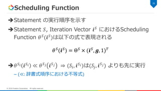
Scheduling Function Statement の実行順序を示す Statement
𝑆, Iteration Vector 𝒊 𝑆 におけるScheduling Function 𝜃 𝑆 (𝒊 𝑆 )は以下の式で表現される 𝜃 𝑆 𝑖 𝒊 𝑆 𝑖 ≪ 𝜃 𝑆 𝑗 𝒊 𝑆 𝑗 ⇒ (𝑆𝑖, 𝒊 𝑆 𝑖)は(𝑆𝑗, 𝒊 𝑆 𝑗) よりも先に実行 – (≪: 辞書式順序における不等式) 35 © 2018 Fixstars Corporation. All rights reserved. 𝜃 𝑆 (𝒊 𝑆 ) = Θ 𝑆 × (𝒊 𝑆 , 𝒈, 1) 𝑇
37.
Scheduling Function の導出方法
SCoPのASTで根から各Statementへ訪問 各Node訪問時にネスト内のStatement番号を付与 – ループ文の場合は更にループ変数を追加 サンプルコードにおける例 36 © 2018 Fixstars Corporation. All rights reserved. S1 y x ky kx S3 S2 0 0 0 1 2 0 0 for (y=0; y<H; y++) for (x=0; x<W; x++) { S1: s = 0; //S1 for (ky=0; ky<KS; ky++) for (kx=0; kx<KS; kx++) S2: s += src[y+ky][x+kx] * kernel[ky][kx]; S3: dst[y][x] = s >> t; } 𝜃 𝑆1 𝑦, 𝑥 = 0, 𝑦, 0, 𝑥, 0 𝑇 𝜃 𝑆2 𝑦, 𝑥, 𝑘𝑦, 𝑘𝑥 = 0, 𝑦, 0, 𝑥, 1, 𝑘𝑦, 0, 𝑘𝑥, 0 𝑇 𝜃 𝑆3 𝑦, 𝑥 = 0, 𝑦 0, 𝑥, 2 𝑇 サンプルコード サンプルコードのAST
38.
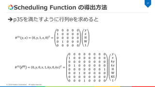
Scheduling Function の導出方法 p35を満たすように行列Θを求めると 37 ©
2018 Fixstars Corporation. All rights reserved. 𝜃 𝑆1 𝑦, 𝑥 = 0, 𝑦, 1, 𝑥, 0 𝑇 = 0 0 0 0 0 1 0 0 0 0 0 0 0 0 0 0 1 0 0 0 0 0 0 0 0 𝑦 𝑥 H W 1 𝜃 𝑆2 𝒊 𝑺𝟐 = 0, 𝑦, 0, 𝑥, 1, 𝑘𝑦, 0, 𝑘𝑥 𝑇 = 0 0 0 0 0 0 0 0 1 0 0 0 0 0 0 0 0 0 0 0 0 0 0 0 0 1 0 0 0 0 0 0 0 0 0 0 0 0 0 1 0 0 1 0 0 0 0 0 0 0 0 0 0 0 0 0 0 0 0 1 0 0 0 0 𝑦 𝑥 𝑘𝑦 𝑘𝑥 H W KS 1
39.
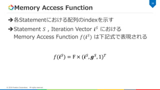
Memory Access Function 各Statementにおける配列のindexを示す Statement
𝑆 , Iteration Vector 𝒊 𝑆 における Memory Access Function 𝑓(𝒊 𝑆 ) は下記式で表現される 38 © 2018 Fixstars Corporation. All rights reserved. 𝑓(𝒊 𝑆 ) = F × (𝒊 𝑆 , 𝒈 𝑆 , 1) 𝑇
40.
Memory Access Function
の導出 39 © 2018 Fixstars Corporation. All rights reserved. 𝑓 𝑆2 𝑠𝑟𝑐 𝑦, 𝑥, 𝑘𝑦, 𝑘𝑥 = 𝑦 + 𝑘𝑦, 𝑥 + 𝑘𝑥 𝑇 = 1 0 1 0 0 0 0 0 0 1 0 1 0 0 0 0 𝑦 𝑥 𝑘𝑦 𝑘𝑥 H W KS 1 𝑓 𝑆3 𝑑𝑠𝑡 𝑦, 𝑥 = 𝑦, 𝑥 𝑇 = 1 0 0 0 0 0 1 0 0 0 𝑦 𝑥 H W 1 サンプルコード for (y=0; y<H; y++) for (x=0; x<W; x++) { S1: s = 0; //S1 for (ky=0; y<KS; ky++) for (kx=0; x<KS; kx++) S2: s += src[y+ky][x+kx] * kernel[ky][kx]; S3: dst[y][x] = s >> t; }
41.
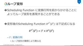
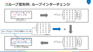
ループ変形 Scheduling Function に変換行列を前からかけることに よってループ変形を表現することができる 変形後のScheduling
Function 𝜃 𝑆′ 𝒊 𝑆 は下記式になる – 𝒯: 変換行列 • ループ変形の種類により異なる 40 © 2018 Fixstars Corporation. All rights reserved. 𝜃 𝑆′ 𝒊 𝑆 = 𝒯 × 𝜃 𝑆 (𝒊 𝑆 )
42.
ループ変形例: ループインターチェンジ 41 © 2018
Fixstars Corporation. All rights reserved. 𝜃 𝑆1 𝑖, 𝑗 = 0 0 0 0 0 1 0 0 0 0 0 0 0 0 0 0 1 0 0 0 0 0 0 0 0 𝑖 𝑗 N M 1 𝜃 𝑆1′ 𝑖, 𝑗 = 0 0 0 0 0 0 𝟏 0 0 0 0 0 0 0 0 𝟏 0 0 0 0 0 0 0 0 0 𝑖 𝑗 N M 1 for (i=0; i<N; i++) for (j=0; j<M; j++) S1(i, j); for (j=0; j<M; j++) for (i=0; i<N; i++) S1(i, j); サンプルコード サンプルコード(変形後) スケジューリング スケジューリング(変形後) 𝒯 = 0 0 0 0 1 0 0 0 1 0 0 0 1 0 0 0 1 0 0 0 1 0 0 0 0 × ループインターチェンジの変換行列 iループとjループが入れ替わっている
43.
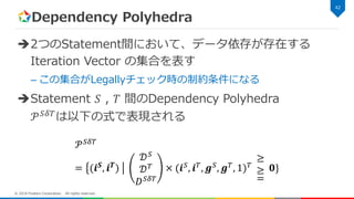
Dependency Polyhedra 2つのStatement間において、データ依存が存在する Iteration Vector
の集合を表す – この集合がLegallyチェック時の制約条件になる Statement 𝑆 , 𝑇 間のDependency Polyhedra 𝒫 𝑆𝛿𝑇 は以下の式で表現される 42 © 2018 Fixstars Corporation. All rights reserved. 𝒫 𝑆𝛿𝑇 = (𝒊 𝑺, 𝒊 𝑻) 𝒟 𝑆 𝒟 𝑇 𝐷 𝑆𝛿𝑇 × (𝒊 𝑆, 𝒊 𝑇, 𝒈 𝑆, 𝒈 𝑇, 1) 𝑇 ≥ ≥ = 𝟎}
44.
Dependency Polyhedra の導出例 1.
SとTのIteration Domainを並べる – SのIteration Domain 43 © 2018 Fixstars Corporation. All rights reserved. Dependency Polyhedra for (i=0; i<N; i++) { S: s[i] = 0; for (j=0; j<M; j++) { T: s[i] = s[i] + a[i][j] * x[j]; } } サンプルコード 𝒫 𝑆𝛿𝑇 = 1 0 0 0 0 0 −1 0 0 1 0 0 0 1 0 0 0 0 0 −1 0 1 0 0 0 0 1 0 0 0 0 0 −1 0 1 0 1 −1 0 0 0 0 𝑖 𝑆 𝑖 𝑇 𝑗 𝑇 𝑁 M 1 ≥ ≥ ≥ ≥ ≥ ≥ = 0
45.
Dependency Polyhedra の導出例 1.
SとTのIteration Domainを並べる – SのIteration Domain – TのIteration Domain 44 © 2018 Fixstars Corporation. All rights reserved. Dependency Polyhedra for (i=0; i<N; i++) { S: s[i] = 0; for (j=0; j<M; j++) { T: s[i] = s[i] + a[i][j] * x[j]; } } サンプルコード 𝒫 𝑆𝛿𝑇 = 1 0 0 0 0 0 −1 0 0 1 0 0 0 1 0 0 0 0 0 −1 0 1 0 0 0 0 1 0 0 0 0 0 −1 0 1 0 1 −1 0 0 0 0 𝑖 𝑆 𝑖 𝑇 𝑗 𝑇 𝑁 M 1 ≥ ≥ ≥ ≥ ≥ ≥ = 0
46.
Dependency Polyhedra の導出例 1.
SとTのIteration Domainを並べる – SのIteration Domain – TのIteration Domain 2. SとT間のMemory Access Functionの等式を作る – 𝑠: 𝑖 𝑆 = 𝑖 𝑇 45 © 2018 Fixstars Corporation. All rights reserved. 𝒫 𝑆𝛿𝑇 = 1 0 0 0 0 0 −1 0 0 1 0 0 0 1 0 0 0 0 0 −1 0 1 0 0 0 0 1 0 0 0 0 0 −1 0 1 0 1 −1 0 0 0 0 𝑖 𝑆 𝑖 𝑇 𝑗 𝑇 𝑁 M 1 ≥ ≥ ≥ ≥ ≥ ≥ = 0 for (i=0; i<N; i++) { S: s[i] = 0; for (j=0; j<M; j++) { T: s[i] = s[i] + a[i][j] * x[j]; } } サンプルコード Dependency Polyhedra
47.
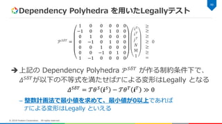
Dependency Polyhedra を用いたLegallyテスト 上記の
Dependency Polyhedra 𝒫 𝑆𝛿𝑇 が作る制約条件下で、 𝛥 𝑆𝛿𝑇 が以下の不等式を満たせば𝒯による変形はLegally となる – 整数計画法で最小値を求めて、最小値が0以上であれば 𝒯による変形はLegally といえる 46 © 2018 Fixstars Corporation. All rights reserved. 𝛥 𝑆𝛿𝑇 = 𝒯𝜃 𝑆 𝒊 𝑆 − 𝒯𝜃 𝑇 𝒊 𝑇 ≫ 0 𝒫 𝑆𝛿𝑇 = 1 0 0 0 0 0 −1 0 0 1 0 0 0 1 0 0 0 0 0 −1 0 1 0 0 0 0 1 0 0 0 0 0 −1 0 1 0 1 −1 0 0 0 0 𝑖 𝑆 𝑖 𝑇 𝑗 𝑇 𝑁 M 1 ≥ ≥ ≥ ≥ ≥ ≥ = 0
48.
HalideコンパイラでPolyhedral Model 47 © 2018
Fixstars Corporation. All rights reserved.
49.
Polyhedral Model 実装概要 実装内容 –
Polyhedral Model解析情報の作成 • Iteration Domain • Scheduling Function • Memory Access Function – 簡単なループ自動並列化モジュール • 依存ベクトルを使って並列化判定 – IP使ってLegallyチェックするところまでは実装出来てません… コード – https://github.com/akmaru/Halide/tree/polyhedral-model 48 © 2018 Fixstars Corporation. All rights reserved.
50.
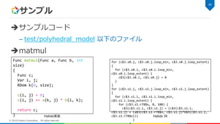
サンプル サンプルコード – test/polyhedral_model 以下のファイル matmul 49 ©
2018 Fixstars Corporation. All rights reserved. Func matmul(Func a, Func b, int size) { Func c; Var i, j; RDom k(0, size); c(i, j) = 0; c(i, j) += a(k, j) * b(i, k); return c; } for (c$3.s0.j, c$3.s0.j.loop_min, c$3.s0.j.loop_extent) { for (c$3.s0.i, c$3.s0.i.loop_min, c$3.s0.i.loop_extent) { c$3(c$3.s0.i, c$3.s0.j) = 0 } } for (c$3.s1.j, c$3.s1.j.loop_min, c$3.s1.j.loop_extent) { for (c$3.s1.i, c$3.s1.i.loop_min, c$3.s1.i.loop_extent) { for (c$3.s1.r78$x, 0, 100) { c$3(c$3.s1.i, c$3.s1.j) = (c$3(c$3.s1.i, c$3.s1.j) + (a$3(c$3.s1.r78$x, c$3.s1.j)*b$3(c$3.s1.i, c$3.s1.r78$x))) } Halide実装 Halide IR
51.
Polyhedral Model 解析情報 50 ©
2018 Fixstars Corporation. All rights reserved. Building polyhedral models... Iteration Sets := (c$3.s0.j, c$3.s0.i) Domain := [c$3.s0.j.loop_min, ((c$3.s0.j.loop_min + c$3.s0.j.loop_extent) + -1)], [c$3.s0.i.loop_min, ((c$3.s0.i.loop_min + c$3.s0.i.loop_extent) + -1)] Schedule := (2, c$3.s0.j, 0, c$3.s0.i, 0) Provides := c$3 := (c$3.s0.i, c$3.s0.j) : (c$3.s0.i, c$3.s0.j) Iteration Sets := (c$3.s1.j, c$3.s1.i, c$3.s1.r78$x) Domain := [c$3.s1.j.loop_min, ((c$3.s1.j.loop_min + c$3.s1.j.loop_extent) + -1)], [c$3.s1.i.loop_min, ((c$3.s1.i.loop_min + c$3.s1.i.loop_extent) + -1)], [0, 99] Schedule := (3, c$3.s1.j, 0, c$3.s1.i, 0, c$3.s1.r78$x, 0) Provides := c$3 := (c$3.s1.i, c$3.s1.j) : (c$3.s1.i, c$3.s1.j) Calls := c$3 := (c$3.s1.i, c$3.s1.j) : (c$3.s1.i, c$3.s1.j) a$3 := (c$3.s1.r78$x, c$3.s1.j) : (c$3.s1.r78$x, c$3.s1.j) b$3 := (c$3.s1.i, c$3.s1.r78$x) : (c$3.s1.i, c$3.s1.r78$x)
52.
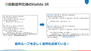
自動並列化後のHalide IR 51 © 2018
Fixstars Corporation. All rights reserved. for (c$3.s0.j, c$3.s0.j.loop_min, c$3.s0.j.loop_extent) { for (c$3.s0.i, c$3.s0.i.loop_min, c$3.s0.i.loop_extent) { c$3(c$3.s0.i, c$3.s0.j) = 0 } } for (c$3.s1.j, c$3.s1.j.loop_min, c$3.s1.j.loop_extent) { for (c$3.s1.i, c$3.s1.i.loop_min, c$3.s1.i.loop_extent) { for (c$3.s1.r78$x, 0, 100) { c$3(c$3.s1.i, c$3.s1.j) = (c$3(c$3.s1.i, c$3.s1.j) + (a$3(c$3.s1.r78$x, c$3.s1.j)*b$3(c$3.s1.i, c$3.s1.r78$x))) } } } parallel (c$3.s0.j, c$3.s0.j.loop_min, c$3.s0.j.loop_extent) { for (c$3.s0.i, c$3.s0.i.loop_min, c$3.s0.i.loop_extent) { c$3(c$3.s0.i, c$3.s0.j) = 0 } } parallel (c$3.s1.j, c$3.s1.j.loop_min, c$3.s1.j.loop_extent) { for (c$3.s1.i, c$3.s1.i.loop_min, c$3.s1.i.loop_extent) { for (c$3.s1.r78$x, 0, 100) { c$3(c$3.s1.i, c$3.s1.j) = (c$3(c$3.s1.i, c$3.s1.j) + (a$3(c$3.s1.r78$x, c$3.s1.j)*b$3(c$3.s1.i, c$3.s1.r78$x))) } } } 最外ループを正しく並列化出来ている! 並列化前のHalide IR 並列化後のHalide IR
53.
Fibonacci関数の例 ループ伝搬依存がある場合… 52 © 2018 Fixstars
Corporation. All rights reserved. Flow依存を正しく検出できている! Building polyhedral models... Iteration Sets := (f.s1.r4$x) Domain := [2, 99] Schedule := (1, f.s1.r4$x, 0) Provides := f := (f.s1.r4$x) : (f.s1.r4$x) Calls := f := ((f.s1.r4$x + -2)) : (f.s1.r4$x) f := ((f.s1.r4$x + -1)) : (f.s1.r4$x) Flow: f(f.s1.r4$x) -> f((f.s1.r4$x + -2)) : (=, -, =) Flow: f(f.s1.r4$x) -> f((f.s1.r4$x + -1)) : (=, -, =) f(x) = x; f(r.x) = f(r.x-2) + f(r.x- 1); for (f.s0.x, f.s0.x.loop_min, f.s0.x.loop_extent) { f(f.s0.x) = f.s0.x } for (f.s1.r4$x, 2, 98) { f(f.s1.r4$x) = (f((f.s1.r4$x + -2)) + f((f.s1.r4$x + -1))) } Halide実装 Halide IR 解析結果
54.
まとめ 53 © 2018 Fixstars
Corporation. All rights reserved.
55.
まとめ Halide – 画像処理の高性能計算に特化したDSL – 短い記述量でアルゴリズム記述が可能 –
最適化の記述が簡単でコードポータビリティも高い Halide IR – データ並列系プログラムを表現する高レベルな中間表現 – コンパイラによる解析や最適化が手軽に行える 54 © 2018 Fixstars Corporation. All rights reserved.
56.
55
Editor's Notes
#6
2012年 MIT
#7
DSLの例: HDL, BNF, Makefile
#14
2016年 カーネギー・メロン大学
#17
Tensor Comprehensions 2018/2/14 Facebook research
#30
PLUTO オハイオ州立大学 Polly LLVM オハイオ州立大学
Download


![Halide[1]
画像処理の高性能計算に特化したドメイン固有言語(DSL)
– http://halide-lang.org/
特徴
– C++の内部DSLとして実装
– アルゴリズムとスケジューリングを分離して記述
• 純粋関数型言語による簡素なアルゴリズム記述
• 計算タイミングと最適化を指定するスケジューリング記述
– 様々なHWターゲットに対する最適化・コード生成が可能
• ターゲット: x86, ARM, POWER, MIPS, NVIDIA GPGPU, Hexagon
• 出力形式: LLVM-IR, C/C++, OpenCL, OpenGL, Matlab, Metal,
4
© 2018 Fixstars Corporation. All rights reserved.
[1] J.Ragan-Kelley, et al, Halide: A Language and Compiler for Optimizing Parallelism, Locality, and Recomputation in Image Processing Pipelines, PLDI 2013](https://image.slidesharecdn.com/preludetohalidepublic-181112031425/85/Prelude-to-Halide-5-320.jpg)

![スケジューリング記述
計算の意味を変えずにコードを変形出来る
– 計算レベルやデータの保持の仕方を指定
• 計算量とメモリアクセスのトレードオフが決定される
– ループ変形
• 並列化、ベクトル化
• アンロール、インターチェンジ、タイリング、
どのようなスケジューリングを適用するかはユーザーが指定する
– 自動で最適化をしてくれるわけではない
– 自動でスケジューリングを適用してくれる機能(Auto Scheduler[1])も
存在する
12
© 2018 Fixstars Corporation. All rights reserved.
[1] R.T.Mullapudi, et al, Automatically Scheduling Halide Image Processing Pipelines, ACM SIGGRAPH 2016](https://image.slidesharecdn.com/preludetohalidepublic-181112031425/85/Prelude-to-Halide-13-320.jpg)
![計算量と使用メモリ量のトレードオフ
13
© 2018 Fixstars Corporation. All rights reserved.
Func blur_x, blur_y;
Var x, y;
blur_x(x, y) = in(x, y) + in(x+1, y);
blur_y(x, y) = (blur_x(x, y) + blur_x(x, y+1))
/ 4;
for (int y=0; y<height; y++) {
for (int x=0; x<width; x++) {
blur_x[y][x] = in[y][x] +
in[y][x+1];
}
}
for (int y=0; y<height; y++) {
for (int x=0; x<width; x++) {
blur_y[y][x] =
(blur_x[y][x] + blur_x[y+1][x])
/ 4;
}
}
for (int y=0; y<height; y++) {
for (int x=0; x<width; x++) {
blur_x[0][x] = in[y][x] +
in[y][x+1];
blur_x[1][x] =
in[y+1][x] + in[y+1][x+1];
}
for (int x=0; x<width; x++) {
blur_y[y][x] =
(blur_x[0][x] + blur_x[1][x]) /
4;
}
}
for (int y=0; y<height; y++) {
for (int x=0; x<width; x++) {
blur_y[y][x] = (in[x][y] +
in[x+1][y] +
in[x][y+1] + in[x+1][y+1]) / 4;
}
}
compute_root
compute_at
compute_inline
計算量小
使用メモリ量小
アルゴリズム記述](https://image.slidesharecdn.com/preludetohalidepublic-181112031425/85/Prelude-to-Halide-14-320.jpg)


![Iteration Domain の導出例
S1についての導出例
– Iteration Vector
• 𝒊 𝑆1 = (𝑦, 𝑥)
– Global Parameter
• 𝒈 𝑆1
= (𝐻, 𝑊)
– Iteration Vector の範囲
• 0 ≤ 𝑦 < 𝐻 (⇒ 0 ≤ 𝑦 ≤ 𝐻 − 1)
• 0 ≤ 𝑥 < 𝑊 (⇒ 0 ≤ 𝑥 ≤ 𝑊 − 1)
32
© 2018 Fixstars Corporation. All rights reserved.
サンプルコード
for (y=0; y<H; y++)
for (x=0; x<W; x++) {
S1: s = 0; //S1
for (ky=0; y<KS; ky++)
for (kx=0; x<KS; kx++)
S2: s += src[y+ky][x+kx] *
kernel[ky][kx];
S3: dst[y][x] = s >> t;
}](https://image.slidesharecdn.com/preludetohalidepublic-181112031425/85/Prelude-to-Halide-33-320.jpg)
![Iteration Domain の導出例
S2についての導出例
– Iteration Vector
• 𝒊 𝑆2 = (𝑦, 𝑥, 𝑘𝑦, 𝑘𝑥)
– Global Parameter
• 𝒈 𝑆2
= (𝐻, 𝑊, 𝐾𝑆)
– Iteration Vector の範囲
• 0 ≤ 𝑦 < 𝐻 (⇒ 0 ≤ 𝑥 ≤ 𝐻 − 1)
• 0 ≤ 𝑥 < 𝑊 (⇒ 0 ≤ 𝑦 ≤ 𝑊 − 1)
• 0 ≤ 𝑘𝑦 < 𝐾𝐻 (⇒ 0 ≤ 𝑘𝑦 ≤ 𝐾𝐻 − 1)
• 0 ≤ 𝑘𝑥 < 𝐾𝑊 (⇒ 0 ≤ 𝑘𝑥 ≤ 𝐾𝑊 − 1)
33
© 2018 Fixstars Corporation. All rights reserved.
サンプルコード
for (y=0; y<H; y++)
for (x=0; x<W; x++) {
S1: s = 0; //S1
for (ky=0; y<KS; ky++)
for (kx=0; x<KS; kx++)
S2: s += src[y+ky][x+kx] *
kernel[ky][kx];
S3: dst[y][x] = s >> t;
}](https://image.slidesharecdn.com/preludetohalidepublic-181112031425/85/Prelude-to-Halide-34-320.jpg)
![Iteration Domain の導出例
スライドp31を満たす
ようにD 𝑆1
を求めると
同様にD 𝑆2
を求めると
34
© 2018 Fixstars Corporation. All rights reserved.
𝒟 𝑆1 = { 𝑦, 𝑥 |
1 0 0 0 0
−1 0 1 0 −1
0 1 0 0 0
0 −1 0 1 −1
𝑦
𝑥
H
W
1
≥ 𝟎}
𝒟 𝑆2
= 𝑦, 𝑥, 𝑘𝑦, 𝑘𝑥
1 0 0 0 0 0 0 0
−1 0 1 0 0 0 0 −1
0 1 0 0 0 0 0 0
0 −1 0 1 0 0 0 −1
0 0 1 0 0 0 0 0
0 0 −1 0 0 0 1 −1
0 0 0 1 0 0 0 0
0 0 0 −1 0 0 0 −1
𝑦
𝑥
𝑘𝑦
𝑘𝑥
H
W
KS
1
≥ 𝟎}
𝒟 𝑆1
の領域
サンプルコード
for (y=0; y<H; y++)
for (x=0; x<W; x++) {
S1: s = 0; //S1
for (ky=0; y<KS; ky++)
for (kx=0; x<KS; kx++)
S2: s += src[y+ky][x+kx] *
kernel[ky][kx];
S3: dst[y][x] = s >> t;
}
O W-1
H-1
y
x](https://image.slidesharecdn.com/preludetohalidepublic-181112031425/85/Prelude-to-Halide-35-320.jpg)
![Scheduling Function の導出方法
SCoPのASTで根から各Statementへ訪問
各Node訪問時にネスト内のStatement番号を付与
– ループ文の場合は更にループ変数を追加
サンプルコードにおける例
36
© 2018 Fixstars Corporation. All rights reserved.
S1
y
x
ky
kx
S3
S2
0
0
0 1 2
0
0
for (y=0; y<H; y++)
for (x=0; x<W; x++) {
S1: s = 0; //S1
for (ky=0; ky<KS; ky++)
for (kx=0; kx<KS; kx++)
S2: s += src[y+ky][x+kx] *
kernel[ky][kx];
S3: dst[y][x] = s >> t;
}
𝜃 𝑆1 𝑦, 𝑥 = 0, 𝑦, 0, 𝑥, 0 𝑇
𝜃 𝑆2
𝑦, 𝑥, 𝑘𝑦, 𝑘𝑥 = 0, 𝑦, 0, 𝑥, 1, 𝑘𝑦, 0, 𝑘𝑥, 0 𝑇
𝜃 𝑆3 𝑦, 𝑥 = 0, 𝑦 0, 𝑥, 2 𝑇
サンプルコード
サンプルコードのAST](https://image.slidesharecdn.com/preludetohalidepublic-181112031425/85/Prelude-to-Halide-37-320.jpg)
![Memory Access Function の導出
39
© 2018 Fixstars Corporation. All rights reserved.
𝑓 𝑆2 𝑠𝑟𝑐 𝑦, 𝑥, 𝑘𝑦, 𝑘𝑥 = 𝑦 + 𝑘𝑦, 𝑥 + 𝑘𝑥 𝑇 =
1 0 1 0 0 0 0 0
0 1 0 1 0 0 0 0
𝑦
𝑥
𝑘𝑦
𝑘𝑥
H
W
KS
1
𝑓 𝑆3 𝑑𝑠𝑡 𝑦, 𝑥 = 𝑦, 𝑥 𝑇
=
1 0 0 0 0
0 1 0 0 0
𝑦
𝑥
H
W
1
サンプルコード
for (y=0; y<H; y++)
for (x=0; x<W; x++) {
S1: s = 0; //S1
for (ky=0; y<KS; ky++)
for (kx=0; x<KS; kx++)
S2: s += src[y+ky][x+kx] * kernel[ky][kx];
S3: dst[y][x] = s >> t;
}](https://image.slidesharecdn.com/preludetohalidepublic-181112031425/85/Prelude-to-Halide-40-320.jpg)
![Dependency Polyhedra の導出例
1. SとTのIteration Domainを並べる
– SのIteration Domain
43
© 2018 Fixstars Corporation. All rights reserved.
Dependency Polyhedra
for (i=0; i<N; i++) {
S: s[i] = 0;
for (j=0; j<M; j++) {
T: s[i] = s[i] + a[i][j] *
x[j];
}
}
サンプルコード
𝒫 𝑆𝛿𝑇 =
1 0 0 0 0 0
−1 0 0 1 0 0
0 1 0 0 0 0
0 −1 0 1 0 0
0 0 1 0 0 0
0 0 −1 0 1 0
1 −1 0 0 0 0
𝑖 𝑆
𝑖 𝑇
𝑗 𝑇
𝑁
M
1
≥
≥
≥
≥
≥
≥
=
0](https://image.slidesharecdn.com/preludetohalidepublic-181112031425/85/Prelude-to-Halide-44-320.jpg)
![Dependency Polyhedra の導出例
1. SとTのIteration Domainを並べる
– SのIteration Domain
– TのIteration Domain
44
© 2018 Fixstars Corporation. All rights reserved.
Dependency Polyhedra
for (i=0; i<N; i++) {
S: s[i] = 0;
for (j=0; j<M; j++) {
T: s[i] = s[i] + a[i][j] *
x[j];
}
}
サンプルコード
𝒫 𝑆𝛿𝑇 =
1 0 0 0 0 0
−1 0 0 1 0 0
0 1 0 0 0 0
0 −1 0 1 0 0
0 0 1 0 0 0
0 0 −1 0 1 0
1 −1 0 0 0 0
𝑖 𝑆
𝑖 𝑇
𝑗 𝑇
𝑁
M
1
≥
≥
≥
≥
≥
≥
=
0](https://image.slidesharecdn.com/preludetohalidepublic-181112031425/85/Prelude-to-Halide-45-320.jpg)
![Dependency Polyhedra の導出例
1. SとTのIteration Domainを並べる
– SのIteration Domain
– TのIteration Domain
2. SとT間のMemory Access Functionの等式を作る
– 𝑠: 𝑖 𝑆 = 𝑖 𝑇
45
© 2018 Fixstars Corporation. All rights reserved.
𝒫 𝑆𝛿𝑇 =
1 0 0 0 0 0
−1 0 0 1 0 0
0 1 0 0 0 0
0 −1 0 1 0 0
0 0 1 0 0 0
0 0 −1 0 1 0
1 −1 0 0 0 0
𝑖 𝑆
𝑖 𝑇
𝑗 𝑇
𝑁
M
1
≥
≥
≥
≥
≥
≥
=
0
for (i=0; i<N; i++) {
S: s[i] = 0;
for (j=0; j<M; j++) {
T: s[i] = s[i] + a[i][j] *
x[j];
}
}
サンプルコード
Dependency Polyhedra](https://image.slidesharecdn.com/preludetohalidepublic-181112031425/85/Prelude-to-Halide-46-320.jpg)

![Polyhedral Model 解析情報
50
© 2018 Fixstars Corporation. All rights reserved.
Building polyhedral models...
Iteration Sets := (c$3.s0.j, c$3.s0.i)
Domain := [c$3.s0.j.loop_min, ((c$3.s0.j.loop_min + c$3.s0.j.loop_extent) + -1)],
[c$3.s0.i.loop_min, ((c$3.s0.i.loop_min + c$3.s0.i.loop_extent) + -1)]
Schedule := (2, c$3.s0.j, 0, c$3.s0.i, 0)
Provides :=
c$3 := (c$3.s0.i, c$3.s0.j) : (c$3.s0.i, c$3.s0.j)
Iteration Sets := (c$3.s1.j, c$3.s1.i, c$3.s1.r78$x)
Domain := [c$3.s1.j.loop_min, ((c$3.s1.j.loop_min + c$3.s1.j.loop_extent) + -1)],
[c$3.s1.i.loop_min, ((c$3.s1.i.loop_min + c$3.s1.i.loop_extent) + -1)], [0, 99]
Schedule := (3, c$3.s1.j, 0, c$3.s1.i, 0, c$3.s1.r78$x, 0)
Provides :=
c$3 := (c$3.s1.i, c$3.s1.j) : (c$3.s1.i, c$3.s1.j)
Calls :=
c$3 := (c$3.s1.i, c$3.s1.j) : (c$3.s1.i, c$3.s1.j)
a$3 := (c$3.s1.r78$x, c$3.s1.j) : (c$3.s1.r78$x, c$3.s1.j)
b$3 := (c$3.s1.i, c$3.s1.r78$x) : (c$3.s1.i, c$3.s1.r78$x)](https://image.slidesharecdn.com/preludetohalidepublic-181112031425/85/Prelude-to-Halide-51-320.jpg)
![Fibonacci関数の例
ループ伝搬依存がある場合…
52
© 2018 Fixstars Corporation. All rights reserved.
Flow依存を正しく検出できている!
Building polyhedral models...
Iteration Sets := (f.s1.r4$x)
Domain := [2, 99]
Schedule := (1, f.s1.r4$x, 0)
Provides :=
f := (f.s1.r4$x) : (f.s1.r4$x)
Calls :=
f := ((f.s1.r4$x + -2)) : (f.s1.r4$x)
f := ((f.s1.r4$x + -1)) : (f.s1.r4$x)
Flow: f(f.s1.r4$x) -> f((f.s1.r4$x + -2)) : (=,
-, =)
Flow: f(f.s1.r4$x) -> f((f.s1.r4$x + -1)) : (=,
-, =)
f(x) = x;
f(r.x) = f(r.x-2) + f(r.x-
1);
for (f.s0.x, f.s0.x.loop_min, f.s0.x.loop_extent) {
f(f.s0.x) = f.s0.x
}
for (f.s1.r4$x, 2, 98) {
f(f.s1.r4$x) = (f((f.s1.r4$x + -2)) + f((f.s1.r4$x +
-1)))
}
Halide実装
Halide IR
解析結果](https://image.slidesharecdn.com/preludetohalidepublic-181112031425/85/Prelude-to-Halide-53-320.jpg)


![[Basic 13] 型推論 / 最適化とコード出力](https://cdn.slidesharecdn.com/ss_thumbnails/basic-13-180314083351-thumbnail.jpg?width=640&height=640&fit=bounds)

