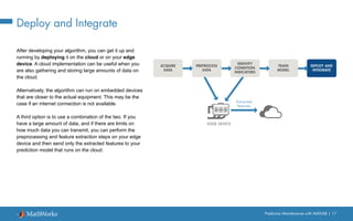
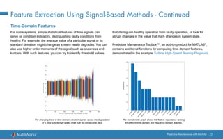
The document outlines the concept and implementation of predictive maintenance using MATLAB, emphasizing its advantages over reactive and preventive maintenance by allowing for the estimation of machine failure times. It details the workflow for developing predictive maintenance algorithms, including data acquisition, preprocessing, and training machine learning models based on extracted condition indicators. The process aims to enhance machine reliability, minimize downtime, and optimize maintenance scheduling while utilizing diverse data sources and advanced analytical techniques.


![Predictive Maintenance with MATLAB | 44
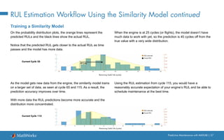
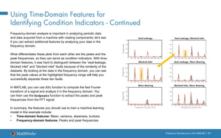
One of the goals of predictive maintenance is to estimate the
remaining useful life (RUL) of a system. RUL is the time between a
system’s current condition and failure. Depending on your system,
time can be represented in terms of days, flights, cycles, or any other
quantity.
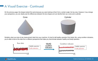
On the plot, we see the deterioration path of a machine over time.
This ebook explores three common models used to estimate RUL
(similarity, survival, and degradation) and then walks through the RUL
workflow with an example using a similarity model.
What Is Remaining Useful Life?
Time
Machine deterioration profile
Remaining useful life (RUL)
Current condition
Failure condition
[ Number of days ]
[ Miles ]
[ Cycles ]
…
Condition
indicator](https://image.slidesharecdn.com/predictive-maintenance-ebook-all-chapters-250123211349-acd47a13/85/predictive-maintenance-ebook-all-chapters-pdf-44-320.jpg)