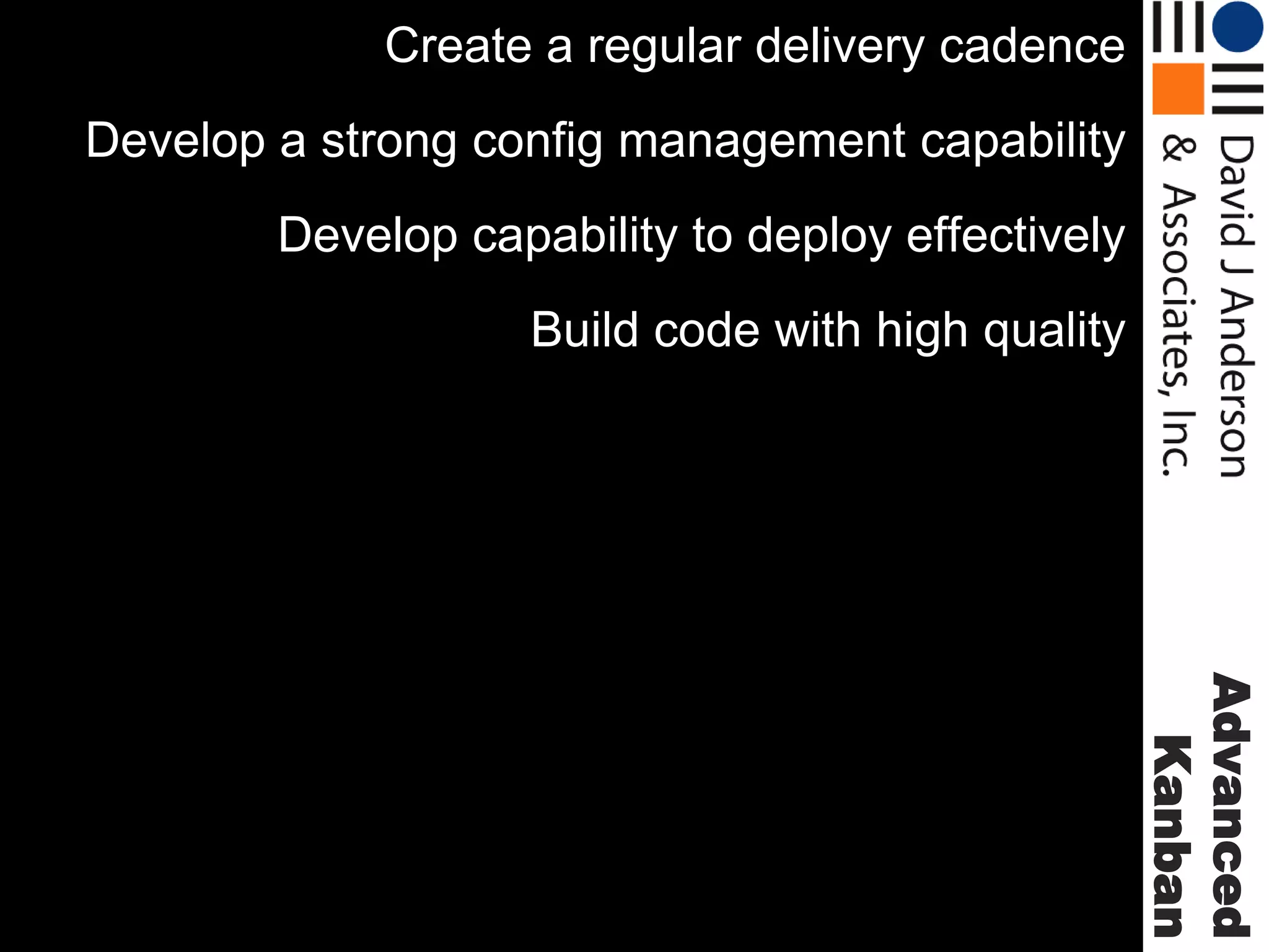
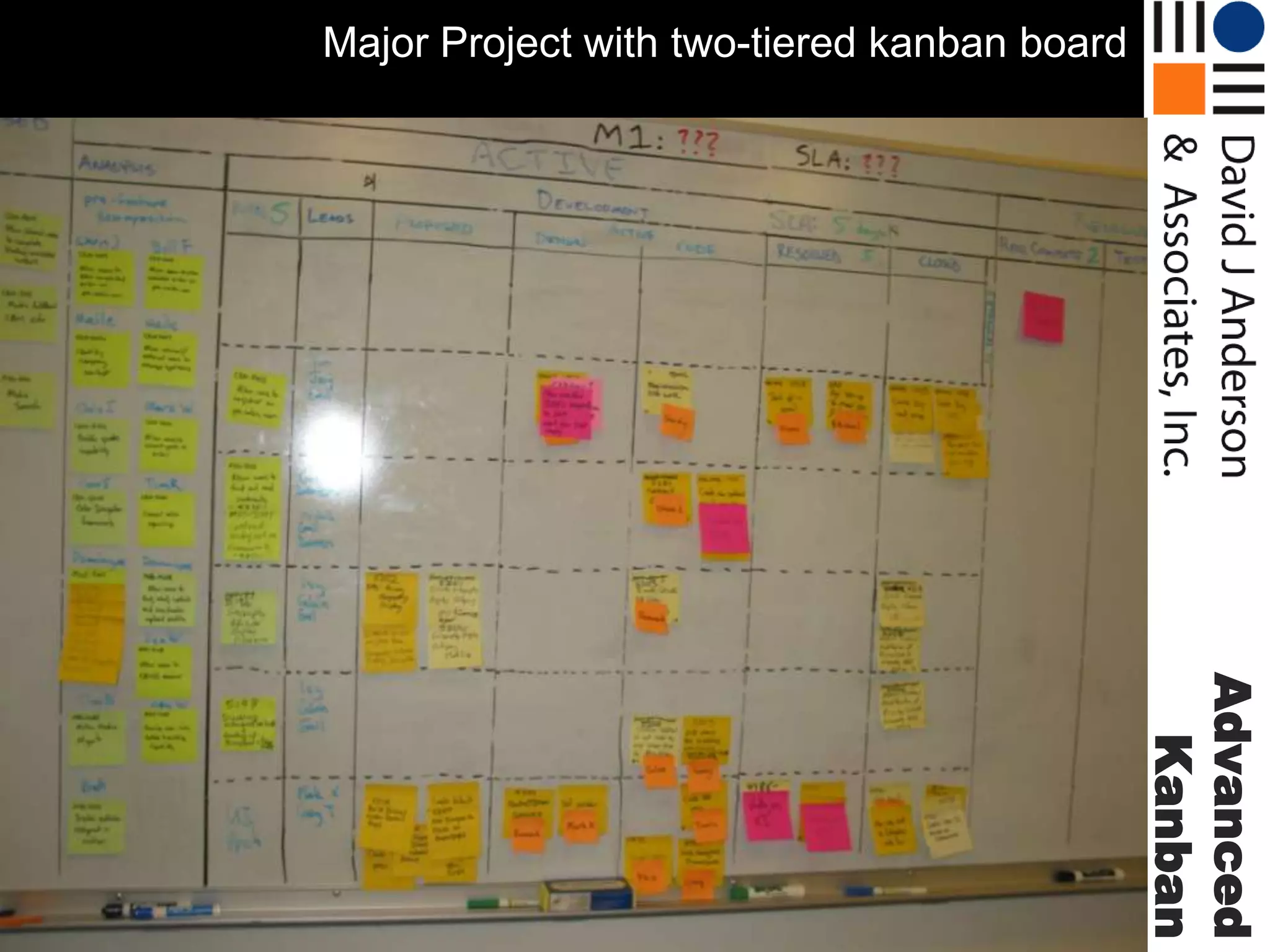
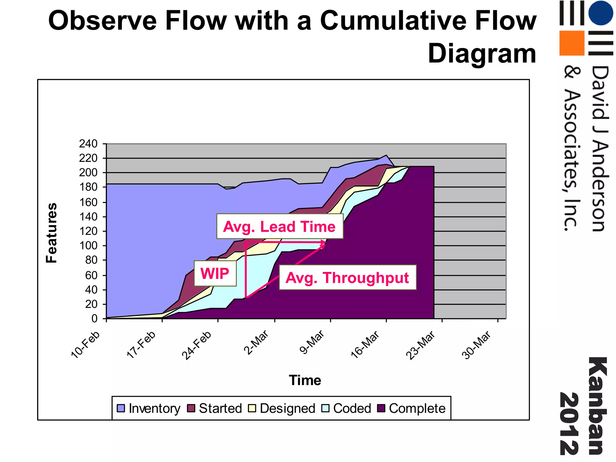
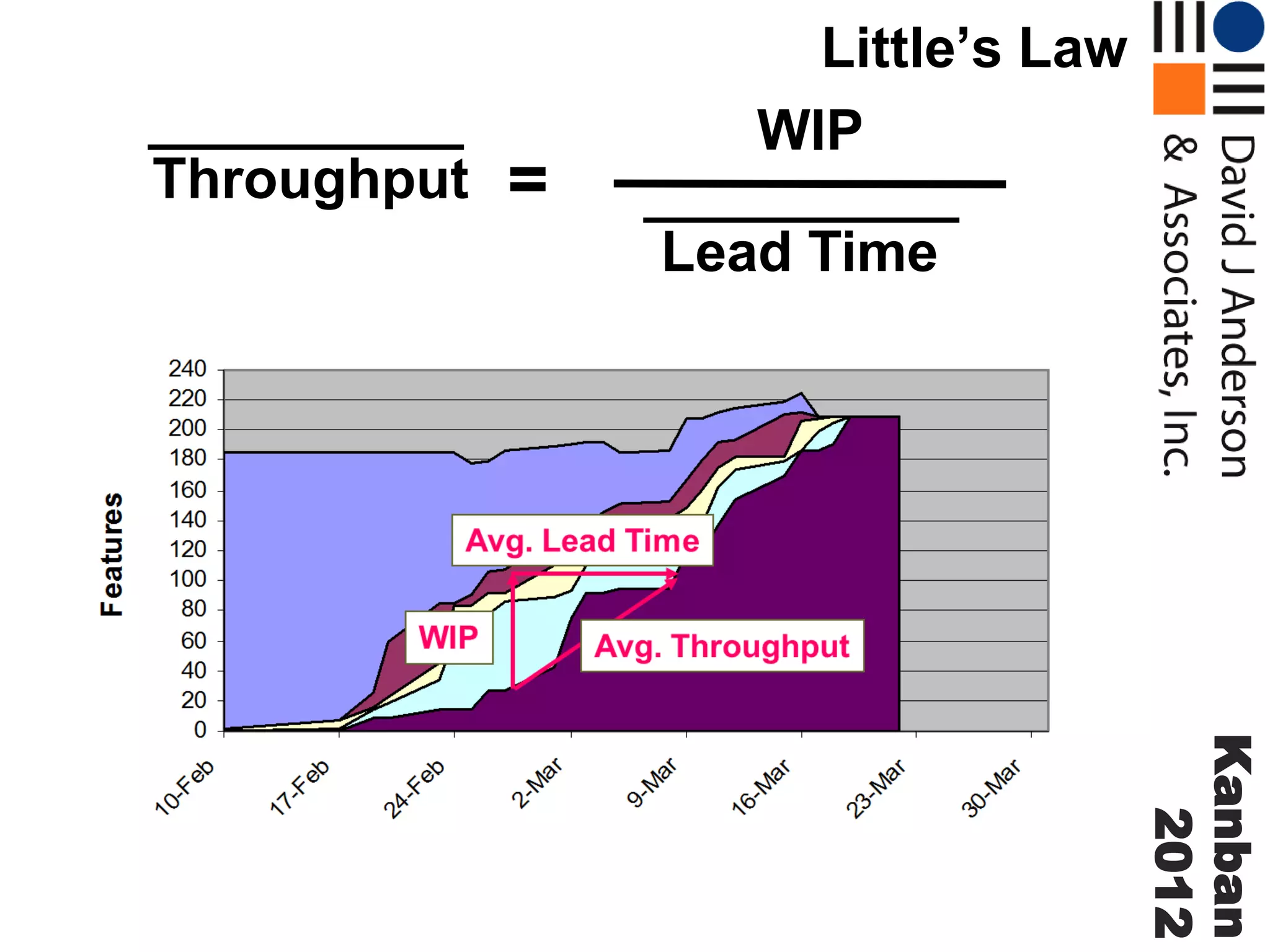
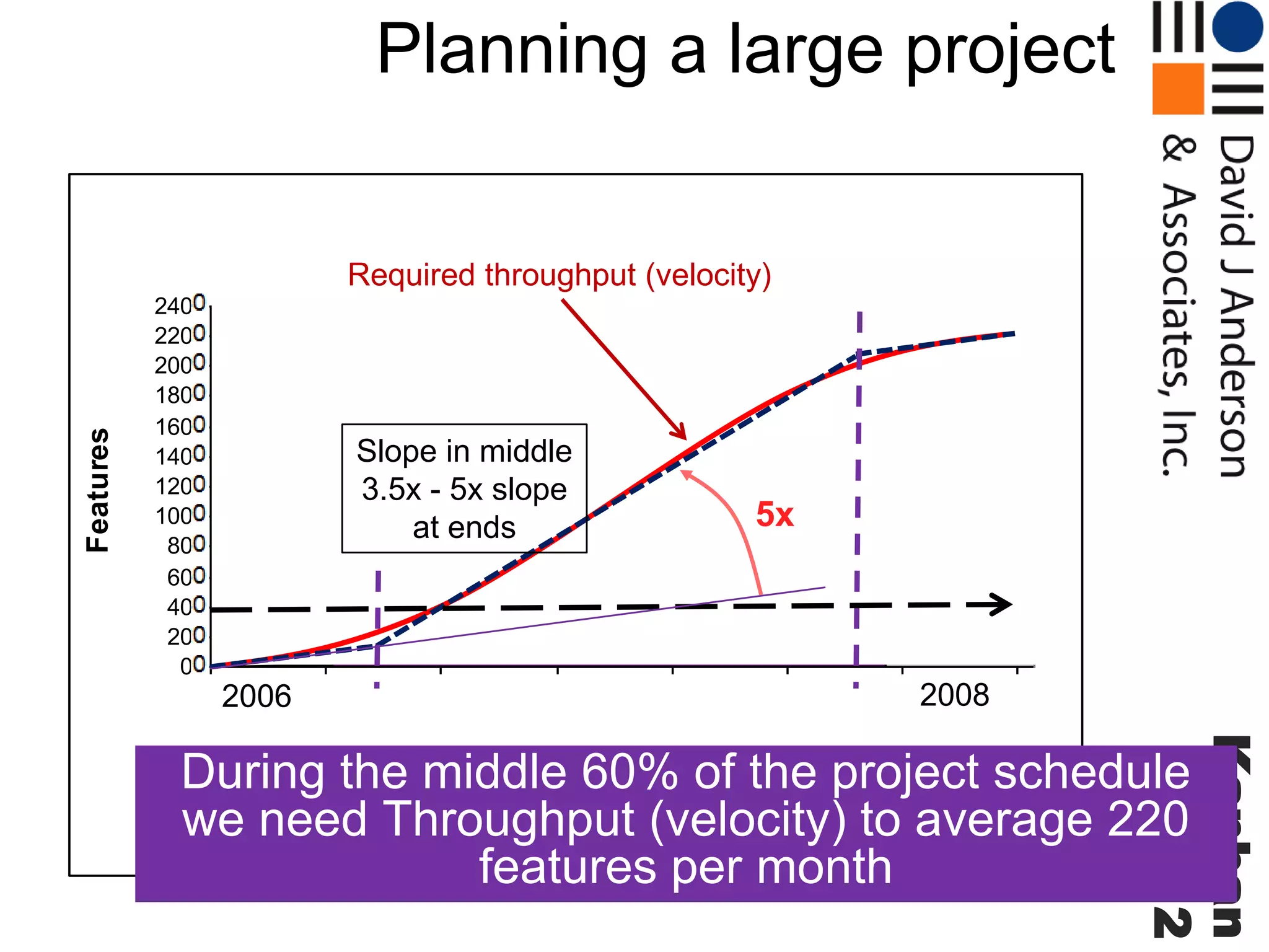
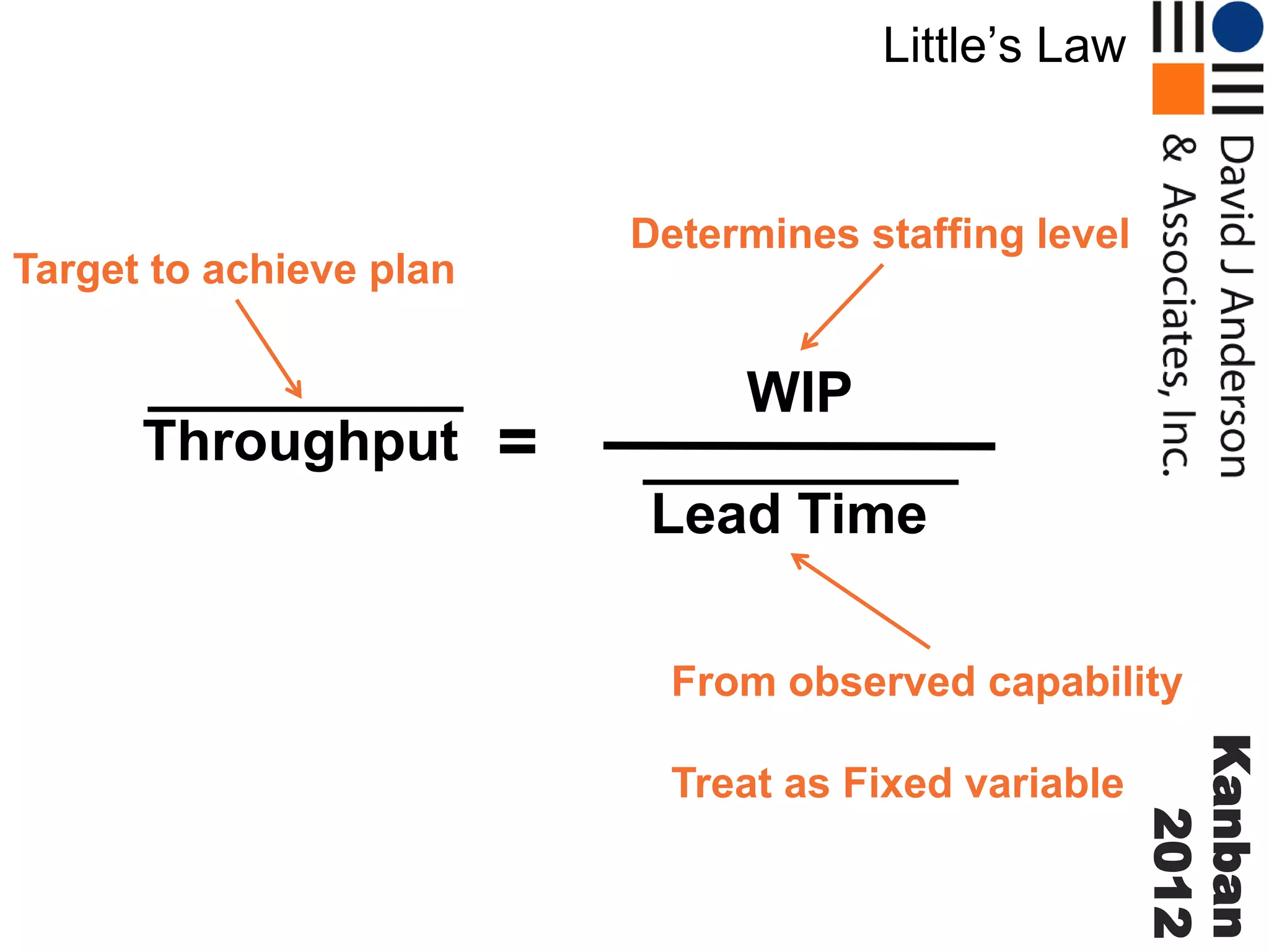
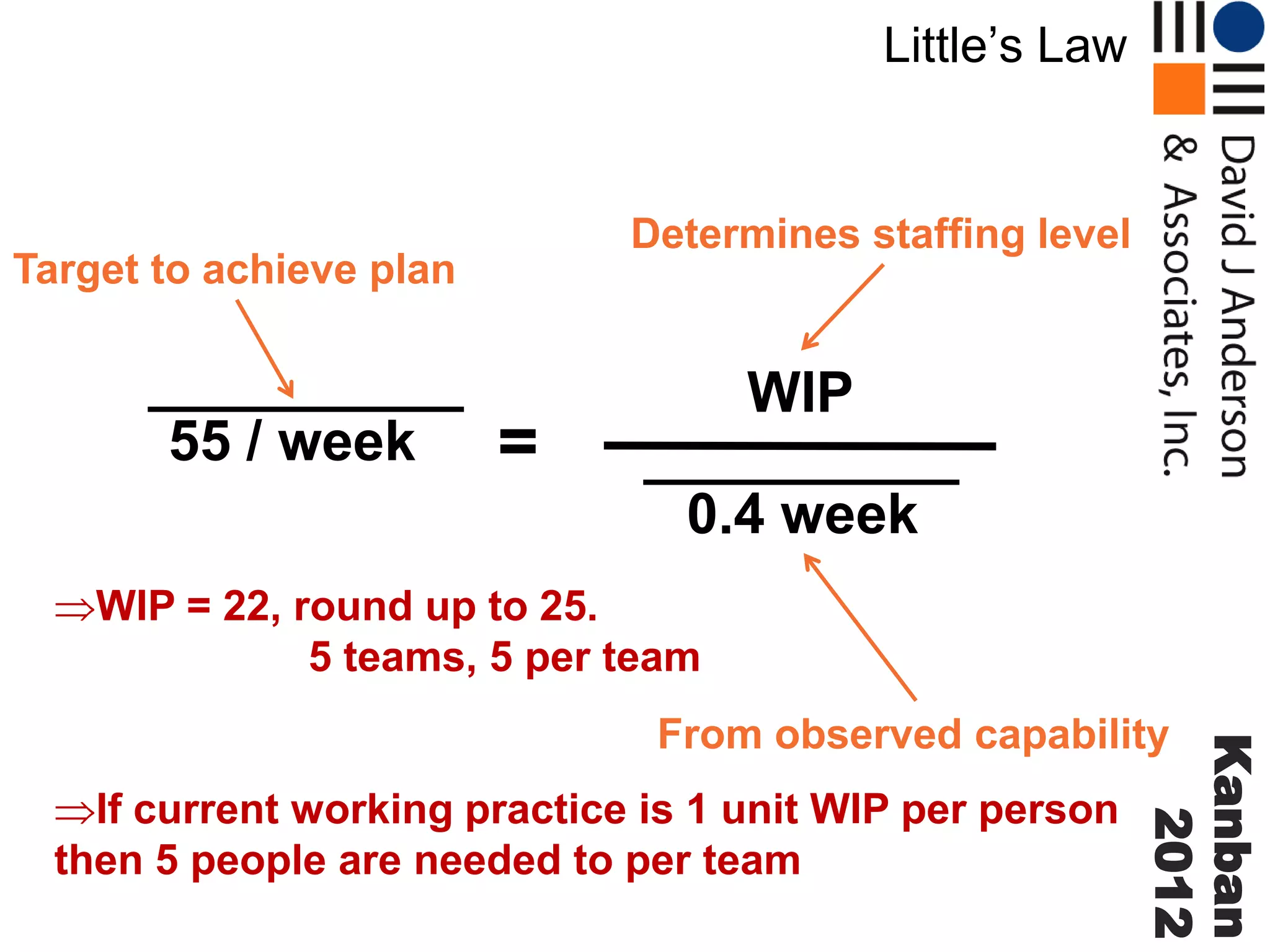
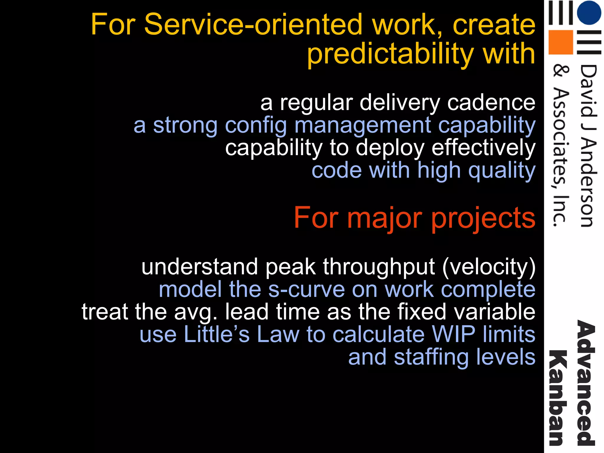
Metrics, measurement, probabilistic forecasting and setting expectations to enable predictable delivery with Kanban. Track session from OOP 2012 Munich

1. Predictability & Measurement
with Kanban
OOP 2012
Munich
January 2012
Twitter: agilemanager
David J. Anderson
David J. Anderson & Associates
Email: dja@djaa.com

2. Book Published
April 2010
Available from
djaa.com
Advanced
Kanban
A 72,000 word
intro to the topic

3. German
published January, 2011
Kanban
2012
Translation by
Arne Roock &
Henning Wolf
of IT-Agile

4. http://leankanbanuniversity.com
http://www.limitedwipsociety.org
LinkedIn Groups: Software Kanban
Yahoo! Groups: kanbandev
Yahoo! Groups: kanbanops

5. Delivering predictability with
Kanban
requires some different techniques
for different types of work such as
software maintenance and support
or
Advanced
Kanban
major project work

6. Service-oriented work
Advanced
Kanban

7. Create a regular delivery cadence
Develop a strong config management capability
Develop capability to deploy effectively
Build code with high quality
Advanced
Kanban

8. Understand capability by studying the natural
philosophy of the work
MARCH
Lead Time Distribution
2.5
# CRs
2
1.5
1
0.5
106
101
96
91
86
81
76
71
66
61
56
51
46
41
36
31
26
21
16
11
6
1
0
Days
Lead Time Distribution
APRIL
3.5
Majority of CRs range 30 -> 55
2
Outliers
1.5
1
0.5
Days
8
14
1
14
4
13
0
3
6
7
12
12
11
10
99
92
85
78
71
64
57
50
43
36
29
22
15
8
0
1
CRs & Bugs
2.5
Advanced
Kanban
3

9. Observe Flow with a spectral analysis histogram
of lead time
Lead Time Distribution
3.5
3
CRs & Bugs
2.5
2
1.5
1
0.5
1
4
7
0
3
6
8
14
14
13
12
12
11
10
99
92
85
78
71
64
57
50
43
36
29
22
8
15
1
0
Days
SLA expectation of
44 days with 85% on-time
Advanced
Kanban
Mean of
31 days
SLA expectation of
51 days with 98% on-time

10. 44 or 51 days will not be good enough for some
feature requests, so offer a package of classes of
service
Advanced
Kanban

11. Package of Classes with SLAs

As soon as possible


100% on-time


providing 24 days advance notice
Up to 51 days

98% on-time guarantee
Up to 51 days

50% on-time
Advanced
Kanban

Full transparency

12. Lead time
Standard Class Items
Fixed Date Items
Advanced
Kanban
Expedite Item
Features Delivered

13. Allocate capacity across classes of service in
order to deliver against anticipated demand
5
4
Analysis
Input
Queue In Prog Done
3
4
Development
Dev
Ready In Prog Done
2
Build
Ready
2 = 20 total
Test
Release
Ready
...
Allocation
4 = 20%
10 = 50%
6 = 30%
Advanced
Kanban
+1 = +5%

14. Major Project Work
Advanced
Kanban

15. Requires all the same underlying
data as used in service oriented
work
plus
Advanced
Kanban

16. Major Project with two-tiered kanban board
Advanced
Kanban

17. Observe Flow with a Cumulative Flow
Diagram
Avg. Lead Time
Time
Inventory
Started
Designed
Coded
Complete
30
-M
ar
23
-M
ar
16
-M
ar
9M
ar
2M
ar
eb
Avg. Throughput
Kanban
2012
24
-F
eb
WIP
17
-F
eb
240
220
200
180
160
140
120
100
80
60
40
20
0
10
-F
Features
Device Management Ike II Cumulative Flow

18. Throughput
=
Little’s Law
WIP
Lead Time
Kanban
2012

19. Cumulative Flow and
Predictive Modeling with S-Curve
Inventory
Started
Designed
Coded
Complete
30
-M
ar
23
-M
ar
16
-M
ar
9M
ar
2M
ar
eb
Time
Kanban
2012
24
-F
eb
Typical S-curve
17
-F
eb
240
220
200
180
160
140
120
100
80
60
40
20
0
10
-F
Features
Device Management Ike II Cumulative Flow

20. Simulating S-Curve with a Z
60%
Slope in middle
3.5x - 5x slope
at ends
5x
20%
Time
Inventory
Started
Designed
Coded
Complete
30
-M
ar
23
-M
ar
16
-M
ar
9M
ar
2M
ar
eb
24
-F
eb
20%
Kanban
2012
17
-F
eb
240
220
200
180
160
140
120
100
80
60
40
20
0
10
-F
Features
Device Management Ike II Cumulative Flow

21. Track actual throughput against projection
Inventory
Started
Designed
Coded
Complete
30
-M
ar
23
-M
ar
16
-M
ar
9M
ar
2M
ar
eb
Time
Kanban
2012
24
-F
eb
Track delta between
planned and actual
each day
17
-F
eb
240
220
200
180
160
140
120
100
80
60
40
20
0
10
-F
Features
Device Management Ike II Cumulative Flow

22. Unplanned Work Report
Scope Creep
Dark Matter
Advanced
Kanban

23. Planning a large project
Device Management Ike II Cumulative Flow
2008
30
-M
ar
23
-M
ar
16
-M
ar
9M
ar
2M
ar
5x
Kanban
2012
24
-F
eb
2006
eb
Slope in middle
3.5x - 5x slope
at ends
17
-F
eb
240
220
200
180
160
140
120
100
80
60
40
20
0
10
-F
Features
Required throughput (velocity)
During the middle 60% of the project schedule
Time
we need Throughput (velocity) to average 220
Inventory Started Designed Coded Complete
features per month

24. Little’s Law
Determines staffing level
Target to achieve plan
Throughput
=
WIP
Lead Time
From observed capability
Kanban
2012
Treat as Fixed variable

25. Changing the WIP limit without
maintaining the staffing level ratio
represents a change to the way of
working. It is a change to the
system design. And will produce a
change in the observed ‘common
cause’ capability of the system
Kanban
2012

26. Plan based on currently observed
capability and current working
practices. Do not assume process
improvements.
If changing WIP to reduce
undesirable effects (e.g.
multitasking), get new sample data
(perform a spike) to observe the
new capability
Kanban
2012

27. Little’s Law
Determines staffing level
Target to achieve plan
55 / week
WIP
=
0.4 week
WIP = 22, round up to 25.
5 teams, 5 per team
If current working practice is 1 unit WIP per person
then 5 people are needed to per team
Kanban
2012
From observed capability

28. Conclusions
Advanced
Kanban

29. For Service-oriented work, create
predictability with
a regular delivery cadence
a strong config management capability
capability to deploy effectively
code with high quality
For major projects
Advanced
Kanban
understand peak throughput (velocity)
model the s-curve on work complete
treat the avg. lead time as the fixed variable
use Little’s Law to calculate WIP limits
and staffing levels

30. Thank you!
Advanced
Kanban
dja@djaa.com
http://djaa.com/

31. About…
David Anderson is a thought leader in
managing effective software teams. He leads
a consulting, training and publishing
business dedicated to developing,
promoting and implementing sustainable
evolutionary approaches for management of
knowledge workers.
He has 30 years experience in the high
technology industry starting with computer
games in the early 1980’s. He has led software
teams delivering superior productivity and
quality using innovative agile methods at large
companies such as Sprint and Motorola.
David is a founder of the Lean Kanban
University, a business dedicated to assuring
quality of training in Lean and Kanban
throughout the world.
http://leankanbanuniversity.com
Email: dja@djaa.com Twitter: agilemanager
Advanced
Kanban
David is the author of two books, Agile
Management for Software Engineering –
Applying the Theory of Constraints for Business
Results, and Kanban – Successful Evolutionary
Change for your Technology Business.