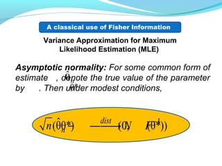
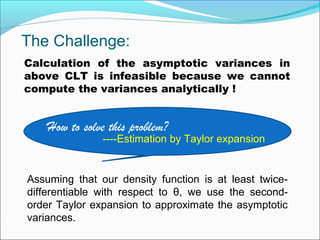
- The document compares two methods for approximating Fisher information in the scalar case: sums of products of derivatives and the negative sum of second derivatives. - For independent and identically distributed random variables, the asymptotic variances of the two methods can be estimated using Taylor expansions. Conditions are derived under which the second derivative method is more accurate. 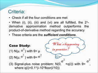- For a case study with normal distributions, the conditions are met, showing the second derivative method outperforms the product of derivatives method. The analysis provides theoretical justification for commonly using the second derivative approximation.

1. Analysis of Data-Based
Methods for Approximating
Fisher Information in the
Scalar Case
Shenghan Guo
Applied Math & Statistics, Johns Hopkins University

2. Bulletin:
Conclusion

3. Problem Setting:
Random variables with density function p(z|θ),
where the unknown parameter θ is scalar. Fisher information
is the measurement of information amount carried by z
regarding θ. 2
(θ) (θ| )nF E g =  z
[ ](θ) (θ| ) ,nF E H=− z
where
log ( |θ)
(θ| )
θ
p
g
∂
=
∂
z
z
and 2
2
log ( |θ)
(θ| )
θ
p
H
∂
=
∂
z
z
1 2[ , ,..., ]T
nZ Z Z=z

4. Applications:

5. Variance Approximation for Maximum
Likelihood Estimation (MLE)
Asymptotic normality: For some common form of
estimate , denote the true value of the parameter
by . Then under modest conditions,
ˆθn
A classical use of Fisher Information
θ*
1ˆ(θθ*) (0, (θ*))
dist
nn N F−
− →

6. A Fact ：
It is difficult to get the true value of Fisher Information in
practice because direct calculation could be difficult, or
we don’t have the explicit forms of the gradient or the
Hessian. Thus approximation is needed.
Typical situations where approximation is
needed:
• State-space models with nuisance parameters (Spall,
J. C. and Garner, J. P. 1990)
• Non-i.i.d. projectile measurements and quantiles (Spall,
J. C. and Maryak, J. L. 1992)
• Inverse heat condition problems (Favennec, Y. 2007)

7. • The unavailability of the true Fisher information in
many practical cases makes a useful approximation
method for this quantity important.
• No prior studies have compared the approximation
methods for Fisher information to decide which one is
more accurate.
• The convention of utilizing the certain approximation
method (e.g. 2nd
-derivative approximation to estimate
Fisher information in the scalar case) needs
theoretical support.
Motivation:

8. Two Methods to Approximate Fisher
Information Number:
I. Sums of Products of Derivatives:
II. Negative Sum of 2nd
Derivative:
2
1
1
(θ) (θ| )
n
n i i
i
G g z
n =
= ∑
1
1
(θ) (θ| )
n
n i i
i
H H z
n =
= − ∑
The reality: Mostly people tend to use the 2nd
derivative method instead of the product-of-
derivatives method, which is more of a convention
without valid theoretical support.

9. My Way to Solve This Question:

10. By the Central Limit Theorem:
Let and , for independent and
identically distributed random variables:
( ) ( )dist 2
(θ) (θ) 0,var ( )n in G F n N g z − →  
( ) [ ]( )dist
(θ) (θ) 0,var ( )n in H F n N H z− →
2 2
( ) (θ| )g g• = • ( ) (θ| )H H• = •
nG
nH
We wonder which one of the estimates and
is more accurate !

11. For independent and non-identically distributed
random variables:
( ) ( )dist
(θ) (θ) 0,n gn G F n N V− →
( ) ( )dist
(θ) (θ) 0,n Hn H F n N V−  →
1 2
1
lim var ( )
n
g i iin
V n g z−
=→∞
 =  ∑where
and [ ]1
1
lim var ( )
n
H i iin
V n H z−
=→∞
= ∑

12. The Challenge:
Calculation of the asymptotic variances in
above CLT is infeasible because we cannot
compute the variances analytically !
How to solve this problem?
----Estimation by Taylor expansion
Assuming that our density function is at least twice-
differentiable with respect to θ, we use the second-
order Taylor expansion to approximate the asymptotic
variances.

13. 2
var ( )ig z 
 
Take expectation of the Taylor expansion
for the product of g(zi)

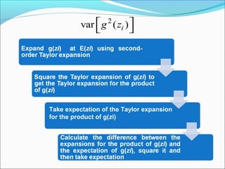
14. [ ]var ( )iH z
Take expectation of the Taylor expansion
for H(zi)
Calculate the difference between the
expansions of H(zi) and the expectation of it,
square it and then take expectation

15. Comparison:
a.Calculate the difference between the asymptotic
variances:
b.To see which method is more accurate, the following
conditions can be checked for the i.i.d. case
(conditions for i.n.i.d. case is provided in the paper):
(i)
(ii)
(iii)
(vi) has the same sign with
[ ]2
var ( ) var ( ) ( )i i g Hg z H z or V V  − − 
2 2
2
4 (μ) (μ) (μ) 0i i i i i ig g H   ′ ′− ≥
   
22 21
(μ) (μ) (μ) (μ) 0
4
i i i i i i i ig g g H
    ′ ′′ ′′+ − ≥ ÷    
(μ) (μ) 0g g′′ ≥
( )2
[ (μ)] (μ) (μ)i i i i i ig g g′ ′′+
6 2 4
(μ)σ(μ)i i i i iE z E z   − − −   

16. Criteria:
• Check if all the four conditions are met
• When (i), (ii), (iii) and (vi) are all fulfilled, the 2nd
-
derivative approximation method outperforms the
product-of-derivative method regarding the accuracy
• These criteria are the sufficient conditions.
Case Study:
(1) N(μ, ) with θ= μ
(2) N(μ, ) with θ=
(3) Signal-plus noise problem: N(0, +q(i)) with θ= ,
where q(i)=0.1*(i-10*floor(i/10))
What’s happening
in practice?2
σ
2
σ 2
σ
2
σ2
σ

17. 3.1188e+08 3.6371 3.1812e-08
1.9226e+08 2.0632 1.9380e-08
1.6222 1.7628 3.3915
2 2
μ1,σ0.1= = 2 2
μ5,σ10= =2
μ0,σ1= =
2
var ( )g z 
 
p-value 7.7846e-05 3.2146e-05 9.4938e-05
2 2
μ1,σ0.1= = 2
μ0,σ1= = 2 2
μ5,σ10= =
[ ]var ( )H z
[ ]2
var ( ) var ( )g z H z 
 
Selected Numerical Results:
Case 2: [ ]2 8 1
var ( ) var ( ) 3 (2σ) 0g z H z −  − = • > 

18. Case Study 3:
6.1060e+07 1.0349 3.5680e-08
2.5194e+07 0.6584 2.0023e-08
2.783 1.5718 1.7820
p-value 0.0269 0.0025 2.3863e-07
[ ]2
var ( ) var ( )i ig z H z 
 
[ ]var ( )iH z
2
var ( )ig z 
 
2 2
σ0.1= 2
σ1 = 2 2
σ10=
2 2
σ0.1= 2
σ1 = 2 2
σ10=
[ ] 1002 1 2 4
1
var ( ) var ( ) 3 (200) (σ) 0i i ii
g z H z q− −
=
  − = • + >  ∑

19. Conclusions:
• We decide which one of the product of derivative
approximation and the 2nd
-order derivative
approximation, is more accurate based on criteria (i),
(ii), (iii) and (vi) for the i.i.d. case
• Similar criteria for the i.n.i.d. scenario exists, which
can be found in the full paper
• For the normal density functions we considered in
our case study, we show that the Hessian methods
outperforms the gradient based method !
Thank you for listening !

20. References:
[1] Guo, S. (2014), "Comparison of Accuracy for Methods to
Approximate Fisher Information in the Scalar Case," M. S. project final
report, Department of Applied Mathematics and Statistics, Johns
Hopkins Univ.; available at arXiv: http://arxiv.org/abs/1501.00218.
[2] Guo, S. (2015), “Analysis of Data-Based Methods for
Approximating Fisher Information in the Scalar Case,” Proceedings of
the 49th Annual Conference on Information Sciences and
Systems, 18−20 March 2015, Baltimore, MD.
submitted to Proceedings of the 49th Annual Conference on Information Sciences and Systems, 18−20 March 2015, Baltimore, MD.

21. ( )
2
22 2 2 2 2
4 4 2 2 3
2 4
var ( )
4 (μ)[ (μ)]σ[ (μ)] (μ) (μ) var (μ)
1
[ (μ)] var (μ) [ (μ)] [ (μ)] var (μ)
16
4 (μ)[ (μ)] (μ) (μ)
i
i
i i
i
g z
g g g g g z
g z g g z
g g g E z
 
 
 ′ ′ ′′≈ + + − 
   ′′ ′ ′′+ − + −   
 ′ ′′+ − 
( )( )2 2 6 2 41
[ (μ)] [ (μ)] (μ) (μ) (μ)σ(μ)
2
i ig g g g E z E z   ′′ ′ ′′+ + − − −   
[ ] [ ] [ ]2 22 21
var ( ) (μ)σ(μ) var (μ)
4
i iH z H H z ′ ′′≈ + − 
i.i.d. case:
2
μ( ),σvar( )i iE z z= =Define and let ( |θ) ( ), ( |θ) ( )g g H H• = • • = •
Consider the symmetric density family:

22. i.n.i.d. case:
( )
2
1
2 2
2 2 2 2
1 1
4 4 2 2 3
1 1
2
var ( )
4 (μ) (μ)σ[ (μ)] (μ) (μ) var (μ)
1
[ (μ)] var (μ) [ (μ)] [ (μ)] var (μ)
16
4 (μ)[ (μ)] (μ) (
n
i i
i
n n
i i i i i i i i i i i i i
i i
n n
i i i i i i i i i i
i i
i i i i i i
g z
g g g g g z
g z g g z
g g g E
=
= =
= =
 
 
 ′ ′ ′′  ≈ + + −  
′′ ′ ′′   + − + −   
′ ′′+
∑
∑ ∑
∑ ∑
( )( )
4
1
2 2 6 2 4
1
μ)
1
[ (μ)] [ (μ)] (μ) (μ) (μ)σ(μ)
2
n
i i
i
n
i i i i i i i i i i i i i
i
z
g g g g E z E z
=
=
 − 
′′ ′ ′′    + + − − −   
∑
∑
[ ]
2 2
2 2
1 1 1
1
var ( ) (μ)σ(μ) var (μ)
4
n n n
i i i i i i i i i
i i i
H z H H z
= = =
   ′ ′′  ≈ + −    ∑ ∑ ∑
Define and let
2
μ( ),σvar( )i i i iE z z= = ( |θ) ( ), ( |θ) ( )i i i ig g H H• = • • = •