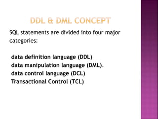
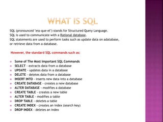
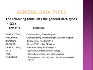
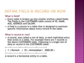
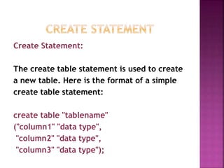
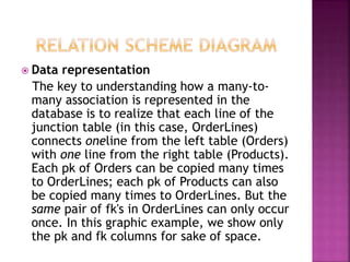
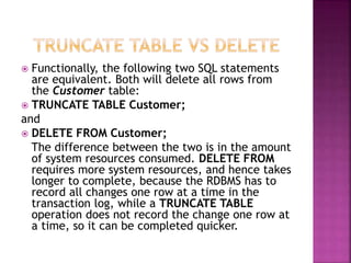
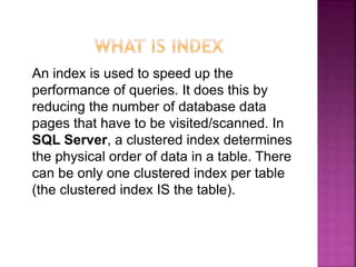
This document provides an overview of relational databases, highlighting their superiority over flat file databases in terms of data management, including advantages such as avoiding data duplication, ensuring data consistency, and facilitating easier data updates. It explains the structure of data in relational databases through tables, fields, and records and introduces SQL as a language used to perform database operations. The document also covers SQL commands, data types, and the importance of primary keys in maintaining unique records.

1. For Beginner

2. Basic knowledge of Flat files and Rational data base:
 A database is a collection of data, which is organized into files
called tables. These tables provide a systematic way of accessing,
managing, and updating data. A relational database is one that
contains multiple tables of data that relate to each other through
special key fields. Relational databases are far more flexible
(though harder to design and maintain) than what are known as
flat file databases, which contain a single table of data.
 To understand the advantages of a relational database, imagine
the needs of two small companies that take customer orders for
their products. Company A uses a flat file database with a single
table named orders to record orders they receive, while Company
B uses a relational database with two tables: orders and
customers.

3.  When a customer places an order with Company A, a
new record (or row) in the table orders is created.
Because Company A has only one table of data, all the
information pertaining to that order must be put into a
single record. This means that the customer's general
information, such as name and address, is stored in
the same record as the order information, such as
product description, quantity, and price. If customers
place more than one order, their general information
will need to be re-entered and thus duplicated for each
order they place.
 Whenever there is duplicate data, as in the case
above, many inconsistencies may arise when users try
to query the database. Additionally, a customer's
change of address would require the database
manager to find all records in orders that the customer
placed, and change the address data for each one.

4.  Company B is much better off with its relational
database. Each of its customers has one and only
one record of general information stored in the
table customers. Each customer's record is
identified by a unique customer code which will
serve as the relational key. When a customer
orders from Company B, the record in orders
need contain only a reference to the customer's
code, because all of the customer's general
information is already stored in customers.
 This approach to entering data solves the
problems of duplicate data and making changes
to customer information. The database manager
need change only one record in customers if
someone changes addresses.

5. Understanding of DATA MANAGEMENT SYSTEM
 An RDBMS (Relational Database Management System) is
essentially a database management system that is
designed to store data which can later be used for a
specific application. The term “RDBMS” stands for the
actual database, which typically comes associated with a
variety of supporting functions and software including SQL
Queries and System Restores. In short, these databases are
an excellent way to store information which will later need
to be retrieved.
 They usually contain more than a single table, and similar
to a spreadsheet, will contain columns and rows that are
used to sort information. From here, data can be deleted,
updated, or inserted. With that being said, let’s take a
look at some steps that you can follow to
successfully BIULD A RELATIONAL DATABASE and “insert”
new information into it.

7. DIAGRAM:

8. Summary - advantages of a relational database
over flat file
 Avoids data duplication
 Avoids inconsistent records
 Easier to change data
 Easier to change data format
 Data can be added and removed easily
 Easier to maintain security.

9. Splitting data into a number of related tables brings many
advantages over a flat file database. These include:
1. Data is only stored once. In the previous example, the city data
was gathered into one table so now there is only one record per
city. The advantages of this are No multiple record changes
needed
More efficient storage Simple to delete or modify details.
All records in other tables having a link to that entry will show
the change
2. Complex queries can be carried out. A language called SQL has
been developed to allow programmers to 'Insert', 'Update',
'Delete', 'Create', 'Drop' table records. These actions are further
refined by a 'Where' clause.
For example
SELECT * FROM Customer WHERE ID = 2
This SQL statement will extract record number 2 from the Customer
table. Far more complicated queries can be written that can
extract data from many tables at once.

10. 3. Better security.
By splitting data into tables, certain tables can be
made confidential. When a person logs on with their
username and password, the system can then limit
access only to those tables whose records they are
authorized to view. For example, a receptionist
would be able to view employee location and contact
details but not their salary. A salesman may see his
team's sales performance but not competing teams.
4. Cater for future requirements.
By having data held in separate tables, it is simple to
add records that are not yet needed but may be in
the future. For example, the city table could be
expanded to include every city and town in the
country, even though no other records are using them
all as yet. A flat file database cannot do this.

11. SQL statements are divided into four major
categories:
data definition language (DDL)
data manipulation language (DML).
data control language (DCL)
Transactional Control (TCL)

12.  Data Definition Language (DDL) statements are
used to define the database structure or
schema.
Some examples:
 CREATE - to create objects in the database
 ALTER - alters the structure of the database
 DROP - delete objects from the database
 TRUNCATE - remove all records from a table,
including all spaces allocated for the records are
removed
 COMMENT - add comments to the data dictionary
 RENAME - rename an object

13. Data Manipulation Language (DML) statements are
used for managing data within schema objects.
Some examples:
 SELECT - retrieve data from the a database
 INSERT - insert data into a table
 UPDATE - updates existing data within a table
 DELETE - deletes all records from a table, the
space for the records remain
 MERGE - UPSERT operation (insert or update)
 CALL - call a PL/SQL or Java subprogram
 EXPLAIN PLAN - explain access path to data
 LOCK TABLE - control concurrency

14. Data Control Language (DCL) statements.
Some examples:
 GRANT - gives user's access privileges to
database
 REVOKE - withdraw access privileges given
with the GRANT command

15.  Transaction Control (TCL) statements are used
to manage the changes made by DML statements.
It allows statements to be grouped together into
logical transactions.
 COMMIT - save work done
 SAVEPOINT - identify a point in a transaction to
which you can later roll back
 ROLLBACK - restore database to original since
the last COMMIT
 SET TRANSACTION - Change transaction options
like isolation level and what rollback segment to
use

16. SQL (pronounced "ess-que-el") stands for Structured Query Language.
SQL is used to communicate with a Rational database.
SQL statements are used to perform tasks such as update data on adatabase,
or retrieve data from a database.
However, the standard SQL commands such as:
 Some of The Most Important SQL Commands
 SELECT - extracts data from a database
 UPDATE - updates data in a database
 DELETE - deletes data from a database
 INSERT INTO - inserts new data into a database
 CREATE DATABASE - creates a new database
 ALTER DATABASE - modifies a database
 CREATE TABLE - creates a new table
 ALTER TABLE - modifies a table
 DROP TABLE - deletes a table
 CREATE INDEX - creates an index (search key)
 DROP INDEX - deletes an index

17. A relational database system contains one or
more objects called tables. The data or
information for the database are stored in
these tables. Tables are uniquely identified by
their names and are comprised of columns and
rows. Columns contain the column name,
data type, and any other attributes for the
column. Rows contain the records or data for
the columns.

18. SQL is just an interface which helps you
communicate with your system’s database
using queries. We rotate our car’s steering
wheel without bothering about what
mechanical reaction might have taken place
in our wheel’s axle. We are only concerned
about turning our car. Similarly when we use
SQL, we only have to fire simple queries to
retrieve data from your database without
thinking about internal database operations.

19. Here is a sample table called "weather".
city, state, high, and low are the columns. The
rows contain the data for this table: Weather
city state high low
Germantown Maryland 105 90
Gaithersburg Maryland 101 92
Rockville Maryland 88 69
San Diego California 77 60
Albuquerque New Mexico 80 72

20. SQL Language elements
 The SQL language is based on several elements. For the convenience
of SQL developers all necessary language commands in the
corresponding DATABASE MANAGEMENT SYSTEM are usually executed
through a specific SQL command-line interface (CLI).
 Clauses - the clauses are components of the statements and the
queries
 Expressions - the expressions can produce scalar values or tables,
which consist of columns and rows of data
 Predicates - they specify conditions, which are used to limit the
effects of the statements and the queries, or to change the program
flow
 Queries - a query will retrieve data, based on a given criteria
 Statements - with the statements one can control transactions,
program flow, connections, sessions, or diagnostics. In database
systems the SQL statements are used for sending queries from a client
SERVER processes the SQL statements and returns replies to the client
program. This allows users to execute a wide range of amazingly fast
data manipulation operations from simple data inputs to complicated
queries.

21. SQL queries
 The SQL queries are the most common and
essential SQL operations. Via an SQL query, one
can search the database for the information
needed. SQL queries are executed with the
“SELECT” statement. An SQL query can be more
specific, with the help of several clauses:
 FROM - it indicates the TABLE where the search
will be made.
 WHERE - it's used to define the rows, in which
the search will be carried. All rows, for which
the WHERE clause is not true, will be excluded.
 ORDER BY - this is the only way to sort the
results in SQL. Otherwise, they will be returned
in a random order.

22. SQL data control, definition and manipulation
 SQL is a language designed to store data, but the data
stored in an SQL database is not static. It can be modified
at any time with the use of several very simple commands.
The SQL syntax is pretty much self explanatory, which
makes it much easier to read and understand.
SQL data manipulation
 Data manipulation is essential for SQL tables - it allows you
to modify an already created table with new information,
update the already existing values or delete them.
 With the INSERT statement, you can add new rows to an
already existing table. New rows can contain information
from the start, or can be with a NULL value.

23. Here are the most common Data types:
 char(size) Fixed-length character string. Size is
specified in parenthesis. Max 255 bytes.
 varchar(size) Variable-length character
string. Max size is specified in parenthesis.
 number(size) Number value with a max
number of column digits specified in
parenthesis.
 date Date value
 number(size,d) Number value with a maximum number of
digits of "size" total, with a maximum number of "d" digits to the right of
the decimal.

24. The following table lists the general data types
in SQL:
DATA TYPE Description
CHARACTER(n) Character string. Fixed-length n
VARCHAR(n) Character string. Variable length.Maximum length n
BINARY(n) Binary string. Fixed-length n
BOOLEAN Stores TRUE or FALSE values
CHARACTER(n) Character string. Fixed-length n
DATE Stores year, month, and day values
TIME Stores hour, minute, and second values
TIMESTAMP Stores year, month, day, hour, minute, and second
values

25. What is table?
 The data in RDBMS is stored in database
objects called tables. The table is a
collection of related data entries and it
consists of columns and rows.
 Remember, a table is the most common and
simplest form of data storage in a relational
database.

26. Following is the example of a CUSTOMERS table:
+----+----------+-----+---------+----------+
| ID | NAME | AGE | ADDRESS | SALARY |
+----+----------+-----+-----------+----------+
| 1 | JOHN | 32 | Ahmedabad | 2000.00 |
| 2 | KOHL | 25 | Delhi | 1500.00 |
| 3 | JJKHAN | 23 | Kota | 2000.00 |
| 4 | URKAN | 25 | Mumbai | 6500.00 |
| 5 | JOE | 27 | Bhopal | 8500.00 |
| 6 | HARRY | 22 | MP | 4500.00 |
+----+----------+-----+-----------+----------+

27.  To create a new table, enter the keywords create
table followed by the table name, followed by an
open parenthesis, followed by the first column name,
followed by the data type for that column, followed
by any optional constraints, and followed by a closing
parenthesis. It is important to make sure you use an
open parenthesis before the beginning table, and a
closing parenthesis after the end of the last column
definition. Make sure you separate each column
definition with a comma. All SQL statements should
end with a ";".
 The table and column names must start with a letter
and can be followed by letters, numbers, or
underscores - not to exceed a total of 30 characters
in length. Do not use any SQL reserved keywords as
names for tables or column names (such as "select",
"create", "insert", etc).

28. What is field?
 Every table is broken up into smaller entities called fields.
The fields in the CUSTOMERS table consist of ID, NAME,
AGE, ADDRESS and SALARY.
 A field is a column in a table that is designed to maintain
specific information about every record in the table.
What is record or row?
 A record, also called a row of data, is each individual entry
that exists in a table. For example there are 7 records in
the above CUSTOMERS table. Following is a single row of
data or record in the CUSTOMERS table:
+----+----------+-----+-----------+----------+
| 1 | Ramesh | 32 | Ahmedabad | 2000.00 |
+----+----------+-----+-----------+----------+
A record is a horizontal entity in a table.

29. What is column?
 A column is a vertical entity in a table that contains all
information associated with a specific field in a table.
 For example, a column in the CUSTOMERS table is ADDRESS,
which represents location description and would consist of the
following:
+-----------+
| ADDRESS |
+-----------+
| Ahmedabad |
| Delhi |
| Kota |
| Mumbai |
| Bhopal |
| MP |
| Indore |
+----+------+

30. What is NULL value?
 A NULL value in a table is a value in a field
that appears to be blank, which means a
field with a NULL value is a field with no
value.
 It is very important to understand that a
NULL value is different than a zero value or a
field that contains spaces. A field with a
NULL value is one that has been left blank
during record creation.

31. SQL Aggregate Functions:
 SQL aggregate functions return a single value,
calculated from values in a column.
Useful aggregate functions:
 AVG() - Returns the average value
 COUNT() - Returns the number of rows
 FIRST() - Returns the first value
 LAST() - Returns the last value
 MAX() - Returns the largest value
 MIN() - Returns the smallest value
 SUM() - Returns the sum

32. Create Statement:
The create table statement is used to create
a new table. Here is the format of a simple
create table statement:
create table "tablename"
("column1" "data type",
"column2" "data type",
"column3" "data type");

33.  To create a new table, enter the keywords create
table followed by the table name, followed by an
open parenthesis, followed by the first column name,
followed by the data type for that column, followed
by any optional constraints, and followed by a closing
parenthesis. It is important to make sure you use an
open parenthesis before the beginning table, and a
closing parenthesis after the end of the last column
definition. Make sure you separate each column
definition with a comma. All SQL statements should
end with a ";".
 The table and column names must start with a letter
and can be followed by letters, numbers, or
underscores - not to exceed a total of 30 characters
in length. Do not use any SQL reserved keywords as
names for tables or column names (such as "select",
"create", "insert", etc).

34.  Example:
create table employee
(first varchar(15),
last varchar(20),
age number (3),
address varchar(30),
city varchar(20),
state varchar(20));
Semicolon after SQL Statements?
 Some database systems require a semicolon at the end of each
SQL statement.
 Semicolon is the standard way to separate each SQL statement
in database systems that allow more than
 one SQL statement to be executed in the same call to the
server

35. Customer Table:
CREATE TABLE customers
( customer_id number(10) NOT NULL,
customer_name varchar2(50) NOT NULL,
address varchar2(50),
city varchar2(50),
state varchar2(25),
zip_code varchar2(10),
CONSTRAINT customers_pk PRIMARY KEY
(customer_id)
customer ID should be the primary key for the
table

36. What is a primary key in Oracle?
 In Oracle, a primary key is a single field or combination of
fields that distinctively defines a record. None of the fields
that are part of the primary key can contain a null value. A
table can have only one primary key.
 Note
 In Oracle, a primary key cannot contain more than 32
columns.A primary key can be defined in either a CREATE
TABLE statement or an ALTER TABLE statement.
 A value of NULL indicates that the value is unknown. A value of
NULL is different from an empty or zero value. No two null
values are equal. Comparisons between two null values, or
between a NULL and any other value, return unknown because
the value of each NULL is unknown.
 Null values generally indicate data that is unknown, not
applicable, or that the data will be added later. For example, a
customer's middle initial may not be known at the time the
customer places an order.


37.  Representing data in rows
 Each real-world individual of a class (for example,
each customer who does business with our enterprise)
is represented by a row of information in a database
table. The row is defined in the relational model as a
tuple that is constructed over a given scheme.
Mathematically, the tuple is a function that assigns a
constant value from the attribute domain to each
attribute of the scheme. Notice that because the
scheme is a set of attributes, we could show them in
any order without changing the meaning of the data in
the row (tuple).


38.  A database table is simply a collection of
zero or more rows. This follows from the
relational model definition of a relation as a
set of tuples over the same scheme. (The
name “relational model” comes from the
relation being the central object in this
model.)

39.  Since each row in a table must be unique, no two rows can have
exactly the same values for every one of their attributes.
Therefore, there must be some set of attributes (it might be the
set of all attributes) in each relation whose values, taken
together, guarantee uniqueness of each row. Any set of attributes
that can do this is called a super key (SK). Super keys are a
property of the relation (table), filled in with any reasonable set
of real-world data, even though we show them in the relation
scheme drawing for convenience.
 The database designer picks one of the possible super key
attribute sets to serve as the primary key (PK) of the relation.
(Notice that the PK is an SK, but not all SKs are PKs!) The PK is
sometimes also called a unique identifier for each row of the
table. This is not an arbitrary choice—we’ll discuss it in detail on
a later page. For our customers table, we’ll pick the customer’s
first name, last name, and phone number. We are likely to have
at least two customers with the same first and last name, but it
is very unlikely that they will both have the same phone number

40. We can’t represent a many-to-many association
directly in a relation scheme, because two tables
can’t be children of each other—there’s no place
to put the foreign keys. So for every many-to-
many, we will need a junction table in the
database, and we need to show the scheme of
this table in our diagram. If there is an
association class (like OrderLines), its attributes
will go into the junction table scheme. If there is
no association class, the junction table
(sometimes also called a join table or linking
table) will contain only the FK attributes from
each side of the association.

42.  The many-to-many association between Orders
and Products has turned into a one-to-many
relationship between Orders and Order Lines,
plus a many-to-one relationship between Order
Lines and Products. You should also describe
these in English, to be sure that you have the fk's
in the right place:
 “Each Order is associated with one or more
OrderLines.”
 “Each OrderLine is associated with one and only
one Order.”
 “Each OrderLine is associated with one and only
one Product.”
 “Each Product is associated with zero or more
OrderLines.”

43.  With Orders now a parent of OrderLines, we might
have decided that it needs a surrogate key (order
number) to be copied into the OrderLines. In fact,
most sales systems do this, as you know if you’ve
ever tried to check on the status of something you’ve
ordered from a company. For this example, it seems
to be just as easy to stick with the existing pk of
Orders, since it already has a surrogate key from
Customers, and the order date doesn’t add much
size.
 The UPC (Universal Product Code) is an external key.
UPCs are defined for virtually all grocery and
manufactured products by a commercial organization
called the Uniform Code Council, Inc.® We will use it
as the primary key of our Products table, which also
has a candidate key here: {mfgr, model}.

44. To uniquely identify each order line, we need
to know both which order this line is
contained in, and which product is being
ordered on this line. The two fk's, from
Orders and Products, together form the only
candidate key of this relation and therefore
the primary key. There is no need to look for
a smaller pk, since OrderLines has no
children.

45.  Data representation
The key to understanding how a many-to-
many association is represented in the
database is to realize that each line of the
junction table (in this case, OrderLines)
connects oneline from the left table (Orders)
with one line from the right table (Products).
Each pk of Orders can be copied many times
to OrderLines; each pk of Products can also
be copied many times to OrderLines. But the
same pair of fk's in OrderLines can only occur
once. In this graphic example, we show only
the pk and fk columns for sake of space.

47.  Since the maximum multiplicity in each direction
is “many,” this is called a many-to-many
association between Orders and Products.
 Each time an order is placed for a product, we
need to know how many units of that product
are being ordered and what price we are
actually selling the product for. (The sale price
might vary from the list price by customer
discount, special sale, etc.) These attributes are
a result of the association between the Order
and the Product. We show them in an
association class that is connected to the
association by a dotted line. If there are no
attributes that result from a many-to-many
association, there is no association class.

49. We already learn how to Create a table and
Insert data into a created Table. Now we learn
More SQL statement.

50.  Sometimes we may decide that we need to
get rid of a table in the database. In fact, it
would be problematic if we cannot do so
because this could create a maintenance
nightmare for the DBA's. Fortunately, SQL
allows us to do it, as we can use the DROP
TABLE command.
 The syntax for DROP TABLE is,
DROP TABLE "table_name";

51.  When we attempt to drop a table that does not exist,
an error will result. To prevent this type of error from
happening, some databases such as MySQL and
Oracle allow an optional "IF EXISTS" phrase between
DROP TABLE and the table name(s). This tells the
database to execute the DROP TABLE statement only
if the table to be dropped already exists. If the table
does not exist, nothing is executed and there is no
error message.
The following is an example of a DROP TABLE
IF EXISTS statement:
DROP TABLE IF EXISTS Customer;

52.  Sometimes we wish to get rid of all the data in a table. One way
of doing this is with DROP TABLE, which we saw in the Previous
slide. But what if we wish to simply delete the data but not the
table itself? For this, we can use the TRUNCATE TABLE
command.
The syntax for TRUNCATE TABLE is,
TRUNCATE TABLE "table_name";
 So, if we wanted to truncate the Customer table that we created
in SQL CREATE TABLE, we simply type,
TRUNCATE TABLE Customer;
Please note that the TRUNCATE TABLE command cannot delete
any rows of data that would violate FOREIGN KEY or other
constraints.
What is constriants?
A rule that restricts the values in a database

53.  Functionally, the following two SQL statements
are equivalent. Both will delete all rows from
the Customer table:
 TRUNCATE TABLE Customer;
and
 DELETE FROM Customer;
The difference between the two is in the amount
of system resources consumed. DELETE FROM
requires more system resources, and hence takes
longer to complete, because the RDBMS has to
record all changes one row at a time in the
transaction log, while a TRUNCATE TABLE
operation does not record the change one row at
a time, so it can be completed quicker.

54.  Constraints are part of a database schema
definition. A constraint is usually associated
with a table and is created with a CREATE
CONSTRAINT or CREATE ASSERTION SQL
statement. They define certain properties
that data in a database must comply with.

55.  You can place constraints to limit the type of data that can go into a table. Such constraints
can be specified when the table when the table is first created via the CREATE TABLE
statement, or after the table is already created via the ALTER TABLE statement.
 Common types of constraints include the following:
 NOT NULL Constraint: Ensures that a column cannot have NULL value.
 DEFAULT Constraint: Provides a default value for a column when none is specified.
 UNIQUE Constraint: Ensures that all values in a column are different.
 CHECK Constraint: Makes sure that all values in a column satisfy certain criteria.
 Primary Key Constraint: Used to uniquely identify a row in the table.
 Foreign Key Constraint: Used to ensure referential integrity of the data.
Foreign Key
 A foreign key is a column (or columns) that references a column (most often the primary key) of
another table. The purpose of the foreign key is to ensure referential integrity of the data. In
other words, only values that are supposed to appear in the database are permitted.
 For example, say we have two tables, a CUSTOMER table that includes all customer data, and an
ORDERS table that includes all customer orders. Business logic requires that all orders must be
associated with a customer that is already in the CUSTOMER table. To enforce this logic, we place
a foreign key on the ORDERS table and have it reference the primary key of the CUSTOMER table.
This way, we can ensure that all orders in the ORDERS table are related to a customer in the
CUSTOMER table. In other words, the ORDERS table cannot contain information on a customer
that is not in the CUSTOMER table.

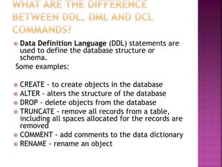
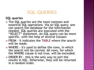
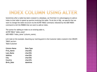
56.  Once a table is created in the database, there are many occasions where one may wish to change
the structure of the table. In general, the SQL syntax for ALTER TABLE is,
 ALTER TABLE "table_name"
[alter specification];
 [alter specification] is dependent on the type of alteration we wish to perform. We list a number
of common changes below:
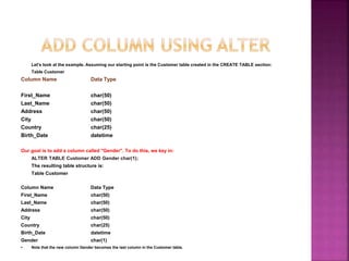
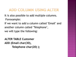
 ADD COLUMN
 MODIFY COLUMN
 RENAME COLUMN
 DROP COLUMN
 ADD INDEX
 DROP INDEX
 ADD CONTRIANT
 DROP CONSTRAINT

57. Let us take one by one and learn it how it
works:
ADD COLUMN USING ALTER
Sometimes we wish to add a column to a table.
This can be achieved in SQL. To do this, we specify
that we want to change the table structure via the
ALTER TABLE command, followed by the ADD
command to tell the RDBMS that we want to add a
column.
The SQL syntax for ALTER TABLE Add Column is,
ALTER TABLE "table_name"
ADD "column_name" "Data Type";

58. Let's look at the example. Assuming our starting point is the Customer table created in the CREATE TABLE section:
Table Customer
Column Name Data Type
First_Name char(50)
Last_Name char(50)
Address char(50)
City char(50)
Country char(25)
Birth_Date datetime
Our goal is to add a column called "Gender". To do this, we key in:
ALTER TABLE Customer ADD Gender char(1);
The resulting table structure is:
Table Customer
Column Name Data Type
First_Name char(50)
Last_Name char(50)
Address char(50)
City char(50)
Country char(25)
Birth_Date datetime
Gender char(1)
• Note that the new column Gender becomes the last column in the Customer table.

59. It is also possible to add multiple columns.
Forexample:
If we want to add a column called "Email" and
another column called "Telephone",
we will type the following:
ALTER TABLE Customer
ADD (Email char(30),
Telephone char(20) );

60. The table now becomes:
• Table Customer
Column Name Data Type
First_Name char(50)
Last_Name char(50)
Address char(50)
City char(50)
Country char(25)
Birth_Date datetime
Gender char(1)
Email char(30)
Telephone char(20)

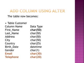
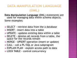
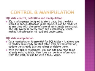
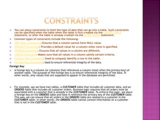
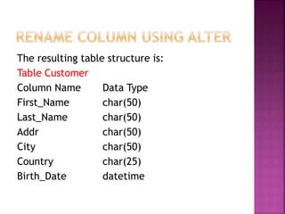
61.  Sometimes we want to change the name of a
column. To do this in SQL, we specify that we
want to change the structure of the table using
the ALTER TABLE command, followed by a
command that tells the relational database that
we want to rename the column. The exact
syntax for each database is as follows:
 In MySQL, the SQL syntax for ALTER TABLE
Rename Column is,
ALTER TABLE "table_name"
Change "column 1" "column 2" ["Data Type"];
 In Oracle, the syntax is,
ALTER TABLE "table_name"
RENAME COLUMN "column 1" TO "column 2";

62. Let's look at the example.
Assuming our starting point is the Customer table created in the CREATE
TABLE section:
Table Customer
Column Name Data Type
First_Namechar(50)
Last_Name char(50)
Address char(50)
City char(50)
Country char(25)
Birth_Date datetime
To rename "Address" to "Addr", we key in,
MySQL:
ALTER TABLE Customer CHANGE Address Addr char(50);
Oracle:
ALTER TABLE Customer RENAME COLUMN Address TO Addr;

63. The resulting table structure is:
Table Customer
Column Name Data Type
First_Name char(50)
Last_Name char(50)
Addr char(50)
City char(50)
Country char(25)
Birth_Date datetime

64. Sometimes we will wish to delete a column from an existing
table in SQL. To do this, we specify that we want to change
the table structure via the ALTER TABLE command, followed
by a specification indicating that we want to remove a
column.
The detailed syntax for each database is as follow:
In MySQL,
the syntax for ALTER TABLE Drop Column is, ALTER TABLE "table_name“
DROP "column_name";
In Oracle and SQL Server,
the syntax for ALTER TABLE Drop Column is, ALTER TABLE "table_name“
DROP COLUMN "column_name";

65. Let's look at the example. Assuming our
starting point is the Customer table created
in the CREATE TABLE section:
 Table Customer
Column Name Data Type
First_Name char(50)
Last_Name char(50)
Address char(50)
City char(50)
Country char(25)
Birth_Date datetime

66. Our goal is to drop the "Birth_Date" column. To do this, we key in:
MySQL:
ALTER TABLE Customer DROP Birth_Date;
SQL Server:
ALTER TABLE Customer DROP COLUMN Birth_Date;
Oracle:
ALTER TABLE Customer DROP COLUMN Birth_Date;
The resulting table structure is:
Table Customer
Column Name Data Type
First_Name char(50)
Last_Name char(50)
Address char(50)
City char(50)
Country char(25)

67. An index is used to speed up the
performance of queries. It does this by
reducing the number of database data
pages that have to be visited/scanned. In
SQL Server, a clustered index determines
the physical order of data in a table. There
can be only one clustered index per table
(the clustered index IS the table).

68. Sometimes after a table has been created in a database, we find that it is advantageous to add an
index to that table to speed up queries involving this table. To do this in SQL, we specify that we
want to change the table structure via the ALTER TABLE command, followed by the ADD INDEX
command to tell the RDBMS that we want to add an index.
The syntax for adding an index to an existing table is,
ALTER TABLE "table_name"
ADD INDEX "index_name" (column_name);
Let's look at the example. Assuming our starting point is the Customer table created in the CREATE
TABLE section:
Table Customer
Column Name Data Type
First_Name char(50)
Last_Name char(50)
Address char(50)
City char(50)
Country char(25)
Birth_Date datetime

69. Assume we want to add an index on the "Country“
column.
To do this, we type in the following:
 ALTER TABLE Customer ADD INDEX IDX_COUNTRY
(Country);

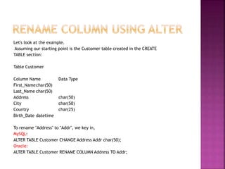
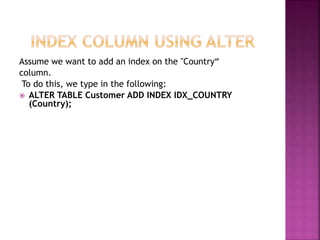
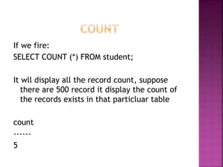
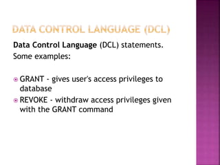
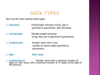
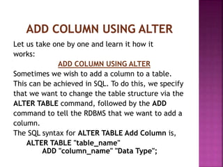
70. Select (SQL) The SQL SELECT statement returns
a result set of records from one or more tables.
A SELECT statement retrieves zero or more rows
from one or more database tables or database
views. In most applications, SELECT is the most
commonly used data manipulation language
(DML) command.
Syntax:
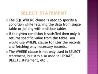
The basic syntax of SELECT statement with WHERE
clause is as follows:
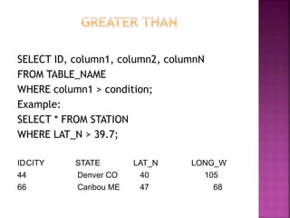
SELECT column1, column2, columnN
FROM table_name
WHERE [condition]

71.  The SQL WHERE clause is used to specify a
condition while fetching the data from single
table or joining with multiple tables.
 If the given condition is satisfied then only it
returns specific value from the table. You
would use WHERE clause to filter the records
and fetching only necessary records.
 The WHERE clause is not only used in SELECT
statement, but it is also used in UPDATE,
DELETE statement, etc.,

72. It is simplest of all & most frequently used query. Just
type
SELECT * FROM student;
The result of this query will be a display of all rows
present in the table.
ID Name Age
1 Alan 28
2 Amy 26
3 Bob 27
4 Chris 28
5 Dan 26

73. SELECT ID, column1, column2, columnN
FROM TABLE_NAME
WHERE column1 > condition;
Example:
SELECT * FROM STATION
WHERE LAT_N > 39.7;
IDCITY STATE LAT_N LONG_W
44 Denver CO 40 105
66 Caribou ME 47 68

74. If there are a huge number of rows in a table
and we do not want all the records to fill our
display screen, then SQL gives us an option to
view only selected rows.
SELECT COUNT(1) FROM student;
The output of this query will be
ID Name Age
1 Alan 28

75. If we fire:
SELECT COUNT (*) FROM student;
It wll display all the record count, suppose
there are 500 record it display the count of
the records exists in that particluar table
count
------
5