Introduction: What ispower system?
Wind
Energy
Solar
Energy
Sources of Energy
Fossil
Fuel
Nuclear
Energy
Hydro
Energy
Conventional sources
Renewable Sources
Heat generation
Steam production
Turbine
K.E.- Gen
Electrical Electrical Energy to
Kinetic Energy
Light
Heat
Chemical Energy
Utilization of Energy
Again other
form of Energy
power delivery system
5/28/2021 AKM/power system-ii/introduction 2
Electricity Generation & Utilization
3.
Big Query
• Electricityneither available naturally nor utilized in the same form
then why this intermediate form?
Possible answer:
• Transportation cost Economical
• Valid for some sources like fossil fuel (coal pit to utilization site)
• Uranium transportation cost much less than the cost required to deliver
electrical energy generated by it
Major reasons:
• Some form of energy can’t be transported
• Nature (hydro/wind)
• Potential risk (nuclear) far from public settlement
• Ease/Fast control
5/28/2021 AKM/power system-ii/introduction 3
4.
Power delivery system
•Since there may be many sources (generation of electricity) and also
several loads;
• The individual source may supply to individual or a group of loads
The primary mission is to deliver power from source (generation) to
electrical consumers at their place of consumption and in ready to use
form.
Pg(t) Pd(t)
power delivery system
Pg1(t) Pd1(t)
Pg2(t) Pd2(t)
power delivery system
power delivery system
However in actual its achieved in some different way;
5/28/2021 AKM/power system-ii/introduction 4
5.
5/28/2021 AKM/power system-ii/introduction5
However in actual; its like this
Pg1(t)
Power delivery
System
Pd1(t)
Pg2(t)
Pgn(t)
Pd2(t)
Pdm(t)
Transformers Because ;
• Its economical to generate electricity
relatively at lower voltage
• Also different generators may have
different gen. Voltage
Called Grid
6.
132 kV
The interconnectinglines need not necessarily be
at the same voltage
At the interconnection points:
only same voltage links
can be connected together
5/28/2021 AKM/power system-ii/introduction 6
It can be justified that more the power & distance
higher would be the optimum (economical) voltage
In short;
The high voltage lines are high capacity lines
But also high cost
Thus go for higher voltage only if its truly required
7.
132 kV
Towards consumer
Towardsconsumer
Towards consumer
Distribution of Energy supply
Distribution of Energy supply
Distribution of Energy supply
5/28/2021 AKM/power system-ii/introduction 7
The energy has to be delivered ultimately to consumers
8.
Why The severalsources & Loads are interconnected?
1. Exploitation of demand diversity
0
10
20
30
40
50
60
70
80
1 2 3 4 5 6 7 8 9 10 11 12 13 14 15 16 17 18 19 20 21 22 23 24
Demand
(MW)
hrs
Demand diversity
Demand1 Demand2
d1+d2 Reduced Generation capacity
Also: Reduced line capacity
5/28/2021 AKM/power system-ii/introduction 8
Pg1(t)
Pg2(t)
Pd1(t) Pd2(t)
+
Its always true that diversity seen near
the source (bulk power) is higher than
near the consumers
Pd1 & Pd2 may be at different location
9.
2. To AvoidGeneration intermittency (important with growing popularity
of Renewable these days)
Pg1(t) Pd1(t)
Pg2(t)
Pd2(t)
+
5/28/2021 AKM/power system-ii/introduction 9
• Pg1 utilized when source available (water can be stored/
fuel cost saved )
• Else Pg2 to avoid renewable intermittency
(Generation diversity)
Solar or Wind
Gen.
PROR Hydro
Or
Thermal Gen.
WU1
3. Improving reliability
Requirement:
Generatorsand transmission lines should have redundant capacity:
capable to meet contingency back up (additional cost)
5/28/2021 AKM/power system-ii/introduction 10
Pg1(t)
Pg2(t)
Pd1(t) Pd2(t)
+
better reliability if an
additional redundant line will be connected
Much better
reliability
Level of reliability depends on redundancy on generation and lines
1500 MW
demand
Dispatch
1000 MW
Dispatch
50MW
Dispatch 300 MW;
highest price
$100/MWh
Dispatch
50 MW
Dispatch
50 MW
Dispatch
50 MW
M W
N
150 MW
flow
1200 MW
flow
Reduced operational energy cost
Transmission line constraints may limit ability to use lower cost power
5/28/2021 AKM/power system-ii/introduction 12
Interconnection
Increases
Flexibility
14.
5/28/2021 AKM/power system-ii/introduction13
5. Two major Technical advantage
1. Loading effect: Terminal Voltage
V=E-Z.I
Generators in parallel
• Parallel connection reduces the overall impedance
• Loading effect is minimum (less voltage drop)
Ideally:
• if infinite number of generators connected in parallel
• Equivalent impedance is zero and no loading effect (Infinite Bus)
Terminal Voltage
V=E-ZeqI
15.
2.Frequency fluctuation
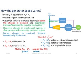
• WithChange in demand
• Instantaneously demand/generation mismatch
• Resulting mismatch in electrical output/mechanical input (Electrical change
fast but mechanical slow)
• Causes change in K.E. of the turbine/generator: change in speed (frequency)
• This is minimized by increasing the inertia (by large Fly wheel)
• Later in this course; it will be justified that;
• Equivalent inertia of an integrated system (several generators together) is
addition of the individual generation inertia
• For several no. of generators iner a tends to ∞
• Ideally no frequency fluctuation
Infinite bus:
No voltage and frequency fluctuation
5/28/2021 AKM/power system-ii/introduction 14
16.
Issues related tointerconnection
• Complexity in analysis
Pg(t) Pd(t)
Radial system
Network (Grid) system
5/28/2021 AKM/power system-ii/introduction 15
Complexity increases further
Solving the power flow in different transmission links and obtaining
the interconnection points (called Bus) voltage
Known as power flow (popularly load flow analysis)
Bus1
Bus2
Bus3
Bus4
17.
Issues related tointerconnection
• Faults aggravated and complex to analyze
Pg(t) Pd(t)
Radial system
Network (Grid) system
5/28/2021 AKM/power system-ii/introduction 16
Complexity increases further
Called Fault analysis
Bus1
Bus2
Bus3
Bus4
18.
Issues related tointerconnection (contd)
• Stability issues
Pg(t) Pd(t)
Radial system
Network (Grid) system
5/28/2021 AKM/power system-ii/introduction 17
In this course;
We deal with the issues related to interconnected system
1. Power flow solutions (popularly known as load Flow)
2. Fault analysis (Balanced/unbalanced)
3. Grid Stability (Maintaining the synchronism)
Electrical power system
Lastclass
• Importance of Electrical Energy
(energy resources to electrical
energy an its again utilized in some
form)
• Different sources (generators) are
interconnected and energy is
transported to utilization points by
power delivery system
• Power delivery system
• Transmission lines (system): Bulk
power Near the source (Higher
voltage)
• Distribution lines (system): Near
consumption (relatively Lower voltage)
Change in demand (real and/or
reactive power) Generators need
to respond
How?
Characteristic difference in P &Q
5/28/2021
AKM/power system-ii/P&Q balance 2
21.
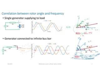
Real Power Control
•Real power related to energy
• Some form of energy input → Electrical
energy as an output
• Electrical load not always remains constant
• With variation of electrical demand the
input energy should also vary
• Governor controls the valve opening; it
sense the change in demand and
accordingly increase/decrease the input to
the turbine
Governor
Generator
Turbine
Input
Steam/water
Output
Electrical Energy
Load
Control Valve
• Input to the governor is generator frequency
(speed)
• Increase in frequency → demand decrement
→ decrease in input
• Decrease in frequency → demand increment
→ increase in input
5/28/2021 AKM/power system-ii/P&Q balance 3
22.
Governor Operation Roleof Fly wheel & Governor
Governor Fly wheel
Controls mean speed Limit cyclic
fluctuations in speed
Mathematically
controls dω
Controls dω/dt
Adjust demand/supply
energy
No influence on
supply/demand
How the Governor controls the input to
match the demand and supply exactly?
5/28/2021 AKM/power system-ii/P&Q balance 4
23.
Frequency droop characteristic
•Governor poses a Power-frequency droop characteristic
• The slope is measured in percent of frequency change
• A typical slope is 5%, means that if frequency error is 5%
the full output of the generator would be used to
counteract the frequency error.
• The drop in frequency is the indicative of change in real
power demand
Frequency
Power
R=
∆
∆
Example:
Governor gives the control signal to the valve to decrease the turbine output of 2 MW
A 500 MVA, 50 Hz, generating unit has a regulation constant R of 0.05 p.u. on
its own rating. If the frequency of the system increases by 0.01 Hz in the
steady state, what is the decrease in the turbine output?
Solution:
In p.u. ∆f = 0.01/50 = 0.0002 p.u.
∆pm = -1/R(∆f) = - 0.004 p.u. = - 2 MW.
5/28/2021 AKM/power system-ii/P&Q balance 5
24.
Load sharing amongthe generators
• Lets consider a system with three generators & loads
• Suppose system operates at frequency of f1 with demand and
supply balance Pg1+Pg2 +Pg3 =Pd2+ Pd3+Pd4 + Ploss
• If the system demand increased by ΔPd
• What will be new operating frequency f2 and how the generators
share incremental demand ?
f2
Pg1’ Pg2’ Pg3’
Pg1 Pg2 Pg3
f1
R2
R1 R3
𝑅1 =
𝑓1 − 𝑓2
𝑃𝑔1 − 𝑃𝑔1′
= −
∆𝑓
∆𝑃𝑔1
𝑅2 =
𝑓1 − 𝑓2
𝑃𝑔2 − 𝑃𝑔2′
= −
∆𝑓
∆𝑃𝑔2
𝑅3 =
𝑓1 − 𝑓2
𝑃𝑔3 − 𝑃𝑔3′
= −
∆𝑓
∆𝑃𝑔3
5/28/2021 AKM/power system-ii/P&Q balance 6
25.
For n generatorsystem
Important:
• Not all the generators may participate to share the
incremental demand. The reasons;
• Economical generator operation
• System constraints
• Considering Load frequency control together with
economical generator operations known as AGC
control
• In reality, only a few generators participate for load
frequency balancing (Centrally controlled at Load
Dispatch Center )
∆𝑓 =
1
1
𝑅1 + 1
𝑅2 + ⋯ + 1
𝑅𝑛
∆𝑃𝑑
∆𝑃𝑔𝑖 =
1
𝑅𝑖
∆𝑓
And Generator with lesser R
share more demand
5/28/2021 AKM/power system-ii/P&Q balance 7
26.
Assignment:
1. An interconnected50 Hz power system consists of three generating
units. The regulation constant of each unit is R= 0.05 per unit on its
own rating. Each unit is initially operating at one half of its rating, when
the system load suddenly increases by 200MW. Determine the steady
state frequency deviation of the area, and the increase in turbine
power output. If the generator ratings are
• A. 500 each
• B. 500 MW, 750 MW and 1000 MW respectively
2. Repeat the Above problem if the regulation constants of the generators
are 0.04 p.u.,0.05 p.u. and 0.06 p.u. on its own rating respectively
5/28/2021 AKM/power system-ii/P&Q balance 8
27.
Arbind K. Mishra
IOE,Pulchowk Campus
5/28/2021 AKM/power system-ii/L3/Reactive power balance
1
28.
Last Class
• Realpower demand and supply balance is associated
with Frequency
• increase in electrical power demand frequency drops
• decrease in demand frequency increases
• From power quality point of view high frequency
fluctuation is not desirable
• However Governor use this (information) variation to
Adjust demand/supply energy to the generator
• It does so utilizing frequency droop characteristic
• The slope of the frequency droop is measured in
percent of frequency change
• The drop/rise in frequency is the indicative of
amount of real power demand change
• Governor control the valve opening (at the input) to
increase/decrease the required input energy with
change in electrical demand
5/28/2021 AKM/power system-ii/L3/Reactive power balance 2
29.
For multiple generatorsystem
However:
• Not all the generators may participate to share the incremental demand.
The reasons;
• Economical generator operation
• System constraints
• In reality, only a few generators participate for load frequency balancing
(Centrally controlled at Load Dispatch Center )
∆𝑓 =
1
1
𝑅1 + 1
𝑅2 + ⋯ + 1
𝑅𝑛
∆𝑃𝑑
∆𝑃𝑔𝑖 =
1
𝑅𝑖
∆𝑓
And
Generator with lesser R share more demand
5/28/2021 AKM/power system-ii/L3/Reactive power balance 3
30.
Assignment:
1. An interconnected50 Hz power system consists of three generating
units. The regulation constant of each unit is R= 0.05 per unit on its
own rating. Each unit is initially operating at one half of its rating, when
the system load suddenly increases by 200MW. Determine the steady
state frequency deviation of the area, and the increase in turbine
power output. If the generator ratings are
• A. 500 each
• B. 500 MW, 750 MW and 1000 MW respectively
2. Repeat the Above problem if the regulation constants of the generators
are 0.04 p.u.,0.05 p.u. and 0.06 p.u. on its own rating respectively
5/28/2021 AKM/power system-ii/L3/Reactive power balance 4
31.
Solution: Q1.A
• 50Hz power system consists of three generating units 500 MVA each
• The regulation constant of each unit is R= 0.05 per unit on its own rating
• From initial operating load increases by 200MW
• Determine
• steady state frequency deviation
• the increase in turbine power output
5/28/2021 AKM/power system-ii/L3/Reactive power balance 5
500 MW 500 MW 500 MW
2.5 Hz
32.
Solution: Q1.B
• 50Hz power system consists of three generating units 500 MVA , 750 MVA & 1000 MVA
• The regulation constant of each unit is R= 0.05 per unit on its own rating
• From initial operating load increases by 200MW
• Determine
• steady state frequency deviation
• the increase in turbine power output
5/28/2021 AKM/power system-ii/L3/Reactive power balance 6
33.
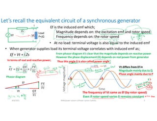
Loading effect onSynchronous generator
Ef
Zs
Load
P+jQ
Vt
I
Ef = Vt + I.Zs Vt.I*=P+jQ
𝐸𝑓 = 𝑉𝑡 +
𝑄𝑋
𝑉𝑡
+ 𝐽
𝑃𝑋
𝑉𝑡
𝐸𝑓 = 𝑉𝑡 +
𝑄𝑋
𝑉𝑡
+
𝑃𝑋
𝑉𝑡
Vt 𝑄𝑋
𝑉𝑡
𝑃𝑋
𝑉𝑡
Ef
δ
5/28/2021 AKM/power system-ii/L3/Reactive power balance 7
34.
Terminal Voltage Controlof a Synchronous generator
Ef
Zs
Load
P+jQ
Vt
I
𝐸𝑓 = 𝑉𝑡 +
𝑄𝑋
𝑉𝑡
+ 𝐽
𝑃𝑋
𝑉𝑡
𝐸𝑓 ≈ 𝑉𝑡 +
𝑄𝑋
𝑉𝑡
Vt 𝑄𝑋
𝑉𝑡
𝑃𝑋
𝑉𝑡
Ef
δ
5/28/2021 AKM/power system-ii/L3/Reactive power balance 8
Vt≈ 𝐸𝑓 −
• Real power variation has almost no effect on terminal
voltage magnitude
• Terminal voltage (magnitude) is heavily effected by
variation in reactive power
• Options:
• Keep the reactive power generation always constant
• Allow the reactive power generation to vary but terminal voltage to
vary
• Allow the reactive power generation to vary and also control the
terminal voltage (Called voltage controlled Bus)
• How ?
35.
Voltage Controlled Bus
•Vary the Ef (by varying the excitation flux)
• Reactive power demand could be lagging/leading
• More and more Lagging Q means higher & higher field current (must have some limit)
poses maximum Qlmt in lagging mode
• More and more Q in leading mode (under excitation) but δ goes on increasing not
desirable (will be discussed later)
• Hence a generator Bus can operate as a voltage controlled bus but within a limit of
reactive power supply only.
5/28/2021 AKM/power system-ii/L3/Reactive power balance 9
Ef
Zs
Load
P+jQ
Vt
I
Vt≈ 𝐸𝑓 −
Load Flow analysis
•In a power system, different sources
(generators) and Loads are interconnected
through transmission lines
• In the System its often essential to know;
• Power flow through different components
• Voltage at various buses
• Component wise and overall system losses
(if undesirable, Prior correction(s) can be taken)
• This analysis is known as load flow (power
flow) analysis
• A load flow analysis displays the mathematical
description of an electrical network, as well as
calculations that arrive at results
5/31/2021 AKM/power system-ii/L4/Load Flow Analysis 2
38.
• A powerflow (Load flow) study refers to
the steady state analysis of a power network. It
will determine how the system will operate
depending on the given loading.
• For operations, Load flow studies are done to
make sure that every generator reaches its
optimal operating capacity, not only at normal
operations but also maintenance can be
conducted safely, and power supply can meet
the demand satisfactorily
• Load flow analysis are utilized in planning and
design studies to establish whether a specific
element in the infrastructure is at risk for
overloading or not.
5/31/2021 AKM/power system-ii/L4/Load Flow Analysis 3
39.
• In essenceload flow analysis are done to evaluate;
• Power flow through different components
• Bus voltage
• Components and system losses
• However the first task in the load flow is to know
the bus voltage magnitude and phase angle at all
the buses (Why?)
Lets consider a branch of the network
Line
parameters
Vs, δs Vr, δr
Already know the expressions for
Ps, Qs, Pr And Qr
The difference between Ps & Pr real power loss And
The difference between Qs & Qr reactive power loss
Negative power flow means power flow direction is opposite of that assumed
Ps Qs Pr Qr
5/31/2021 AKM/power system-ii/L4/Load Flow Analysis 4
40.
How to evaluatevoltage at each bus?
• Power system buses besides
interconnecting lines, are also connected
with;
• Source (generation)
• Loads
Bus2
Bus1
Bus3
Bus4
Generators inject the power (real & reactive) to the system
Load draws power from the system
I1
I2
I3
I4
That is each
bus can be
thought to
inject an
equivalent
current
5/31/2021 AKM/power system-ii/L4/Load Flow Analysis 5
41.
• Different linescan be modeled as;
• Short line model
• Medium line model
• Long line model
Equivalent π model
5/31/2021 AKM/power system-ii/L4/Load Flow Analysis 6
42.
• Replace therespective line by ;
• Short line : short line model
• Medium line: nominal π-model
• Long line: equivalent π-model
Applying KCL at each node;
Z23
y20
y40
y10
y30
5/31/2021 AKM/power system-ii/L4/Load Flow Analysis 7
43.
Some peculiarities ofabove matrix
• Square matrix of 4 x 4 (For a N bus system N x N)
• Symmetric matrix
• Elements of the matrix are only the physical
parameters (Don’t depends on loading condition)
• Diagonal elements Yii : shunt admittance at the node +
sum of the branches series admittance connected to
the node
• Off diagonal elements Yij : negative of branch series
admittance connected between ith & jth node
In Short;
In short, The Matrix follows a systematic formulation
and no need to derive each time
y23
y20
y40
y10
y30
5/31/2021 AKM/power system-ii/L4/Load Flow Analysis 8
[ IBUS ] = [ Matrix ] [VBUS]
Popularly know as:
Bus admittance matrix
YBUS Matrix
Last Class
• LoadFlow analysis is an important
mathematical tool for analyzing the system
performance;
• satisfactory operational decision
• Optimal planning & design
• System performance analysis includes;
• Power flow through different components of
the network
• Voltage at various buses
• Component wise and overall system losses
6/3/2021 AKM/power system-ii/L5/Load Flow Equations 2
• For load flow, the first step is to know the bus voltages at each buses
• So if bus voltage at a particular bus is known ok, otherwise first
compute bus voltages at those buses before other computations;
46.
Characteristics of theBus admittance (YBUS )matrix;
• Square matrix, of size n x n (For a n bus system)
• Symmetric matrix
• Elements of the matrix are only the physical parameters (r.l,c)
(Don’t depends on loading condition)
6/3/2021 AKM/power system-ii/L5/Load Flow Equations 3
[ IBUS ] = [ YBUS ] [VBUS]
• Correlation between Bus injected current vector and bus voltage vector
Elements of the Ybus Matrix are defined as;
• Diagonal elements Yii : shunt admittance at the node + sum of the branches series admittance
connected to the node
• Off-diagonal elements Yij : negative of branch series admittance connected between ith & jth
node
(That is, for a given network it needs to be computed only once)
47.
Example Compute theYBUS Matrix For;
E1. A Two Bus system J20 Ω
1 2
E2. A Two Bus system line parameter in p.u.
J0.2
1 2
J0.05 J0.05
6/3/2021 AKM/power system-ii/L5/Load Flow Equations 4
1 2
J0.05 J0.05
1 2
48.
E3. A 3Bus System
J0.2
1 2
3
J0.1 J0.1
J0.1 J0.1
Convert
impedances to
admittance
6/3/2021 AKM/power system-ii/L5/Load Flow Equations 5
1 2
3
J0.1 J0.1
49.
Assignment: Compute theBus Admitance matrix for;
Line Z = j0.07
Line Z = j0.05 Line Z = j0.1
One Two
200 MW
100 MVR
Three 1.000 pu
200 MW
100 MVR
34.3 14.3 20
14.3 24.3 10
20 10 30
bus j
Y
Question:1
Question:2
1 4
2
3
5
From-to R (p.u) X(p.u) B/2
1-2 0.1 0.4 -
1-4 0.15 0.6 -
1-5 0.05 0.2 -
2-3 0.05 0.2 -
2-4 0.10 0.4 -
3-5 0.05 0.2 -
6/3/2021 AKM/power system-ii/L5/Load Flow Equations 6
0
0
0 0
0
0
0
0
Meaning of element 0 ?
Application of YBUSMatrix
• For any general system;
• So Bus Voltages can be calculated as;
• ZBUS is called Bus Impedance matrix
• However ZBUS Matrix is rarely computed by inverse of YBUS Matrix
• There are methods to compute ZBUS Matrix directly
• But by whatever methods YBUS or ZBUS Matrixes would be computed, the
above expression can be used to compute Bus voltages only if bus injected
currents are known explicietly
[ IBUS ] = [ YBUS ] [VBUS]
[ VBUS ] = [ YBUS ]-1 [IBUS]
[ VBUS ] = [ ZBUS ] [IBUS]
(because for a practical system YBUS Matrix is a sparse matrix & often its not possible to
compute its inverse)
6/3/2021 AKM/power system-ii/L5/Load Flow Equations 9
53.
• The businjected complex power and currents
are correlated by;
Si = Vi Ii
*
• Also; Bus voltage and injected currents are
correlated as;
s1
S2
S3
S4
6/3/2021 AKM/power system-ii/L5/Load Flow Equations 10
∗
Known as Fundamental
Load Flow equations;
𝐼
𝐼
…
𝐼
𝑉
𝑉
…
𝑉
54.
∗
Altogether 2n Numberof equations
• At each buses 4 Variables (4n Variables)
Bus2
Bus1
Bus3
Bus4
Based on
• Quantities (variables) known
• Quantities (variables) need to be computed
Power system buses are classified
P1+JQ1
P2+JQ2
P4+JQ4
P3+JQ4
V1 , δ1
V2 , δ2
V4 , δ4
V3 , δ3
• 2n Variables must be known
6/3/2021 AKM/power system-ii/L5/Load Flow Equations 11
55.
Arbind K. Mishra
IOE,Pulchowk Campus
6/7/2021 AKM/power system-ii/L6/solution of Load Flow Equations
1
56.
• Altogether 2nNumber of equations
• At each buses 4 Variables (total 4n Variables)
• 2n variables must be specified to solve these
equations
Bus2
Bus1
Bus3
Bus4
Based on
• Quantities (variables) known
• Quantities (variables) need to be computed
Power system buses are classified
P1+JQ1
P2+JQ2
P4+JQ4
P3+JQ4
V1 , δ1
V2 , δ2
V4 , δ4
V3 , δ3
6/7/2021 AKM/power system-ii/L6/solution of Load Flow Equations 2
Fundamental Load Flow
equations;
Last Class:
𝑃 − 𝑗𝑄
𝑉∗ = 𝑌 𝑉
57.
Bus Classification
Bus Type
Known
(Specified)
Variables
Variables
tobe
computed
Load Bus
(PQ Bus)
P & Q V & δ
Generator Bus
(Voltage Controlled Bus)
(PV Bus)
P & V Q & δ
Reference Bus
(Slack Bus)
(Swing Bus)
V & δ P & Q
Bus2
Bus1
Bus3
Bus4
Note: Generators at generator buses are also specified with Qgi limit
6/7/2021 AKM/power system-ii/L6/solution of Load Flow Equations 3
58.
Solution techniques:
• Needssome iterative techniques to solve
• The iterative methods are characterized by the various performance features
• One of the iterative techniques used for load Flow analysis is Gauss-Siedel
Method
Load flow equations are Non-linear
equations
• Is an iterative algorithm for solving non linear algebraic equations.
• An initial solution vector is assumed (chosen from practical/past experiences)
• At every subsequent iteration, the solution is updated till convergence is
reached.
Gauss-Siedel (G-S) Method
𝑃 − 𝑗𝑄
𝑉∗ = 𝑌 𝑉
6/7/2021 AKM/power system-ii/L6/solution of Load Flow Equations 4
59.
Gauss-Siedel (G-S) Method
•Important: iterative techniques are needed only
to know Bus Voltages
• Re arrange the load flow equations in terms of ith
bus Voltage;
𝑃 − 𝑗𝑄
𝑉∗ = 𝑌 𝑉
6/7/2021 AKM/power system-ii/L6/solution of Load Flow Equations 5
In iterative procedure equation
can be re-written as;
• for bus-i, updated values are already available for buses up to (i-1) in the current iteration.
• For buses (i+1)…..n, values from previous iterations, are used.
60.
Algorithm for GSmethod
Suppose all the buses (except slack bus) are load buses
1. Read physical parameters & specified Bus variables
2. Formulate the bus admittance matrix YBUS
3. Start iteration count k=0; Assume initial voltages for all
buses; [In practical power systems, the magnitude of the bus
voltages is close to 1.0 p.u. Hence, the voltages at all (n-1) buses
(except slack bus) may be assumed to be 1.0+j0]
4. increase iteration count k=k+1
5. For i=2 to n; Update the voltages given by;
Bus2
Bus1
Bus3
Bus4
6. Check convergence criterion If not go back to step 4
7. Compute slack bus power
6/7/2021 AKM/power system-ii/L6/solution of Load Flow Equations 6
With assumption bus 1 is slack bus
61.
Example
1. System parameter& specified variables
Z=j0.5 , & S2 = 0-(0.5+j0)=-0.5-j0
2. Formulate YBUS matrix
3. Set iteration k=0 & assume unknown voltage
4. For i=2 to n; Update the voltages given by;
For this example it is;
After 4th iteration;
After 5th iteration;
6/7/2021 AKM/power system-ii/L6/solution of Load Flow Equations 7
0.5+j0
62.
Example 2
6/7/2021 AKM/powersystem-ii/L6/solution of Load Flow Equations 8
Line Z = j0.07
Line Z = j0.05 Line Z = j0.1
One Two
200 MW
100 MVR
Three 1.000 pu
200 MW
100 MVR
All the impedance are at
Rated voltage and 1000 MVA base
1. System parameter & specified variables
: ,
S2 = -0.2 - j0.1 & S3 = -0.2 - j0.1
3. Set iteration k=0 & assume unknown voltage
4. For i=2 to n; Update the voltages given by;
34.3 14.3 20
14.3 24.3 10
20 10 30
bus j
Y
3
2. Formulate YBUS matrix
63.
Consideration of Generatorbus in G-S method
• At generator Buses
• Known Quantities (variables) P & V Magnitude
• To be known Q and δ
• First Find Qi :
• Compute Qgi = Qi +Qdi
• Check Qgi limit:
6/7/2021 AKM/power system-ii/L6/solution of Load Flow Equations 9
𝑃 − 𝑗𝑄
𝑉∗ = 𝑌 𝑉
If Qgi ˂ Qgi min. lmt Qgi = Qgi min. lmt Qi = Qgi min. lmt - Qdi
&
If Qgi ˃ Qgi max. lmt Qgi = Qgi max. lmt Qi = Qgi max. lmt - Qdi
&
In both of these condition; Qi is now fixed
• Else If Qgi calculated is within limit, Qi will be as calculated and V magnitude will be as
specified and δ need to be calculated
That is; if Qgi is either less than min limiting value or greater than maximum limiting value the
voltage cannot be maintained at the specified value due to lack of reactive power support.
& for this iteration this bus is virtually treated as load bus;
64.
Complete Algorithm forGS method
1. Read physical parameters & specified Bus variables
2. Formulate the bus admittance matrix YBUS
3. Start iteration count k=0; Assume initial voltages for all
load buses and bus voltage angle at generator buses
4. Increase iteration count k=k+1
5. Start bus count i=1
6. Check is it slack bus ?; yes: i=i+1
7. Check is it generator bus? No: go to step 8
Compute bus reactive power as;
6/7/2021 AKM/power system-ii/L6/solution of Load Flow Equations 10
Check Qgi within limit ? if yes Qi as calculated
if not set Qi = Qgi lmt - Qdi and go to step 8 (treat load Bus)
Bus2
Bus1
Bus3
Bus4
65.
8. Update thebus voltages as;
10. Check convergence criterion If not k = k+1 & go back to step 4
11. Compute slack bus power Suffix 1: with assumption bus 1 is
slack bus
6/7/2021 AKM/power system-ii/L6/solution of Load Flow Equations 11
Compute bus voltage as;
[Since Voltage magnitude is specified at PV bus]
Go to step 9
9. Increase bus count i=i+1; if I ˂= n go to step 6
LFA: What wehave discussed so for?
2. Load Flow equations
1. Given a Network; YBUS Matrix
can be computed
Matrix elements depends only
on the physical parameters
For a given network don’t
change with loading
𝑃 − 𝑗𝑄
𝑉∗ = 𝑌 𝑉
3. The L.F. equations may be re-arranged
depending on quantities to be computed;
Correlates Bus Voltage &
injected real and reactive
power
…(1)
Pi = Re …(2)
Qi = -Im …(3)
START
Read Specified quantities, system parameter & Compute YBUS Matrix
Set iteration count, k=0; Assume bus voltages
Increase iteration count, k=k+1
is
is slack bus ?
Start bus count, i=1
is
is Gen. bus ?
No
Calculate Qi (Eq 3)
Calculate Qgi
is
Qgi min<Qgi<Qgi max
Calculate Vi (Eq 1)
Yes
Increase bus count i=i+1
is
is i ≤ n ?
Qi =Qgi lmt + Qdi
Yes
No
Vi = Visp⟨δ𝑖
is
is
Calculate slack Bus power Eq 2 & 3 & stop
Yes
Yes
Yes No
At Load Bus Eq 1
At Gen Bus Eq 3 & Eq 1
At slack Bus Eq 2 & Eq3
G-S Method
Eq.1 need to solve at n-1 buses
requires iterative techniques No
No
Calculate Vi (Eq 1)
AKM/power system-ii/L7/LFA solution contd
68.
Acceleration factor inG-S method
• It is found that in GS method, the number of iterations increase with increase in the size
(number of Buses) of the system.
• The number of iterations may be reduced if the correction in voltage at each bus is
accelerated, by multiplying with a constant α (called the acceleration factor)
• The idea is; if the difference in successive iterations Quantities are large, means more
correction needed.
• If voltage at ith Bus in current iteration is and in the previous iteration hen;
𝒊
𝒌 𝟏
𝒊
𝒌
𝒊
𝒌 𝟏
- 𝒊
𝒌
)
• If value of means ?
• If value of means ?
• If value of means ?
• If too high, successive iteration values oscillates; if too low, sluggish
• Value is generally chosen between 1.2 to 1.6
No acceleration
Value closer to previous iteration
Current iteration value is extrapolated
6/9/2021 AKM/power system-ii/L7/LFA solution contd 3
69.
Limitation of G-Smethods
• GS method is an efficient method for small system
• The method is easy to be familiar with
• For a large system, the number of iterations (computation time)
becomes impractically large and convergence also depends on factors
like;
• selection of slack bus
• initial guess of solution
• Acceleration factor
• Therefore the application of G-S Method is limited only for a small
system (e.g. for a learner)
• For large (practical) system, the iterative methods called Newton-
Raphson method is more popular;
6/9/2021 AKM/power system-ii/L7/LFA solution contd 4
70.
Newton –Raphson methodfor Load Flow Analysis
6/9/2021 AKM/power system-ii/L7/LFA solution contd 5
• Suppose we have to solve a nonlinear algebraic equations y=f(x) and we know the
solution is near the point x =x0;
• We can write; y = f (x0 + Δx)
• Using Taylor’s series expansion;
• Neglecting higher order terms;
• With multiple variables;
𝑥
Δx
𝑥
x1 𝑥
x2+………….+ 𝑥
xn
=
[ Jacobean Matrix]
6/14/2021 AKM/power system-ii/L8/N-R,LF solution 2
• For set of nonlinear expressions with multiple variables;
Error vector Correction vector
Newton –Raphson iterative method
In short; Δx=J-1Δf x1=x0+ Δx0
Y1= f1 (x1, x2, x3,…. xn)
Y2= f1 (x1, x2, x3,…. xn)
Yn= f1 (x1, x2, x3,…. xn)
For example
5 = x1 + 2 x1x2
2 = x2 + x1 x3
1= x1
2 + x3
2
If 𝟏
𝟎
𝟐
𝟎
𝟑
𝟎
𝒏
𝟎 be the initial assumptions for the variables, and the corrections in
respective variables are Δx1 , Δx2 ,…… Δxn then;
Note: Possible, if J is a square matrix;
means;
number of equations must be
equal to number of variables
In general, xk+1=xk+ Δxk
76.
N-R iterative methodsfor load flow Equations
• Variable x: unknown bus voltage magnitude and phase angles
• Phase angles: at all buses( except slack bus)
• Voltage magnitude: at load buses
Pi = Re …(2)
Qi = -Im …(3)
6/14/2021 AKM/power system-ii/L8/N-R,LF solution 3
• Function f: bus injected real and reactive power expressions
(but only at those buses where real and/or reactive powers specified)
specified at all buses (except slack bus)
specified at all load buses
That is for a N-Bus system with NG number of generator buses
Number of unknown variables
Phase angle, δ
Voltage magnitude, V
Total
Number of Equations
Real Power, P
Reactive, Q
Total
Should be like;
5 = x1 + 2 x1x2
2 = x2 + x1 x3
1= x1
2 + x3
2
77.
Suppose;
• Bus 1is numbered as slack bus
• Bus 2 to (NG + 1) are numbered as Generator Buses
• Load buses are numbered from (NG + 2) to N
6/14/2021 AKM/power system-ii/L8/N-R,LF solution 4
That is for a N-Bus system with NG number of generator buses
Functions: f (bus injected real and
reactive power) vector will look like;
Network in the diagram;
5 Bus system with
2 generator buses
Variables: x (bus voltage phase angles
and magnitude) vector will look like;
Thus for N-Rmethod of load Flow analysis
6/14/2021 AKM/power system-ii/L8/N-R,LF solution 6
Δδi = correction in ith bus phase angle from estimate
ΔVi = correction in ith bus voltage magnitude from estimate
Sub Matrix of size
(N-1) x (N-1)
Sub Matrix of size
(N-1) x (N-NG - 1)
Sub Matrix of size
(N-NG - 1) x (N-1)
Sub Matrix of size
(N-NG - 1) x (N-NG - 1)
In above only challenging task is to compute the Jacobean Matrix
80.
The Jacobean Matrixelements are derivatives of Bus injected
real and reactive power w.r.t δ and V
• Lets First recall the expressions for Bus injected real and reactive
powers;
6/14/2021 AKM/power system-ii/L8/N-R,LF solution 7
Pi = Re …(2)
Qi = -Im …(3)
&
𝒊= 𝒊 𝒋 𝒊𝒋 𝒋 𝒊
𝒏
𝒋 𝟏 + 𝒊𝒋
𝒊=- 𝒊 𝒋 𝒊𝒋 𝒋 𝒊
𝒏
𝒋 𝟏 + 𝒊𝒋
𝒊= 𝒊 𝒋 𝒊𝒋 𝒊 𝒋
𝒏
𝒋 𝟏 𝒊𝒋
𝒊= 𝒊 𝒋 𝒊𝒋 𝒊 𝒋
𝒏
𝒋 𝟏 𝒊𝒋
81.
Example: For theNetwork in the diagram obtain the Jacobean Matrix
6/14/2021 AKM/power system-ii/L8/N-R,LF solution 8
𝒊= 𝒊 𝒋 𝒊𝒋 𝒊 𝒋
𝒏
𝒋 𝟏 𝒊𝒋
𝒊= 𝒊 𝒋 𝒊𝒋 𝒊 𝒋
𝒏
𝒋 𝟏 𝒊𝒋
1
2
3
82.
N-R LFA Algorithm
6/14/2021AKM/power system-ii/L8/N-R,LF solution 9
1. Read physical parameters & specified Bus variables
2. Formulate the bus admittance matrix YBUS
3. Start iteration count k=0; Assume initial voltages (Magnitude and phase angle at
Load buses and magnitude at generator buses)
4. increase iteration count k=k+1
5. Compute;
• Pcal at all buses (except Slack Bus)
• Qcal at load buses
• Error vector
6. Compute Jacobean Matrix
7. Compute the correction Vector as;
8. Compute updated value of δ and V
(k+1)= (k)+Δδi(k)
(k+1)= (k)+ΔVi(k)
Δδ
Δ𝑉
=
𝐽1 𝐽1
𝐽1 𝐽1
Δ𝑃
Δ𝑄
Δ𝑃
Δ𝑄
𝑷𝒊=∑ 𝑽𝒊 𝑽𝒋 𝒀𝒊𝒋 𝐜𝐨𝐬(𝜹𝒊 − 𝜹𝒋
𝒏
𝒋 𝟏 − 𝜽𝒊𝒋)
𝑸𝒊=∑ 𝑽𝒊 𝑽𝒋 𝒀𝒊𝒋 𝐬𝐢𝐧(𝜹𝒊 − 𝜹𝒋
𝒏
𝒋 𝟏 − 𝜽𝒊𝒋)
83.
9. Check convergencecriterion as;
error vector
If not satisfied go back in step 4 (next iteration)
10. Compute slack bus real and reactive power and Stop
6/14/2021 AKM/power system-ii/L8/N-R,LF solution 10
8. Compute Qi at generator buses
Compute Qgi = Qi +Qdi
Check Qgi limit:
If Qgi ˂ Qgi min. lmt Qgi = Qgi min. lmt Qi = Qgi min. lmt - Qdi
If Qgi ˃ Qgi max. lmt Qgi = Qgi max. lmt Qi = Qgi max. lmt - Qdi
In next iteration treat this bus as Load bus
In next iteration treat this bus as Load bus
Δ𝑃
Δ𝑄 <ε
𝒊= 𝒊 𝒋 𝒊𝒋 𝒊 𝒋
𝒏
𝒋 𝟏 𝒊𝒋
𝒊= 𝒊 𝒋 𝒊𝒋 𝒊 𝒋
𝒏
𝒋 𝟏 𝒊𝒋
𝒊= 𝒊 𝒋 𝒊𝒋 𝒊 𝒋
𝒏
𝒋 𝟏 𝒊𝒋
Last Class: N-Rload Flow analysis Formulation
6/16/2021 AKM/power system-ii/L9/N-R,DLF,FDLF& DCLF solutions 2
Δδi = correction in ith bus phase angle from estimate
At all buses except slack bus
ΔVi = correction in ith bus voltage magnitude from estimate
At all Load buses
At all buses except slack bus
At all load buses
Error Vector
Correction
Vector
Jacobean Matrix
Jacobean Matrix:
Numerical value of:
Partial derivative of P & Q w.r..t |V|
& δ at estimated Voltages
𝐽 =
𝜕𝑃
𝜕δ
P (where specified) w.r.t δ (unknown)
(N-1) x (N-1)
𝐽 =
𝜕𝑃
𝜕𝑉
P (where specified) w.r.t V (unknown)
(N-1) x (N-NG - 1)
𝐽 =
𝜕𝑄
𝜕δ
Q (where specified) w.r.t δ (unknown)
(N-NG - 1) x (N-1)
𝐽 =
𝜕𝑄
𝜕𝑉
Q (where specified) w.r.t V (unknown)
(N-NG - 1) x (N-NG - 1)
1
2
3
Slack Bus
Generator Bus
Load Bus
87.
N-R LFA Algorithm
6/16/2021AKM/power system-ii/L9/N-R,DLF,FDLF& DCLF solutions 3
1. Read physical parameters & specified Bus variables
2. Formulate the bus admittance matrix YBUS
3. Start iteration count k=0; Assume initial voltages (phase angle at all buses except
slack bus & Voltage magnitude at Load buses)
4. increase iteration count k=k+1
5. Compute;
• Pcal at all buses (except Slack Bus)
• Qcal at load buses
• Error vector
6. Compute Jacobean Matrix
7. Compute the correction Vector as;
8. Compute updated value of δ and V
(k+1)= (k)+Δδi(k)
(k+1)= (k)+ΔVi(k)
Δδ
Δ𝑉
=
𝐽1 𝐽2
𝐽3 𝐽4
Δ𝑃
Δ𝑄
Δ𝑃
Δ𝑄
𝑷𝒊=∑ 𝑽𝒊 𝑽𝒋 𝒀𝒊𝒋 𝐜𝐨𝐬(𝜹𝒊 − 𝜹𝒋
𝒏
𝒋 𝟏 − 𝜽𝒊𝒋)
𝑸𝒊=∑ 𝑽𝒊 𝑽𝒋 𝒀𝒊𝒋 𝐬𝐢𝐧(𝜹𝒊 − 𝜹𝒋
𝒏
𝒋 𝟏 − 𝜽𝒊𝒋)
𝐽1 𝐽2
𝐽3 𝐽4
88.
9. Check convergencecriterion as;
error vector
If not satisfied go back in step 4 (next iteration)
10. Compute slack bus real and reactive power and Stop
6/16/2021 AKM/power system-ii/L9/N-R,DLF,FDLF& DCLF solutions 4
8. Compute Qi at generator buses
Compute Qgi = Qi +Qdi
Check Qgi limit:
If Qgi ˂ Qgi min. lmt Qgi = Qgi min. lmt Qi = Qgi min. lmt - Qdi
If Qgi ˃ Qgi max. lmt Qgi = Qgi max. lmt Qi = Qgi max. lmt - Qdi
In next iteration treat this bus as Load bus
In next iteration treat this bus as Load bus
Δ𝑃
Δ𝑄 <ε
𝒊= 𝒊 𝒋 𝒊𝒋 𝒊 𝒋
𝒏
𝒋 𝟏 𝒊𝒋
𝒊= 𝒊 𝒋 𝒊𝒋 𝒊 𝒋
𝒏
𝒋 𝟏 𝒊𝒋
𝒊= 𝒊 𝒋 𝒊𝒋 𝒊 𝒋
𝒏
𝒋 𝟏 𝒊𝒋
89.
Comparison of N-Rmethod with G-S method
• Storage requirement in N-R Method Higher w.r.t. G-S Method
• Unlike G-S method, number of iterations are almost independent of the bus
number
• However per iteration computation time higher
• So often measures are taken to reduce computational burden & storage for
Jacobean matrix
• Lets recall the LFA Formulation;
6/16/2021 AKM/power system-ii/L9/N-R,DLF,FDLF& DCLF solutions 5
(mainly due to computation of Jacobean matrix)
𝜕𝑃
𝜕δ
𝜕𝑃
𝜕𝑉
𝜕𝑄
𝜕δ
𝜕𝑄
𝜕𝑉
Sensitivity of P w.r.t. δ
Sensitivity of P w.r.t. V
Sensitivity of Q w.r.t. δ
Sensitivity of Q w.r.t. V
(mainly due to Jacobean matrix storage)
90.
In one ofthe previous Class;
Loss less Model for a synchronous Generator
6/16/2021 AKM/power system-ii/L9/N-R,DLF,FDLF& DCLF solutions 6
Load
P+jQ
Ef
Zs
Vt
I
𝑬𝒇 = 𝑽𝒕 +
𝑸𝑿
𝑽𝒕
+ 𝑱
𝑷𝑿
𝑽𝒕
Vt 𝑄𝑋
𝑉𝑡
𝑃𝑋
𝑉𝑡
Ef
δ
• In a Power System assumption of Loss Less model for
Generator and Transformer are often used
• For line, associated error with assumption of Loss Less
model depends on Voltage level
• Loss Less Model means R<<X or
e.g. For 132 kV R/X nearly 0.1
For 400 kV R/X nearly 0.05
For 11 kV R/X nearly or even greater than 1
• In General for lines 132kV and above; loss less Assumption
may be thought to be Valid (Transmission level voltage)
• That is for Transmission Line: P~δ and Q~V bonding are
more strong
|𝑬𝒇| ≈ |𝑽𝒕| +
𝑸𝑿
𝑽𝒕
91.
So For lossless model;
• That is, Correction vector;
• phase angle only depends on real power error vector
• Voltage magnitude only depends on reactive power error vector
• Decoupling of P~δ and Q~V
6/16/2021 AKM/power system-ii/L9/N-R,DLF,FDLF& DCLF solutions 7
0
0
Known as N-R decoupled load flow (In short decoupled Load flow)
In decoupled Load flow; step 6 & 7 simplifies rest everything same9999
Δδ
𝝏𝑷
𝝏𝜹
𝟏
ΔV
𝝏𝑸
𝝏𝑽
𝟏
Most widely used Load flow methods in practice for Transmission Network
92.
Further simplification (CalledFast Decoupled Method)
• In this method, in addition to loss less assumption phase angle difference(δi – δj )
are also assumed very small
• Let’s rewrite the real and reactive power expressions;
6/16/2021 AKM/power system-ii/L9/N-R,DLF,FDLF& DCLF solutions 8
𝑷𝒊=∑ 𝑽𝒊 𝑽𝒋 𝒀𝒊𝒋 𝐜𝐨𝐬(𝜹𝒊 − 𝜹𝒋
𝒏
𝒋 𝟏 − 𝜽𝒊𝒋) 𝑸𝒊=∑ 𝑽𝒊 𝑽𝒋 𝒀𝒊𝒋 𝐬𝐢𝐧(𝜹𝒊 − 𝜹𝒋
𝒏
𝒋 𝟏 − 𝜽𝒊𝒋)
For Loss less assumption ; i.e. θij =900
𝑸𝒊= - ∑ 𝑽𝒊 𝑽𝒋 𝒀𝒊𝒋 𝐜𝐨𝐬(𝜹𝒊 − 𝜹𝒋
𝒏
𝒋 𝟏 )
𝑷𝒊=∑ 𝑽𝒊 𝑽𝒋 𝒀𝒊𝒋 𝐬𝐢𝐧(𝜹𝒊 − 𝜹𝒋
𝒏
𝒋 𝟏 )
For (δi – δj ) very less assumption ; i.e. cos (δi – δj ) = 1 & sin(δi – δj )= (δi – δj )
𝑷𝒊=∑ 𝑽𝒊 𝑽𝒋 𝒀𝒊𝒋 (𝜹𝒊 − 𝜹𝒋
𝒏
𝒋 𝟏 ) 𝑸𝒊= - ∑ 𝑽𝒊 𝑽𝒋 𝒀𝒊𝒋
𝒏
𝒋 𝟏
In Jacobean matrix no phase angle term; Also as the voltage magnitude varies in narrow range
Jacobean matrix may be computed and inverted only in first iteration with initial assumption
of voltage magnitude (Pcal and Qcal changes and hence the error vector)
This method gives satisfactory accuracy if phase angle difference between buses is very
low typically 50
Δδ=
𝝏𝑷
𝝏𝜹
𝟏
𝜟𝑷 ΔV=
𝝏𝑸
𝝏𝑽
𝟏
𝜟𝑸
93.
Approximate Load Flow(called DC Load Flow)
• Additional Assumption: Reactive Power Flow in the Network
assumed zero;
• All the bus voltages magnitude are 1 p.u.
• No need for reactive power consideration
• Need to solve only the phase angle (δ)
• Recall the Bus injected real Power flow expression of Fast Decoupled
Load Flow;
• With all bus voltages to be one;
• Set of Linear simultaneous equation, may be expressed as;
[P]=[B] [δ]
That is [δ]= [B]-1 [P]
• No iteration at all
• Approximate Load flow only
6/16/2021 AKM/power system-ii/L9/N-R,DLF,FDLF& DCLF solutions 9
Vt 𝑄𝑋
𝑉𝑟
𝑃𝑋
𝑉𝑟
Vs
δ
𝑷𝒊=∑ 𝑽𝒊 𝑽𝒋 𝒀𝒊𝒋 (𝜹𝒊 − 𝜹𝒋
𝒏
𝒋 𝟏 )
𝑷𝒊=∑ 𝒀𝒊𝒋 (𝜹𝒊 − 𝜹𝒋
𝒏
𝒋 𝟏 )
Δδ=
𝝏𝑷
𝝏𝜹
𝟏
𝜟𝑷
ΔV=
𝝏𝑸
𝝏𝑽
𝟏
𝜟𝑸
94.
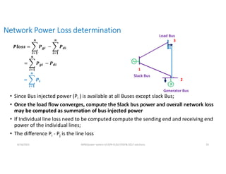
Network Power Lossdetermination
• Since Bus injected power (Pi ) is available at all Buses except slack Bus;
• Once the load flow converges, compute the Slack bus power and overall network loss
may be computed as summation of bus injected power
• If Individual line loss need to be computed compute the sending end and receiving end
power of the individual lines;
• The difference Pi - Pj is the line loss
6/16/2021 AKM/power system-ii/L9/N-R,DLF,FDLF& DCLF solutions 10
𝑷𝒍𝒐𝒔𝒔 = 𝑷𝒈𝒊
𝒏
𝒊 𝟏
− 𝑷𝒅𝒊
𝒏
𝒊 𝟏
= 𝑷𝒈𝒊
𝒏
𝒊 𝟏
− 𝑷𝒅𝒊
= 𝑷𝒊
𝒏
𝒊 𝟏
1
2
3
Slack Bus
Generator Bus
Load Bus
95.
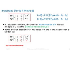
Important: (For N-RMethod)
• In the Jacobean Matrix, The elements with derivative of V has less
multiple of V than the elements with derivative δ
• Hence often an additional V is multiplied to J2 and J4 and the equation is
written like;
6/16/2021 AKM/power system-ii/L9/N-R,DLF,FDLF& DCLF solutions 11
V
V
|Δ𝑉|
𝑽
Don’t confuse with literatures
𝒊= 𝒊 𝒋 𝒊𝒋 𝒊 𝒋
𝒏
𝒋 𝟏 𝒊𝒋
𝒊= 𝒊 𝒋 𝒊𝒋 𝒊 𝒋
𝒏
𝒋 𝟏 𝒊𝒋
96.
Arbind K. Mishra
IOE,Pulchowk Campus
6/21/2021 AKM/power system-ii/L10/Power System Fault calculations
1
D1
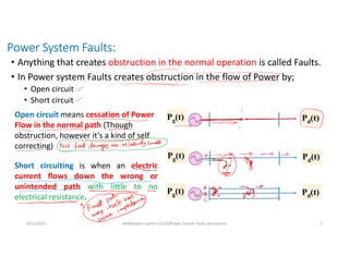
Power System Faults:
•Anything that creates obstruction in the normal operation is called Faults.
• In Power system Faults creates obstruction in the flow of Power by;
• Open circuit
• Short circuit
6/21/2021 AKM/power system-ii/L10/Power System Fault calculations 2
Open circuit means cessation of Power
Flow in the normal path (Though
obstruction, however it’s a kind of self
correcting)
Short circuiting is when an electric
current flows down the wrong or
unintended path with little to no
electrical resistance.
Pg(t) Pd(t)
Pg(t) Pd(t)
Pg(t) Pd(t)
99.
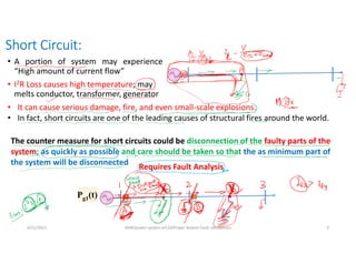
Short Circuit:
• Aportion of system may experience
“High amount of current flow”
• I2R Loss causes high temperature; may
melts conductor, transformer, generator
6/21/2021 AKM/power system-ii/L10/Power System Fault calculations 3
The counter measure for short circuits could be disconnection of the faulty parts of the
system; as quickly as possible and care should be taken so that the as minimum part of
the system will be disconnected
• It can cause serious damage, fire, and even small-scale explosions.
• In fact, short circuits are one of the leading causes of structural fires around the world.
Pg1(t)
Requires Fault Analysis
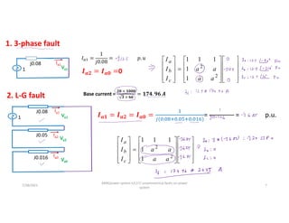
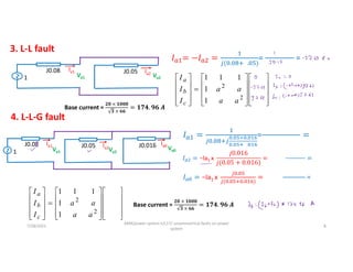
100.
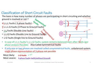
Classification of ShortCircuit Faults
• L-L-L Faults ( 3 phase Faults)
• L-L-L-G Faults (3 Phase to Ground Faults)
• L-L Faults (Double Line Faults)
• L-L-G Faults (Double Line to Ground Faults)
• L-G Faults (Single line to Ground Faults)
6/21/2021 AKM/power system-ii/L10/Power System Fault calculations 4
The basis is how many number of phases are participating in short circuiting and whether
ground is involved or not ?
• In case of L-L-L Faults/ L-L-L-G Faults; system remains balanced even after Faults (per
phase analysis Possible)
Most likely:
Most severe:
L-G Faults
3-phase Faults (with/without Ground)
Also Called Symmetrical Faults
• If only one or two phases are involved called unsymmetrical faults, unbalanced system,
single phase representation of 3-phase not possible
101.
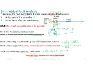
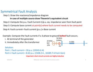
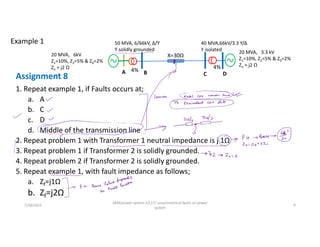
Symmetrical Fault Analysis
•Compute the Fault currents if a 3-phase to ground bolted fault occurs;
i. At terminal of the generator
ii. Immediately after the transformer
6/21/2021 AKM/power system-ii/L10/Power System Fault calculations 5
20 MVA
6kV
10%
50 MVA
6/66kV
4%
X=30Ω
Solution: i. if fault occurs at terminal of the generator
Step 1: Draw the reactance/impedance diagram
Step 2: Compute the p.u. Fault Current=1/p.u. eq. impedance seen from fault point
Step 3: Compute base current at point(s) where fault current needs to be computed
Step 4: Fault current= Fault current (p.u.) x Base current
In case of multiple source draw Thevenin’s equivalent circuit
Important: short circuit currents are highly inductive
102.
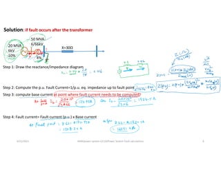
Solution: if faultoccurs after the transformer
6/21/2021 AKM/power system-ii/L10/Power System Fault calculations 6
20 MVA
6kV
10%
50 MVA
6/66kV
4%
X=30Ω
Step 1: Draw the reactance/impedance diagram
Step 2: Compute the p.u. Fault Current=1/p.u. eq. impedance up to fault point
Step 3: compute base current at point where fault current needs to be computed
Step 4: Fault current= Fault current (p.u.) x Base current
103.
Arbind K. Mishra
IOE,Pulchowk Campus
6/28/2021 AKM/power system-ii/L11/ Faults & unbalance system
1
D1
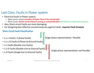
Last Class: Faultsin Power system
• L-L-L Faults ( 3 phase Faults)
• L-L-L-G Faults (3 Phase to Ground Faults)
• L-L Faults (Double Line Faults)
• L-L-G Faults (Double Line to Ground Faults)
• L-G Faults (Single line to Ground Faults)
6/28/2021 AKM/power system-ii/L11/ Faults & unbalance system 2
Short circuit Fault Classification
Symmetrical
Faults
Unsymmetrical
Faults
• Electrical Faults In Power system;
• Open circuit: means cessation of Power Flow in the normal path
• Short circuit: electric current flows in wrong or unintended path with little to no electrical resistance
• Also; Short circuit Faults are more damaging;
• For designing best effective countermeasures against Faults requires Fault Analysis
Single phase representation Possible
Single phase representation not Possible
106.
Symmetrical Fault Analysis
Example:Compute the Fault currents if a 3-phase to ground bolted fault occurs;
i. At terminal of the generator
ii. Immediately after the transformer
6/28/2021 AKM/power system-ii/L11/ Faults & unbalance system 3
20 MVA
6kV
10%
50 MVA
6/66kV
4%
X=30Ω
Step 1: Draw the reactance/impedance diagram
Step 2: Compute the p.u. Fault Current=1/p.u. eq. impedance seen from fault point
Step 3: Compute base current at point(s) where fault current needs to be computed
Step 4: Fault current= Fault current (p.u.) x Base current
In case of multiple source draw Thevenin’s equivalent circuit
Important: short circuit currents are highly inductive
Solution:
Part i.: Fault current = 10 p.u. (19245.6 A)
Part ii: Fault current = 8.62 p.u. (1508.2 A , 16589.7 A from Gen)
107.
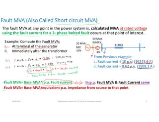
Fault MVA (AlsoCalled Short circuit MVA)
The fault MVA at any point in the power system is, calculated MVA at rated voltage
using the fault current for a 3- phase bolted fault occurs at that point of interest.
6/28/2021 AKM/power system-ii/L11/ Faults & unbalance system 4
20 MVA
6kV
10%
50 MVA
6/66kV
4%
X=30Ω
Example: Compute the Fault MVA;
i. At terminal of the generator
ii. Immediately after the transformer
Fault MVA= Base MVA/equivalent p.u. impedance from source to that point
In p.u. Fault MVA & Fault Current same
From Previous example:
i.: Fault current = 10 p.u. (19245.6 A)
ii: Fault current = 8.62 p.u. (1508.2 A )
Fault MVA= Base MVA* p.u. Fault current
108.
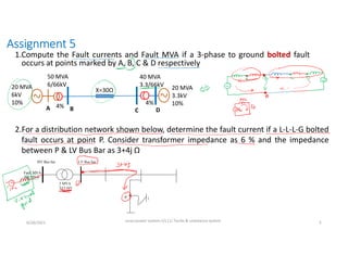
Assignment 5
6/28/2021 AKM/powersystem-ii/L11/ Faults & unbalance system 5
1.Compute the Fault currents and Fault MVA if a 3-phase to ground bolted fault
occurs at points marked by A, B, C & D respectively
20 MVA
6kV
10%
50 MVA
6/66kV
4%
X=30Ω 20 MVA
3.3kV
10%
A B
40 MVA
3.3/66kV
4%
C D
For the distribution Network shown below determines the
fault current if a LLLG fault occurs at point P. Take
transformer impedance as 6% and the impedance between
P and LV bus bar as; 3 + j 4 .
P
3 MVA
33/11kV
Fault MVA
200 MVA
LV Bus bar
HV Bus bar
2.For a distribution network shown below, determine the fault current if a L-L-L-G bolted
fault occurs at point P. Consider transformer impedance as 6 % and the impedance
between P & LV Bus Bar as 3+4j Ω
109.
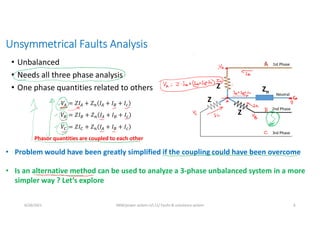
Unsymmetrical Faults Analysis
•Unbalanced
• Needs all three phase analysis
• One phase quantities related to others
6/28/2021 AKM/power system-ii/L11/ Faults & unbalance system 6
𝑉 = 𝑍𝐼 + 𝑍 𝐼 + 𝐼 + 𝐼
𝑉 = 𝑍𝐼 + 𝑍 𝐼 + 𝐼 + 𝐼
𝑉 = 𝑍𝐼 + 𝑍 𝐼 + 𝐼 + 𝐼
Z
Z
Z
Zn
• Problem would have been greatly simplified if the coupling could have been overcome
• Is an alternative method can be used to analyze a 3-phase unbalanced system in a more
simpler way ? Let’s explore
Phasor quantities are coupled to each other
110.
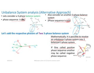
Unbalance System analysis(Alternative Approach)
• Lets consider a 3-phase balance system
• phase sequence is abc
6/28/2021 AKM/power system-ii/L11/ Faults & unbalance system 7
Mathematically, It is possible to resolve
an unbalance 3 phase system into 2
balanced 3 phase system
If One called positive
phase sequence another
may be called negative
phase sequence
Let’s add the respective phasors of Two 3-phase balance system
• Also consider an another 3 phase balance
system
• (Phase sequence is acb)
111.
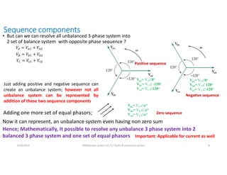
Sequence components
• Butcan we can resolve all unbalanced 3-phase system into
2 set of balance system with opposite phase sequence ?
6/28/2021 AKM/power system-ii/L11/ Faults & unbalance system 8
Hence; Mathematically, It possible to resolve any unbalance 3 phase system into 2
balanced 3 phase system and one set of equal phasors
𝑉 = 𝑉 + 𝑉
𝑉 = 𝑉 + 𝑉
𝑉 = 𝑉 + 𝑉
Vao= V0 o
Vbo= V0 o
Vco= V0 o
Just adding positive and negative sequence can
create an unbalance system; however not all
unbalance system can be represented by
addition of these two sequence components
Adding one more set of equal phasors;
Now it can represent, an unbalance system even having non zero sum
Va1= V10o
Vb1= V1 -120o
Vc1= V1 120o
Va2= V20o
Vb2= V2 120o
Vc2= V2 -120o
Zero sequence
Positive sequence
Negative sequence
Important: Applicable for current as well
112.
6/28/2021
AKM/power system-ii/L11/ Faults& unbalance
system
9
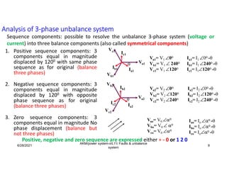
Analysis of 3-phase unbalance system
1. Positive sequence components: 3
components equal in magnitude
displaced by 1200 with same phase
sequence as for original (balance
three phases)
2. Negative sequence components: 3
components equal in magnitude
displaced by 1200 with opposite
phase sequence as for original
(balance three phases)
3. Zero sequence components: 3
components equal in magnitude No
phase displacement (balance but
not three phases)
Sequence components: possible to resolve the unbalance 3-phase system (voltage or
current) into three balance components (also called symmetrical components)
Va1
Vc1
Vb1
Ia1
Ic1
Ib1
Va1= V1 0o
Vb1= V1 240o
Vc1= V1 120o
Ia1= I1 0o -
Ib1= I1 240o -
Ic1= I1120o -
Va2= V2 0o
Vb2= V2 120o
Vc2= V2 240o
Va2
Vb2
Vc2
Ia2
Ib2
Ic2
Ia2= I2 0o -
Ib2= I2 120o -
Ic2= I2 240o -
Vao= V0 o
Vbo= V0 o
Vco= V0 o
Iao= Io o -
Ibo= Io o -
Ico= Ioo -
Positive, negative and zero sequence are expressed either + - 0 or 1 2 0
113.
Arbind K. Mishra
IOE,Pulchowk Campus
6/28/2021 AKM/power system-ii/L12/ Faults & unbalance system
1
114.
6/28/2021
AKM/power system-ii/L12/ Faults& unbalance
system
2
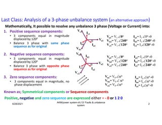
Last Class: Analysis of a 3-phase unbalance system (an alternative approach)
1. Positive sequence components:
• 3 components equal in magnitude
displaced by 1200
• Balance 3 phase with same phase
sequence as for original
2. Negative sequence components:
• 3 components equal in magnitude
displaced by 1200
• Balance 3 phase with opposite phase
sequence as for original
3. Zero sequence components:
• 3 components equal in magnitude, no
phase displacement
Mathematically, It possible to resolve any unbalance 3 phase (Voltage or Current) into:
Va1
Vc1
Vb1
Ia1
Ic1
Ib1
Va1= V1 0o
Vb1= V1 240o
Vc1= V1 120o
Ia1= I1 0o -
Ib1= I1 240o -
Ic1= I1120o -
Va2= V2 0o
Vb2= V2 120o
Vc2= V2 240o
Va2
Vb2
Vc2
Ia2
Ib2
Ic2
Ia2= I2 0o -
Ib2= I2 120o -
Ic2= I2 240o -
Vao= V0 o
Vbo= V0 o
Vco= V0 o
Iao= Io o -
Ibo= Io o -
Ico= Ioo -
Positive, negative and zero sequence are expressed either + - 0 or 1 2 0
Known as; Symmetrical components or Sequence components
115.
6/28/2021
AKM/power system-ii/L12/ Faults& unbalance
system
3
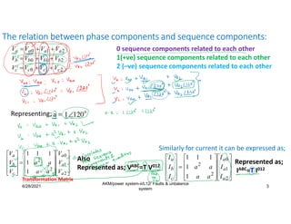
The relation between phase components and sequence components:
Also
Represented as; VABC=T V012
2
1
0
2
2
1
1
1
1
1
a
a
a
c
b
a
I
I
I
a
a
a
a
I
I
I
Represented as;
IABC=T I012
2
1
0 a
a
a
a V
V
V
V
2
1
0 b
b
b
b V
V
V
V
2
1
0 c
c
c
c V
V
V
V
Also; 0
0
0 c
b
a V
V
V
1
1
1
2
1 & a
c
a
b V
V
V
V
1
2
2
1
2 & a
c
a
b V
V
V
V
2
1
0
2
2
1
1
1
1
1
a
a
a
c
b
a
V
V
V
a
a
a
a
V
V
V
Similarly for current it can be expressed as;
Representing;
0 sequence components related to each other
1(+ve) sequence components related to each other
2 (–ve) sequence components related to each other
Transformation Matrix
116.
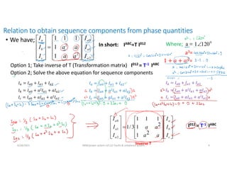
Relation to obtainsequence components from phase quantities
• We have;
6/28/2021 AKM/power system-ii/L12/ Faults & unbalance system 4
In short: IABC=T I012 Where;
Option 1; Take inverse of T (Transformation matrix) I012 = T-1 IABC
Option 2; Solve the above equation for sequence components
c
b
a
a
a
a
I
I
I
a
a
a
a
I
I
I
2
1
2
1
1
1
1
3
/
1
2
1
0
2
1
0
2
2
1
1
1
1
1
a
a
a
c
b
a
I
I
I
a
a
a
a
I
I
I
a3=
=
I012 = T-1 IABC
Inverse T
𝐼 = 𝐼 + 𝐼 + 𝐼
𝐼 = 𝐼 + 𝑎2𝐼 + 𝑎𝐼
𝐼 = 𝐼 + 𝑎𝐼 + 𝑎2𝐼
𝐼 = 𝐼 + 𝐼 + 𝐼
𝐼 = 𝐼 + 𝑎2𝐼 + 𝑎𝐼
𝐼 = 𝐼 + 𝑎𝐼 + 𝑎2𝐼
𝐼 = 𝐼 + 𝐼 + 𝐼
𝐼 = 𝐼 + 𝑎2𝐼 + 𝑎𝐼
𝐼 = 𝐼 + 𝑎𝐼 + 𝑎2𝐼
117.
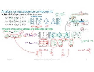
Analysis using sequencecomponents
• Recall the 3-phase unbalance system
6/28/2021 AKM/power system-ii/L12/ Faults & unbalance system 5
𝑉 = 𝑍𝐼 + 𝑍 𝐼 + 𝐼 + 𝐼
𝑉 = 𝑍𝐼 + 𝑍 𝐼 + 𝐼 + 𝐼
𝑉 = 𝑍𝐼 + 𝑍 𝐼 + 𝐼 + 𝐼
Z
Z
Z
Zn
In terms of sequence voltage and sequence currents
𝑽𝑨
𝑽𝑩
𝑽𝑪
=
𝒁 + 𝒁𝒏 𝒁𝒏 𝒁𝒏
𝒁𝒏 𝒁 + 𝒁𝒏 𝒁𝒏
𝒁𝒏 𝒁𝒏 𝒁 + 𝒁𝒏
𝑰𝑨
𝑰𝑩
𝑰𝑪
In Matrix Form
T V012 = ZABC T I012
V012 = T-1 ZABC T I012
T-1 ZABCT T =
1
3
1 1 1
1 𝑎 𝑎
1 𝑎 𝑎
𝒁 + 𝒁𝒏 𝒁𝒏 𝒁𝒏
𝒁𝒏 𝒁 + 𝒁𝒏 𝒁𝒏
𝒁𝒏 𝒁𝒏 𝒁 + 𝒁𝒏
1 1 1
1 𝑎 𝑎
1 𝑎 𝑎
VABC = ZABC IABC
1
3
1 1 1
1 𝑎 𝑎
1 𝑎 𝑎
T-1 ZABCT T =
118.
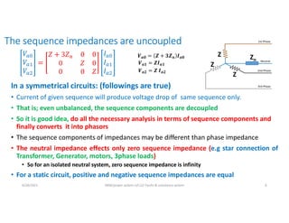
The sequence impedancesare uncoupled
In a symmetrical circuits: (followings are true)
• Current of given sequence will produce voltage drop of same sequence only.
• That is; even unbalanced, the sequence components are decoupled
• So it is good idea, do all the necessary analysis in terms of sequence components and
finally converts it into phasors
• The sequence components of impedances may be different than phase impedance
• The neutral impedance effects only zero sequence impedance (e.g star connection of
Transformer, Generator, motors, 3phase loads)
• So for an isolated neutral system, zero sequence impedance is infinity
• For a static circuit, positive and negative sequence impedances are equal
6/28/2021 AKM/power system-ii/L12/ Faults & unbalance system 6
𝑽𝒂𝟎 = 𝒁 + 𝟑𝒁𝒏 𝑰𝒂𝟎
𝑽𝒂𝟏 = 𝒁𝑰𝒂𝟏
𝑽𝒂𝟐 = 𝒁 𝑰𝒂𝟐
Z
Z
Z
Zn
119.
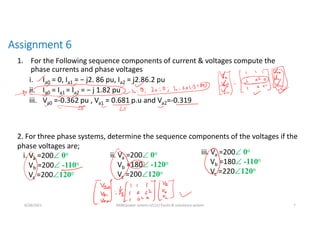
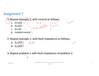
Assignment 6
1. Forthe Following sequence components of current & voltages compute the
phase currents and phase voltages
i. Ia0 = 0, Ia1 = − j2. 86 pu, Ia2 = j2.86.2 pu
ii. Ia0 = Ia1 = Ia2 = − j 1.82 pu
iii. Va0 =-0.362 pu , Va1 = 0.681 p.u and Va2=-0.319
6/28/2021 AKM/power system-ii/L12/ Faults & unbalance system 7
i. Va =200 0o
Vb =200 -110o
Vc =200120o
ii. Va =200 0o
Vb =180 -120o
Vc =200120o
iii. Va =200 0o
Vb =180 -110o
Vc =220120o
2. For three phase systems, determine the sequence components of the voltages if the
phase voltages are;
120.
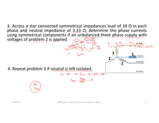
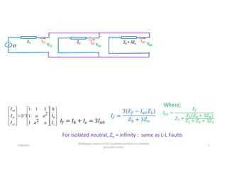
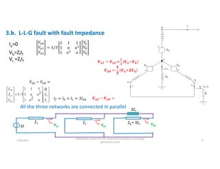
3. Across astar connected symmetrical impedances load of 10 Ω in each
phase and neutral impedance of 3.33 Ω, determine the phase currents
using symmetrical components if an unbalanced three phase supply with
voltages of problem 2 is applied.
6/28/2021 AKM/power system-ii/L12/ Faults & unbalance system 8
4. Repeat problem 3 if neutral is left isolated.
Z
Z
Z
Zn
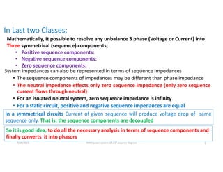
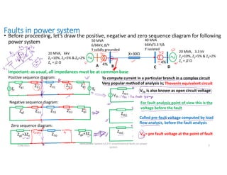
In Last twoClasses;
System impedances can also be represented in terms of sequence impedances
• The sequence components of impedances may be different than phase impedance
• The neutral impedance effects only zero sequence impedance (only zero sequence
current flows through neutral)
• For an isolated neutral system, zero sequence impedance is infinity
• For a static circuit, positive and negative sequence impedances are equal
7/28/2021 AKM/power system-ii/L13/ sequnce diagram 2
Mathematically, It possible to resolve any unbalance 3 phase (Voltage or Current) into
Three symmetrical (sequence) components;
• Positive sequence components:
• Negative sequence components:
• Zero sequence components:
In a symmetrical circuits Current of given sequence will produce voltage drop of same
sequence only. That is; the sequence components are decoupled
So it is good idea, to do all the necessary analysis in terms of sequence components and
finally converts it into phasors
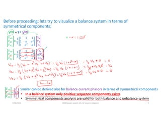
123.
Before proceeding; letstry to visualize a balance system in terms of
symmetrical components;
V012 = T-1 VABC
1
3
1 1 1
1 𝑎 𝑎
1 𝑎 𝑎
𝑉
𝑉
𝑉
=
𝑉
𝑉
𝑉
1
3
1 1 1
1 𝑎 𝑎
1 𝑎 𝑎
𝑉
𝑉
𝑉
=
𝑉
α2𝑉
α𝑉
𝑉
𝑉
𝑉
=
0
𝑉
0
• In a balance system only positive sequence components exists
• Symmetrical components analysis are valid for both balance and unbalance system
Similar can be derived also for balance current phasors in terms of symmetrical components
7/28/2021 AKM/power system-ii/L13/ sequnce diagram 3
124.
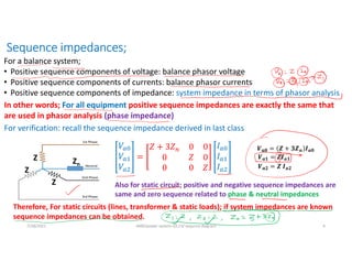
Sequence impedances;
For abalance system;
• Positive sequence components of voltage: balance phasor voltage
• Positive sequence components of currents: balance phasor currents
• Positive sequence components of impedance: system impedance in terms of phasor analysis
In other words; For all equipment positive sequence impedances are exactly the same that
are used in phasor analysis (phase impedance)
For verification; recall the sequence impedance derived in last class
Z
Z
Z
Zn
𝑽𝒂𝟎 = 𝒁 + 𝟑𝒁𝒏 𝑰𝒂𝟎
𝑽𝒂𝟏 = 𝒁𝑰𝒂𝟏
𝑽𝒂𝟐 = 𝒁 𝑰𝒂𝟐
Also for static circuit; positive and negative sequence impedances are
same and zero sequence related to phase & neutral impedances
Therefore, For static circuits (lines, transformer & static loads); if system impedances are known
sequence impedances can be obtained.
7/28/2021 AKM/power system-ii/L13/ sequnce diagram 4
125.
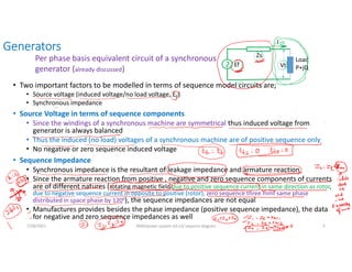
Generators
• Two importantfactors to be modelled in terms of sequence model circuits are;
• Source voltage (induced voltage/no load voltage, Ef )
• Synchronous impedance
• Source Voltage in terms of sequence components
• Since the windings of a synchronous machine are symmetrical thus induced voltage from
generator is always balanced
• Thus the induced (no load) voltages of a synchronous machine are of positive sequence only
• No negative or zero sequence induced voltage
• Sequence Impedance
• Synchronous impedance is the resultant of leakage impedance and armature reaction
• Since the armature reaction from positive , negative and zero sequence components of currents
are of different natures (rotating magnetic field due to positive sequence current in same direction as rotor,
due to negative sequence current in opposite to positive (rotor), zero sequence three mmf same phase
distributed in space phase by 1200), the sequence impedances are not equal
• Manufactures provides besides the phase impedance (positive sequence impedance), the data
for negative and zero sequence impedances as well
Ef
Zs
Load
P+jQ
Vt
I
Per phase basis equivalent circuit of a synchronous
generator (already discussed)
7/28/2021 AKM/power system-ii/L13/ sequnce diagram 5
126.
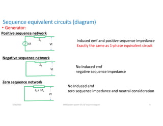
Sequence equivalent circuits(diagram)
• Generator:
Ef
Z1
Vt
Positive sequence network
Induced emf and positive sequence impedance
Exactly the same as 1-phase equivalent circuit
Negative sequence network
Z2
Vt
No Induced emf
negative sequence impedance
Z0 + 3Zn
Vt
No Induced emf
zero sequence impedance and neutral consideration
Zero sequence network
7/28/2021 AKM/power system-ii/L13/ sequnce diagram 6
127.
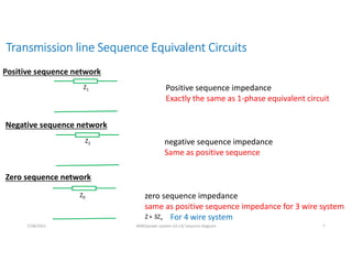
Transmission line SequenceEquivalent Circuits
Z1
Positive sequence network
Positive sequence impedance
Exactly the same as 1-phase equivalent circuit
Negative sequence network
Z2 negative sequence impedance
Same as positive sequence
Z0
Zero sequence network
zero sequence impedance
same as positive sequence impedance for 3 wire system
For 4 wire system
Z+ 3Zn
7/28/2021 AKM/power system-ii/L13/ sequnce diagram 7
128.
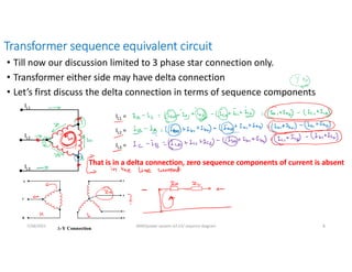
Transformer sequence equivalentcircuit
• Till now our discussion limited to 3 phase star connection only.
• Transformer either side may have delta connection
• Let’s first discuss the delta connection in terms of sequence components
IL1
IL2
IL3
IL1 =
IL2 =
IL3 =
That is in a delta connection, zero sequence components of current is absent
7/28/2021 AKM/power system-ii/L13/ sequnce diagram 8
129.
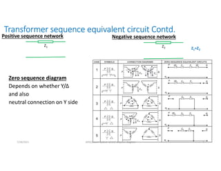
Transformer sequence equivalentcircuit Contd.
Zero sequence diagram
Depends on whether Y/Δ
and also
neutral connection on Y side
Z1
Positive sequence network Negative sequence network
Z2
7/28/2021 AKM/power system-ii/L13/ sequnce diagram 9
Z1=Z2
130.
7/28/2021 AKM/power system-ii/L13/sequnce diagram 10
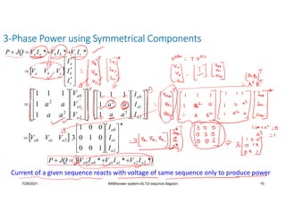
3-Phase Power using Symmetrical Components
Current of a given sequence reacts with voltage of same sequence only to produce power
131.
Arbind K. Mishra
IOE,Pulchowk Campus
7/28/2021
AKM/power system-ii/L14/ unsymmetrical faults on unloaded
generators
1
132.
7/28/2021
AKM/power system-ii/L14/ unsymmetricalfaults
on unloaded generators
2
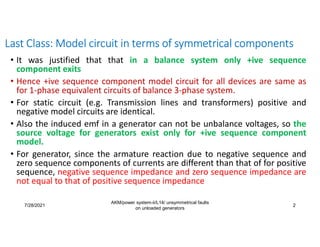
Last Class: Model circuit in terms of symmetrical components
• It was justified that that in a balance system only +ive sequence
component exits
• Hence +ive sequence component model circuit for all devices are same as
for 1-phase equivalent circuits of balance 3-phase system.
• For static circuit (e.g. Transmission lines and transformers) positive and
negative model circuits are identical.
• Also the induced emf in a generator can not be unbalance voltages, so the
source voltage for generators exist only for +ive sequence component
model.
• For generator, since the armature reaction due to negative sequence and
zero sequence components of currents are different than that of for positive
sequence, negative sequence impedance and zero sequence impedance are
not equal to that of positive sequence impedance
133.
7/28/2021
AKM/power system-ii/L14/ unsymmetricalfaults
on unloaded generators
3
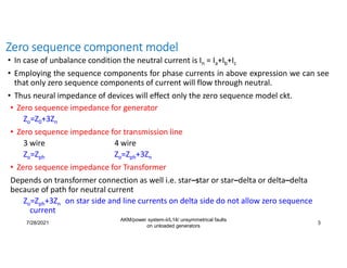
Zero sequence component model
• In case of unbalance condition the neutral current is In = Ia+Ib+Ic
• Employing the sequence components for phase currents in above expression we can see
that only zero sequence components of current will flow through neutral.
• Thus neural impedance of devices will effect only the zero sequence model ckt.
• Zero sequence impedance for generator
Zo=Z0+3Zn
• Zero sequence impedance for transmission line
3 wire 4 wire
Zo=Zph Zo=Zph+3Zn
• Zero sequence impedance for Transformer
Depends on transformer connection as well i.e. star–star or star–delta or delta–delta
because of path for neutral current
Zo=Zph+3Zn on star side and line currents on delta side do not allow zero sequence
current
134.
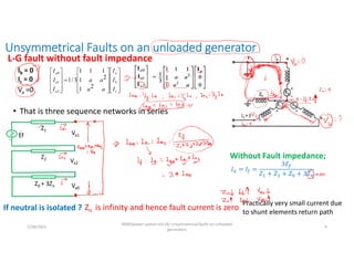
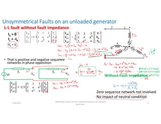
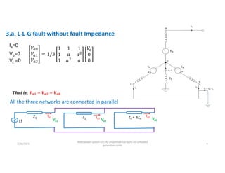
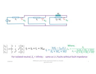
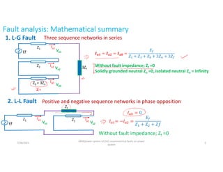
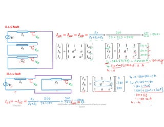
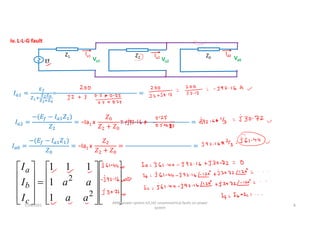
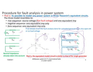
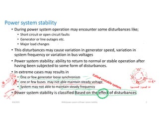
Unsymmetrical Faults onan unloaded generator
• That is three sequence networks in series
Ib = 0
Ic = 0
Ef
Z1
Va1
Z2 Va2
Z0 + 3Zn Va0
If neutral is isolated ?
Without Fault impedance;
𝐼 = 𝐼 =
3𝐸
𝑍 + 𝑍 + 𝑍 + 3𝑍
Zn is infinity and hence fault current is zero
Practically very small current due
to shunt elements return path
L-G fault without fault impedance
Va =0
7/28/2021
AKM/power system-ii/L14/ unsymmetrical faults on unloaded
generators
4
c
b
a
a
a
a
I
I
I
a
a
a
a
I
I
I
2
1
2
1
1
1
1
3
/
1
2
1
0
135.
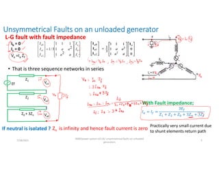
Unsymmetrical Faults onan unloaded generator
• That is three sequence networks in series
Ib = 0
Ic = 0
Ef
Z1
Va1
Z2 Va2
Z0 + 3Zn Va0
If neutral is isolated ?
𝐼 = 𝐼 =
3𝐸
𝑍 + 𝑍 + 𝑍 + 3𝑍 + 3𝑍
With Fault impedance;
Zn is infinity and hence fault current is zero
Practically very small current due
to shunt elements return path
L-G fault with fault impedance
Va =Ia Zf
7/28/2021
AKM/power system-ii/L14/ unsymmetrical faults on unloaded
generators
5
c
b
a
a
a
a
I
I
I
a
a
a
a
I
I
I
2
1
2
1
1
1
1
3
/
1
2
1
0
136.
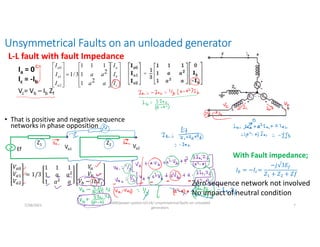
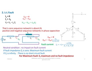
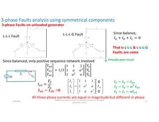
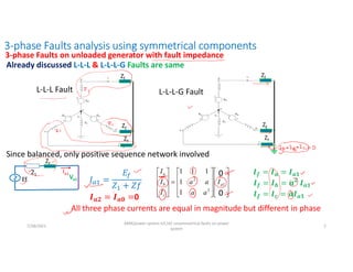
Unsymmetrical Faults onan unloaded generator
• That is positive and negative sequence
networks in phase opposition
Ia = 0
Ic = -Ib
Ef
Z1
Va1
Z2 Va2
Without Fault impedance;
𝐼 = −𝐼 =
−𝑗√3𝐸
𝑍 + 𝑍
L-L fault without fault impedance
Zero sequence network not involved
No impact of neutral condition
𝑉
𝑉
𝑉
= 1/3
1 1 1
1 𝑎 𝑎
1 𝑎 𝑎
𝑉
𝑉
𝑉
Vb = Vc
7/28/2021
AKM/power system-ii/L14/ unsymmetrical faults on unloaded
generators
6
c
b
a
a
a
a
I
I
I
a
a
a
a
I
I
I
2
1
2
1
1
1
1
3
/
1
2
1
0
137.
Unsymmetrical Faults onan unloaded generator
• That is positive and negative sequence
networks in phase opposition
Ia = 0
Ic = -Ib
Ef
Z1
Va1
Z2 Va2
With Fault impedance;
𝐼 = −𝐼 =
−𝑗√3𝐸
𝑍 + 𝑍 + 𝑍𝑓
L-L fault with fault Impedance
𝑉
𝑉
𝑉
= 1/3
1 1 1
1 𝑎 𝑎
1 𝑎 𝑎
𝑉
𝑉
𝑉 − 𝐼𝑏𝑍𝑓
Vc= Vb – Ib Zf
7/28/2021
AKM/power system-ii/L14/ unsymmetrical faults on unloaded
generators
7
Zero sequence network not involved
No impact of neutral condition
c
b
a
a
a
a
I
I
I
a
a
a
a
I
I
I
2
1
2
1
1
1
1
3
/
1
2
1
0
138.
Arbind K. Mishra
IOE,Pulchowk Campus
7/28/2021
AKM/power system-ii/L14/ unsymmetrical faults on unloaded
generators contd
1
139.
Last Class: UnsymmetricalFaults on an unloaded generator
That is three sequence networks in series
Ib = 0
Ic = 0
For isolated neutral, Zn = infinity : No fault current (ideally)
𝐼 = 𝐼 =
3𝐸
𝑍 + 𝑍 + 𝑍 + 3𝑍 + 3𝑍
Fault Current;
1. L-G Fault
Va =Ia Zf
7/28/2021
AKM/power system-ii/L14/ unsymmetrical faults on unloaded
generators contd
2
𝑰𝒂𝟏 = 𝑰𝒂𝟐 = 𝑰𝒂𝟎 =
𝟏
𝟑
𝑰𝒂
𝑽𝒂𝟎 + 𝑽𝒂𝟏 + 𝑽𝒂𝟐 = 𝟑𝑰𝒂𝟏𝒁𝒇
Z2 Va2
Ia2
Ef
Z1
Va1
Ia1
Z0 + 3Zn Va0
Ia0
3Zf
For solidly grounded neutral, Zn = 0 : fault current maximum
If Zf is infinity : There is no short circuit fault
If Zf is zero(Without fault impedance): Maximum fault current
For Maximum Fault: Ef maximum, solidly grounded neutral, no fault impedance
𝑰𝒂𝟏 = 𝑰𝒂𝟐 = 𝑰𝒂𝟎 =
𝐸
𝑍 + 𝑍 + 𝑍 + 3𝑍 + 3𝑍
140.
That is zerosequence network is absent &
positive and negative sequence networks in phase opposition
Ia = 0
Ic = -Ib
Fault current 𝐼 = −𝐼 =
−𝑗√3𝐸
𝑍 + 𝑍 + 𝑍𝑓
2. L-L Fault
Vc= Vb – Ib Zf
7/28/2021
AKM/power system-ii/L14/ unsymmetrical faults on unloaded
generators contd
3
𝑰𝒂𝟎 = 𝟎
𝑰𝒂𝟏= −𝑰𝒂𝟐
𝑽𝒂𝟏 − 𝑽𝒂𝟐 = 𝑰𝒂𝟏𝒁𝒇
Ef
Z1
Va1
Ia1 Z2
Va2
Ia2
Zf
Neutral condition : no impact on fault current
If Zf is infinity : There is no short circuit fault
If fault impedance Zf is zero: Maximum fault current
For Maximum Fault: Ef maximum and no fault impedance
𝑰𝒂𝟎 = 𝟎
𝑰𝒂𝟏= −𝑰𝒂𝟐=
141.
7/28/2021
AKM/power system-ii/L14/ unsymmetricalfaults on unloaded
generators contd
4
3.a. L-L-G fault without fault Impedance
Ia=0
Vb=0
Vc =0
𝑻𝒉𝒂𝒕 𝒊𝒔; 𝑽𝒂𝟏 = 𝑽𝒂𝟐 = 𝑽𝒂𝟎
Ef
Z1
Va1
Ia1 Z2
Va2
Ia2 Z0 + 3Zn Va0
Ia0
All the three networks are connected in parallel
142.
7/28/2021
AKM/power system-ii/L14/ unsymmetricalfaults on unloaded
generators contd
5
Ef
Z1
Va1
Ia1 Z2
Va2
Ia2 Z0 + 3Zn Va0
Ia0
c
b
a
a
a
a
I
I
I
a
a
a
a
I
I
I
2
1
2
1
1
1
1
3
/
1
2
1
0 0
For isolated neutral, Zn = infinity : same as L-L Faults
Where;
𝐼 =
𝐸
𝑍 +
𝑍 (𝑍 + 3𝑍 )
𝑍 + 𝑍 + 3𝑍
143.
7/28/2021
AKM/power system-ii/L14/ unsymmetricalfaults on unloaded
generators contd
6
3.b. L-L-G fault with fault Impedance
Ia=0
Vb=ZfIf
Vc =ZfIf
𝑉
𝑉
𝑉
= 1/3
1 1 1
1 𝑎 𝑎
1 𝑎 𝑎
𝑉
𝑉
𝑉
𝑽𝒂𝟏 = 𝑽𝒂𝟐=
𝟏
𝟑
(𝑽𝒂−𝑽𝒃)
𝑽𝒂𝟎 =
𝟏
𝟑
(𝑽𝒂+𝟐𝑽𝒃)
Ef
Z1
Va1
Ia1 Z2
Va2
Ia2 Z0 + 3Zn Va0
Ia0
All the three networks are connected in parallel
𝑉 − 𝑉 =
3Zf
c
b
a
a
a
a
I
I
I
a
a
a
a
I
I
I
2
1
2
1
1
1
1
3
/
1
2
1
0 0
𝐼 = 𝐼 + 𝐼 = 3𝐼 𝑽𝒂𝟐 − 𝑽𝒂𝟎 =
144.
7/28/2021
AKM/power system-ii/L14/ unsymmetricalfaults on unloaded
generators contd
7
Ef
Z1
Va1
Ia1 Z2
Va2
Ia2 Z0 + 3Zn Va0
Ia0
3Zf
c
b
a
a
a
a
I
I
I
a
a
a
a
I
I
I
2
1
2
1
1
1
1
3
/
1
2
1
0 0
For isolated neutral, Zn = infinity : same as L-L Faults without fault impedance
Where;
𝐼 =
𝐸
𝑍 +
𝑍 (𝑍 + 3𝑍 + 3𝑍𝑓)
𝑍 + 𝑍 + 3𝑍 + 3𝑍𝑓
145.
3-phase Faults analysisusing symmetrical components
7/28/2021
AKM/power system-ii/L14/ unsymmetrical faults on unloaded
generators contd
8
L-L-L Fault L-L-L-G Fault Since balance,
That is L-L-L & L-L-L-G
Faults are same
Ef
Z1
Va1
Ia1
Since balanced, only positive sequence network involved
𝒂𝟐 𝒂𝟎 0
2
1
0
2
2
1
1
1
1
1
a
a
a
c
b
a
I
I
I
a
a
a
a
I
I
I 0
0
All three phase currents are equal in magnitude but different in phase
𝒇 𝒂 𝒂𝟏
𝒇 𝒃
𝟐
𝒂𝟏
𝒇 𝒄 𝒂𝟏
Virtually open circuit
3-phase Faults on unloaded generator
146.
Arbind K. Mishra
IOE,Pulchowk Campus
7/28/2021
AKM/power system-ii/L16/ unsymmetrical faults on power
system
1
147.
3-phase Faults analysisusing symmetrical components
7/28/2021
AKM/power system-ii/L16/ unsymmetrical faults on power
system
2
L-L-L Fault L-L-L-G Fault
Already discussed L-L-L & L-L-L-G Faults are same
Since balanced, only positive sequence network involved
𝒂𝟐 𝒂𝟎 0
2
1
0
2
2
1
1
1
1
1
a
a
a
c
b
a
I
I
I
a
a
a
a
I
I
I 0
0
All three phase currents are equal in magnitude but different in phase
𝒇 𝒂 𝒂𝟏
𝒇 𝒃
𝟐
𝒂𝟏
𝒇 𝒄 𝒂𝟏
3-phase Faults on unloaded generator with fault impedance
Zf
Zf
Zf
Ef
Z1
Va1
Ia1
Zf
Zf
Zf
Zf
148.
Fault analysis: Mathematicalsummary
Three sequence networks in series
1. L-G Fault
7/28/2021
AKM/power system-ii/L16/ unsymmetrical faults on power
system
3
Z2 Va2
Ia2
Ef
Z1
Va1
Ia1
Z0 + 3Zn Va0
Ia0
3Zf
𝑰𝒂𝟏 = 𝑰𝒂𝟐 = 𝑰𝒂𝟎 =
𝐸
𝑍 + 𝑍 + 𝑍 + 3𝑍 + 3𝑍
Without fault impedance; Zf =0
Solidly grounded neutral Zn =0, isolated neutral Zn = infinity
2. L-L Fault
Ef
Z1
Va1
Ia1 Z2
Va2
Ia2
Zf
𝐼 = 0
𝐼 = −𝐼 =
𝐸
𝑍 + 𝑍 + 𝑍𝑓
Positive and negative sequence networks in phase opposition
Without fault impedance; Zf =0
149.
7/28/2021
AKM/power system-ii/L16/ unsymmetricalfaults on power
system
4
Ef
Z1
Va1
Ia1 Z2 Va2
Ia2 Z0 + 3Zn Va0
Ia0
3Zf
𝐼 =
( )
= -Ia1 x
𝐼 =
𝐸
𝑍 +
𝑍 (𝑍 + 3𝑍 + 3𝑍𝑓)
𝑍 + 𝑍 + 3𝑍 + 3𝑍𝑓
𝐼 =
( )
= -Ia1 x
3. L-L-G Fault All the three networks are connected in parallel
Without fault impedance; Zf =0
Solidly grounded neutral Zn =0, isolated neutral Zn = infinity
4. Three-Phase Fault
Ef
Z1
Va1
Ia1
Zf
𝒂𝟐 𝒂𝟎 0 Without fault impedance; Zf =0
Only positive sequence network involved
150.
For all typesof Faults
• Phase Currents
2
1
0
2
2
1
1
1
1
1
a
a
a
c
b
a
I
I
I
a
a
a
a
I
I
I
• For phase Voltage
Ef
Z1
Va1
Ia1
Z2
Va2
Ia2
Z0 + 3Zn Va0
Ia0
𝑉 = 𝐸 − 𝐼 𝑍
𝑉 = −𝐼 𝑍
𝑉 = −𝐼 (𝑍 + 3𝑍 )
For isolated neutral
𝒂𝟎 ∞ Indeterminate form
For such case Zero sequence voltage Is determined from
Correlations with other sequence voltage
2
1
0
2
2
1
1
1
1
1
a
a
a
c
b
a
V
V
V
a
a
a
a
V
V
V
7/28/2021
AKM/power system-ii/L16/ unsymmetrical faults on power
system
5
151.
Example 1:
A solidlygrounded 3-phase synchronous generator with generated line to
line voltage of √3 x 200 V is subjected to various types of symmetrical &
unsymmetrical Faults. The sequence impedances of the generator are;
Z1=j2Ω, Z2=j.5Ω & Z0=j0.25Ω. Determine the fault currents.
Solution:
i. 3-phase fault
Ef
Z1
Va1
Ia1
………
= 𝒂𝟐 𝒂𝟎 0
2
1
0
2
2
1
1
1
1
1
a
a
a
c
b
a
I
I
I
a
a
a
a
I
I
I
2
1
0
2
2
1
1
1
1
1
a
a
a
c
b
a
I
I
I
a
a
a
a
I
I
I
7/28/2021
AKM/power system-ii/L16/ unsymmetrical faults on power
system
6
152.
ii. L-G fault
Z2Va2
Ia2
Ef
Z1
Va1
Ia1
Z0 Va0
Ia0
𝒂𝟏 𝒂𝟐 𝒂𝟎 =
………………………………………
=
2
1
0
2
2
1
1
1
1
1
a
a
a
c
b
a
I
I
I
a
a
a
a
I
I
I
iii. L-L fault
Ef
Z1
Va1
Ia1 Z2
Va2
Ia2
=
………………………
=
2
1
0
2
2
1
1
1
1
1
a
a
a
c
b
a
I
I
I
a
a
a
a
I
I
I
2
1
0
2
2
1
1
1
1
1
a
a
a
c
b
a
I
I
I
a
a
a
a
I
I
I
7/28/2021
AKM/power system-ii/L16/ unsymmetrical faults on power
system
7
153.
iv. L-L-G fault
Ef
Z1
Va1
Ia1Z2
Va2
Ia2 Z0 Va0
Ia0
𝐼 = =
…………………………………………………………
=
𝐼 =
−(𝐸 − 𝐼 𝑍 )
𝑍
= −Ia1 x
𝑍
𝑍 + 𝑍
… … … … … … … … … … … .
=
𝐼 =
−(𝐸 − 𝐼 𝑍 )
𝑍
= −Ia1 x
𝑍
𝑍 + 𝑍
=
… … … … … … … … … … …
=
2
1
0
2
2
1
1
1
1
1
a
a
a
c
b
a
I
I
I
a
a
a
a
I
I
I
7/28/2021
AKM/power system-ii/L16/ unsymmetrical faults on power
system
8
154.
Assignment 7
1. Repeatexample 1, with neutral as follows;
a. Zn=j2Ω
b. Zn=j5Ω
c. Zn=2Ω
d. Isolated neutral
2. Repeat example 1, with fault impedance as follows;
a. Zf=j1Ω
b. Zf=j2Ω
3. Repeat problem 1 with fault impedance of problem 2.
7/28/2021
AKM/power system-ii/L16/ unsymmetrical faults on power
system
9
155.
Arbind K. Mishra
IOE,Pulchowk Campus
7/28/2021
AKM/power system-ii/L17/ unsymmetrical faults on power
system
1
156.
Faults in powersystem
• Before proceeding, let’s draw the positive, negative and zero sequence diagram for following
power system
Important: as usual, all impedances must be at common base
20 MVA, 6kV
Z1=10%, Z2=5% & Z0=2%
Zn = j2 Ω
50 MVA
6/66kV, Δ/Y
Y solidly grounded
4%
X=30Ω
A B
40 MVA
66kV/3.3 Y/Δ
Y isolated
4%
C D
20 MVA, 3.3 kV
Z1=10%, Z2=5% & Z0=2%
Zn = j2 Ω
Positive sequence diagram:
ZTr1 ZTl1 ZTr1
Zg1
Ef
Zg1
Ef
Zg2 ZTr2 ZTl2 ZTr2
Zg2
Zg0+3Zn ZTl0
Zg0+3Zn
To compute current in a particular branch in a complex circuit
Very popular method of analysis is; Thevenin equivalent circuit
Zth1
Vth
Zth2
Zth0
VTh is also known as open circuit voltage
For fault analysis point of view this is the
voltage before the fault
Called pre-fault voltage computed by load
flow analysis, before the fault analysis
Negative sequence diagram:
Zero sequence diagram:
7/28/2021
AKM/power system-ii/L17/ unsymmetrical faults on power
system
2
Vth= pre fault voltage at the point of fault
157.
7/28/2021
AKM/power system-ii/L17/ unsymmetricalfaults
on power system
3
Procedure for fault analysis in power system
• That is: its possible to model any power system as three Thevenin’s equivalent circuits.
The three model resembles to:
• +ive sequence: source voltage (Pre-fault voltage) and one equivalent imp
• negative sequence: one equivalent imp only
• Zero sequence: one equivalent imp only
Zth1
Voc
Zth2
Zth0
If we deeply recall the fault analysis done for unloaded generator Ef is also open ckt
or no load voltage
Z2 Va2
Ia2
Ef
Z1
Va1
Ia1
Z0 + 3Zn Va0
Ia0
That is, the equivalent model circuit is similar to that of for single generator
Neutral impedance
already taken into account
158.
Overall procedure
• Drawthe three sequence model circuits for whole system.
• Locate the fault location
• Evaluate the Thieveries equivalent ckt for each sequence ckts corresponding to
fault location.
• Imp: no consideration till now for fault type
• Now based on fault types connect the equivalent sequence networks
appropriately
• L-G Faults: all three networks in series
• L-L Faults : positive and negative sequence in phase opposition
• L-L-G Faults: all three networks in parallel
• 3-phase Faults: only positive sequence network
• Compute the sequence components of currents from the model circuits
• Convert the sequence components of currents to phase currents using
transformation matrix.
2
1
0
2
2
1
1
1
1
1
a
a
a
c
b
a
I
I
I
a
a
a
a
I
I
I
7/28/2021
AKM/power system-ii/L17/ unsymmetrical faults on power
system
4
159.
Example1:
For the powersystem network shown below compute the fault currents if various types of
faults occur at point B. Assume voltage at the point of fault before fault is 1 p.u
First convert all the per unit impedances at common base;
Let’s take generator 1 as common base;
For generator1 ;
Z1=10%, Z2=5% & Z0=2%
Zn = j2 Ω
Base impedance;
6
20
=
𝑍 =
𝑗2
1.8
= 𝑗 𝑝. 𝑢
For Transformer1 ;
Old base; =
6
50
=
New base; =
6
20
=
Z p.u. (new)
= 𝑍(𝑜𝑙𝑑)
𝑍 (𝑜𝑙𝑑)
𝑍 (𝑛𝑒𝑤)
=j.04 x
.
.
=j
For Transmission line;
Zbase; =
66
20
=
Z p.u. = 𝒁
𝒁𝒃𝒂𝒔𝒆
Z p.u. = 𝒋𝟑𝟎
𝟐𝟏𝟕.𝟖
=
For Transformer2 ;
Old base; =
66
40
=
New base; =
66
20
=
Z p.u. (new)
= 𝑍(𝑜𝑙𝑑)
𝑍 (𝑜𝑙𝑑)
𝑍 (𝑛𝑒𝑤)
=j.04 x
.
.
=j
For generator1 ;
Z1=10%, Z2=5% & Z0=2%
Zn = j2 Ω
Base impedance;
3.3
20
=
𝑍 =
𝑗2
0.54
= 𝑗3.67 𝑝. 𝑢
Base; 3.3 kV, 20 MVA
𝑍 = 0 𝑍 = ∞
7/28/2021
AKM/power system-ii/L17/ unsymmetrical faults on power
system
5
20 MVA, 6kV
Z1=10%, Z2=5% & Z0=2%
Zn = j2 Ω
50 MVA, 6/66kV, Δ/Y
Y solidly grounded
4%
X=30Ω
A B
40 MVA,66kV/3.3 Y/Δ
Y isolated
4%
C D
20 MVA, 3.3 kV
Z1=10%, Z2=5% & Z0=2%
Zn = j2 Ω
160.
Single line diagramat common base
Positive sequence diagram:
ZTr1 ZTl1 ZTr1
Zg1
Ef
Zg1
Ef
Zg2 ZTr2 ZTl2 ZTr2
Zg2
Zth1 =
1 p.u
Zth2 =
Zth0 =
Negative sequence diagram:
Zero sequence diagram:
7/28/2021
AKM/power system-ii/L17/ unsymmetrical faults on power
system
6
Zg0+3Zn ZTl0
Zg0+3Zn
ZTr2 ZTr2
20 MVA, 6kV
Z1=10%, Z2=5% & Z0=2%
Zn = j1.11 p.u
Δ/Y
Zn=0
J 0.016 p.u
j.1377 p.u
A B
Y/Δ
Zn=∞
J0.02 p.u.
C D
20 MVA, 3.3 kV
Z1=10%, Z2=5% & Z0=2%
Zn = j3.67 p.u
161.
1
j0.08
Va1
Ia1
1. 3-phase fault
𝐼=
1
𝑗0.08
= 𝑝. 𝑢
𝒂𝟐 𝒂𝟎 0
2
1
0
2
2
1
1
1
1
1
a
a
a
c
b
a
I
I
I
a
a
a
a
I
I
I
2. L-G fault
J0.05
Va2
Ia2
1
J0.08
Va1
Ia1
J0.016 Va0
Ia0
𝒂𝟏 𝒂𝟐 𝒂𝟎 ( . . . )
=
………………
= p.u.
2
1
0
2
2
1
1
1
1
1
a
a
a
c
b
a
I
I
I
a
a
a
a
I
I
I
Base current =
𝟐𝟎 × 𝟏𝟎𝟎𝟎
𝟑 × 𝟔𝟔
= 𝟏𝟕𝟒. 𝟗𝟔 𝑨
7/28/2021
AKM/power system-ii/L17/ unsymmetrical faults on power
system
7
162.
3. L-L fault
1
J0.08
Va1
Ia1J0.05
Va2
Ia2
( . . )
=
………………
=
2
1
0
2
2
1
1
1
1
1
a
a
a
c
b
a
I
I
I
a
a
a
a
I
I
I
Base current =
𝟐𝟎 × 𝟏𝟎𝟎𝟎
𝟑 × 𝟔𝟔
= 𝟏𝟕𝟒. 𝟗𝟔 𝑨
1
J0.05
Va1
Ia1 J0.05
Va2
Ia2 J0.016 Va0
Ia0
4. L-L-G fault
.
. × .
. .
=
……………………
𝐼 = −Ia1 x
𝑗0.016
𝑗(0.05 + 0.016)
=
… … … .
=
𝐼 = −Ia1 x
.
( . . )
=
………….….
=
2
1
0
2
2
1
1
1
1
1
a
a
a
c
b
a
I
I
I
a
a
a
a
I
I
I
Base current =
𝟐𝟎 × 𝟏𝟎𝟎𝟎
𝟑 × 𝟔𝟔
= 𝟏𝟕𝟒. 𝟗𝟔 𝑨
7/28/2021
AKM/power system-ii/L17/ unsymmetrical faults on power
system
8
163.
Assignment 8
1. Repeatexample 1, if Faults occurs at;
a. A
b. C
c. D
d. Middle of the transmission line
2. Repeat problem 1 with Transformer 1 neutral impedance is j 1Ω
3. Repeat problem 1 if Transformer 2 is solidly grounded.
4. Repeat problem 2 if Transformer 2 is solidly grounded.
5. Repeat example 1, with fault impedance as follows;
a. Zf=j1Ω
b. Zf=j2Ω
7/28/2021
AKM/power system-ii/L17/ unsymmetrical faults on power
system
9
Example 1
20 MVA, 6kV
Z1=10%, Z2=5% & Z0=2%
Zn = j2 Ω
50 MVA, 6/66kV, Δ/Y
Y solidly grounded
4%
X=30Ω
A B
40 MVA,66kV/3.3 Y/Δ
Y isolated
4%
C D
20 MVA, 3.3 kV
Z1=10%, Z2=5% & Z0=2%
Zn = j2 Ω
164.
Arbind K. Mishra
IOE,Pulchowk Campus
8/4/2021 AKM/power system-ii/Power system Satbilty
1
165.
Power system stability
•During power system operation may encounter some disturbances like;
• Short circuit or open circuit faults
• Generator or line outages etc.
• Major load changes
• This disturbances may cause variation in generator speed, variation in
system frequency or variation in bus voltages
• Power system stability: ability to return to normal or stable operation after
having been subjected to some form of disturbances.
• In extreme cases may results in
• One or few generator loose synchronism
• one or few buses may not able maintain steady voltage
• System may not able to maintain steady frequency
• Power system stability is classified Based on the effect of disturbances
8/4/2021 AKM/power system-ii/Power system Satbilty 2
166.
Power system stabilityclassification
Power
system
stability
Rotor angle stability
Voltage stability
Frequency stability
Ability of the system to remain in
synchronism when subjected to a
disturbance
Ability of the system to maintain
steady state voltages at all the buses
when subjected to a disturbance
Ability of a power system to maintain
steady frequency following a severe
disturbance between generation and load
Small signal stability
Transient stability
Small disturbance voltage stability
Large disturbance voltage stability
Small disturbance
Large disturbance
Short
term
short/long
term
May be
short/long term
Note: voltage stability depends on the balance of reactive power demand and generation in the system where as
the angle stability mainly depends on the balance between real power generation and demand.
8/4/2021 AKM/power system-ii/Power system Satbilty 3
167.
Often there isAmbiguity:
• Power system stability
• Power system security
• Power system reliability
8/4/2021 AKM/power system-ii/Power system Satbilty 4
The continuance of intact operation of the power
system following a disturbance
The probability of satisfactory operation over the long run
The degree of risk in the ability to survive imminent
disturbances (contingencies) without interruption of
customer service
Stability and security are time-varying attributes;
Reliability is a function of time-average performance
168.
Let’s recall theequivalent circuit of a synchronous generator
Ef
Zs
Vt
Load
P+jQ
I
Ef = Vt + I.Zs
𝐸𝑓 = 𝑉𝑡 +
𝑄𝑋
𝑉𝑡
+ 𝐽
𝑃𝑋
𝑉𝑡
Vt 𝑄𝑋
𝑉𝑡
𝑃𝑋
𝑉𝑡
Ef
δ
8/4/2021 AKM/power system-ii/Power system Satbilty 5
Ef is the induced emf which;
Magnitude depends on: the excitation emf and rotor speed
Frequency depends on: the rotor speed
• At no load: terminal voltage is also equal to the induced emf
• When generator supplies load its terminal voltage correlates with induced emf as;
In terms of real and reactive power;
From phasor diagram it’s clear that the magnitude depends on reactive power
However the phase displacement (δ) depends on real power from generator
Thus this angle δ is also called power angle
Voltage
magnitude
Time
Ef1 Vt
The frequency of Vt same as Ef (by rotor speed)
Vt differs from Ef in
Magnitude mainly due to Q
Phase angle mainly due to P
δ δ
Even if rotor speed varies δ remains constant
Phasor diagram
169.
If this generatoris connected in parallel to another generator or to an infinite bus
• Now if some disturbance occurs at generator 1 to cause its rotor speed vary (say increase)
Ef1
Zs1
Vt
Load
P+jQ
I
Ef2
Zs2
Frequency of Ef1 & Ef2 depends on individual
However frequency of Vt due to both
Ef1
Zs1
P+jQ
Frequency of Ef1 on individual generator
However frequency of Vt fixed (infinite bus)
Voltage
magnitude
Time
Ef1 Vt
δ1 δ2 δ3
Power angle δ becomes as a function of time
This is due to rotor speed deviation from rest
(synchronous speed) deviation may be small
Once the power angle becomes function
of time δ(t) it is called rotor angle
• This rotor angle may oscillate (increase and decrease) or may continuously increase
• If it do not comes back to a constant value before Ef & Vt becomes out of phase,
• The generator may go out of synchronism (rotor angle unstable)
8/4/2021 AKM/power system-ii/Power system Satbilty 6
Vt
Power system
Grid
170.
Correlation between rotorangle and frequency
• Single generator supplying to load
Vt
Ef
δ
• Generator connected to infinite bus bar
Vt
Ef
δ
δ(t)=
δ(t)=
8/4/2021 AKM/power system-ii/Power system Satbilty 7
Power system
Grid
171.
How the generatorspeed varies?
• Initially in equilibrium Pm= Pe
• With change in electrical demand
• Governor controls the valve opening; it sense
the change in demand and accordingly
increase/decrease the input to the turbine
• However, change in mechanical system is
slow process with respect to electrical system
• During change in electrical demand
Momentarily Pm-Pe
• Pm = Pe; rotor speed remains constant
• Pm > Pe; rotor speed increases
• Pm < Pe; rotor speed decrease
8/4/2021 AKM/power system-ii/Power system Satbilty 8
If Rotor Gains K.E
If Rotor Loose K.E
Since K.E. =
That is; 𝒎 𝒆
(cause) (Effect)
172.
Imbalance between Electrical& mechanical power may
be small or large
8/4/2021 AKM/power system-ii/Power system Satbilty 9
That is; 𝒎 𝒆
(cause) (Effect)
• Grid Electrical power demand and generation scenario may be such that
power drawn from generator may reduce (in small amount or big
amount)
• More severe case may be say if a 3 phase bolted fault occurs causing Vt to be
zero suddenly
• Based on small or large disturbance rotor angle stability is classified as;
• small signal stability or
• Large (transient) stability
Power system
Grid
173.
Arbind K. Mishra
IOE,Pulchowk Campus
8/11/2021 AKM/power system-ii/swing equations
1
174.
Last Class: Powersystem stability
Power
system
stability
Rotor angle stability
Voltage stability
Frequency stability
Ability of the system to remain in
synchronism when subjected to a
disturbance
Ability of the system to maintain
steady state voltages at all the buses
when subjected to a disturbance
Ability of a power system to maintain
steady frequency following a severe
disturbance between generation and load
Small signal stability
Transient stability
Small disturbance voltage stability
Large disturbance voltage stability
Small disturbance
Large disturbance
Short
term
short/long
term
May be
short/long term
8/11/2021 AKM/power system-ii/swing equations 2
Power system stability: ability to return to normal or stable operation after having been
subjected to some form of disturbances.
175.
Rotor angle stability:
•Single generator supplying to load
Vt
Ef
δ
• Generator connected to infinite bus bar and rotor speed changes
8/11/2021 AKM/power system-ii/swing equations 3
Power system
Grid
δ(t)= δ0 +(ω-ωs)t
δ(t)= δ0 +(ω-ω)t
= δ0
i.e. Rotor angle: Angle between axis rotating at rotor speed w.r.t axis rotating at synchronous speed
Voltage
magnitude
Time
Ef1 Vt
Voltage
magnitude
Time
Ef1 Vt
Vt
Ef
δ
For a single generator even the rotor speed changes the power angle remains constant
176.
How the generatorspeed varies?
• Initially in equilibrium Tm= Te (i.e. Pm= Pe)
• With change in electrical demand Pe
• Governor sense the change in demand and
accordingly increase/decrease the input to
the turbine
• However, change in mechanical system is
slow process with respect to electrical
system
• During change in electrical demand
Momentarily Pm-Pe
• Pm = Pe; rotor speed remains constant
• Pm > Pe; rotor speed increases
• Pm < Pe; rotor speed decrease
8/11/2021 AKM/power system-ii/swing equations 4
If Rotor Gains K.E
If Rotor Loose K.E
Since K.E. =
That is; 𝒎 𝒆
(cause) (Effect)
Electrical
Demand Pe
Load
Generator
Turbine
Input
Steam/water
Control Valve
Governor
177.
Correlation between RotorAngle and Imbalance between Electrical and
Mechanical Power
5
• At equilibrium Tm=Te
Tm
Te
• With any change in electrical demand equilibrium disrupted
• Dynamic balance equation can be written as;
Tm = Te + accelerating torque + damping friction torque
• For maximum possible acceleration;
Tm = Te + accelerating torque
Where; J rotor moment of inertia and
θ is the rotor position (mechanical angle
w.r.t a stationary axis)
• θ and δ are related (How?)
Vt
Ef
δ0
δ(t)= δ0 +(ω-ωs)t
Recall the rotor angle;
That is rotor angle is the angle w.r.t.
rotating axis at synchronous speed
θ=δ + ωst
𝑇 =𝑇 + J
8/11/2021 AKM/power system-ii/swing equations
178.
• We have;
8/11/2021AKM/power system-ii/swing equations 6
𝑇 =𝑇 + J … … … … … … . (1)
And = …………………….......(2)
𝑇 =𝑇 + J … … … … … … . (3)
• Since we are interested the correlation in terms of power; (multiply both side by rotor speed ω)
J𝝎
𝒅𝟐𝜹
𝒅𝒕𝟐 = 𝑷𝒎 − 𝑷𝒆 … … … … (𝟒) Note : both ω and δ expressed in mechanical speed & angle respectively
And Pm and Pe are absolute value
• The equation 4 correlates the rotor angle time dynamics with respect to Pm-Pe
• During analysis Pm-Pe may change; even sometimes positive & another time negative
• Accordingly δ(t) may swing (change); That’s why Eq 4 is also known as Swing Equation
179.
• Lets defineWs = K.E. energy stored by rotor at synchronous speed
= 𝑠
8/11/2021 AKM/power system-ii/swing equations 7
That is; J =
J𝝎
𝒅𝟐𝜹
𝒅𝒕𝟐 = 𝑷𝒎 − 𝑷𝒆 … … … … (𝟒)
2𝑊
𝜔𝑠
𝜔
𝑑 𝛿
𝑑𝑡
= 𝑃 − 𝑃
𝟐𝑾𝒔
𝝎𝒔
𝒅𝟐
𝜹
𝒅𝒕𝟐
= 𝑷𝒎 − 𝑷𝒆 … … … … (𝟔)
Replacing J from equation (5) to equation (4)
The advantage of equation (6) over equation (4) is δ & ω could be either mechanical or electrical
Still in equation (6), Ws depends on the size of the generator and varies greatly;
Dividing both side of equation (6) by rated MVA;
𝟐𝑯
𝝎𝒔
𝒅𝟐
𝜹
𝒅𝒕𝟐
= 𝑷𝒎 − 𝑷𝒆 … … … … (𝟕)
Note: In equation (7);
H constant= (inertia constant) of machine=
𝑲.𝑬.𝒂𝒕 𝒔𝒚𝒏𝒄𝒓𝒏𝒐𝒖𝒔 𝒔𝒑𝒆𝒆𝒅
𝑹𝒂𝒕𝒊𝒏𝒈 𝑴𝑽𝑨
Both Pm and Pe are in p.u.
Standard Form of Swing Equation
𝟏
𝑹𝒂𝒕𝒆𝒅 𝑴𝑽𝑨
𝟐𝑾𝒔
𝝎𝒔
𝒅𝟐𝜹
𝒅𝒕𝟐 =
𝑷𝒎 𝑷𝒆
𝑹𝒂𝒕𝒆𝒅 𝑴𝑽𝑨
H constant for generators lies almost in same range
180.
Arbind K. Mishra
IOE,Pulchowk Campus
8/11/2021 AKM/power system-ii/Equal area criteria
1
181.
8/11/2021 AKM/power system-ii/Equalarea criteria 2
J𝝎
𝒅𝟐𝜹
𝒅𝒕𝟐 = 𝑷𝒎 − 𝑷𝒆 … … … … (𝟒)
• The advantage of equation (7) over equation (4) is;
𝟐𝑯
𝝎𝒔
𝒅𝟐
𝜹
𝒅𝒕𝟐
= 𝑷𝒎 − 𝑷𝒆 … … … … (𝟕)
Where;
H constant= (inertia constant) of machine=
𝑲.𝑬.𝒂𝒕 𝒔𝒚𝒏𝒄𝒓𝒏𝒐𝒖𝒔 𝒔𝒑𝒆𝒆𝒅
𝑹𝒂𝒕𝒊𝒏𝒈 𝑴𝑽𝑨
Both Pm and Pe are in p.u.
• H constant for generators lies almost in same range
Last Class: Swing Equation of a synchronus generator connected
to infinite bus
Where: J moment of inertia of The rotor ω : Rotor Speed
And
𝐝𝟐𝛅
𝐝𝐭𝟐= Rotor acceleration
• Both ω and δ expressed in mechanical speed & angle, J depends on generator size
• Swing Equation can also be expressed as;
• δ & ω could be either mechanical or electrical
182.
Multiple generators swingingtogether
• Equivalent swing equation will be;
8/11/2021 AKM/power system-ii/Equal area criteria 3
Multiple generators swinging together means impact of disturbances evenly distributed
among generators
If the generators accelerate at same
value, the swing equations;
2𝐻1
𝜔
𝑑 𝛿
𝑑𝑡
= 𝑃 − 𝑃
2𝐻2
𝜔
𝑑 𝛿
𝑑𝑡
= 𝑃 − 𝑃
2𝐻𝑛
𝜔
𝑑 𝛿
𝑑𝑡
= 𝑃 − 𝑃
………………………………………..
𝑾𝒉𝒆𝒓𝒆: 𝑯𝒆𝒒 = 𝑯𝟏 + 𝑯𝟐 + 𝑯𝟑 + ⋯ + 𝑯𝒏
For several no. of generators swing together iner a tends to ∞
Ideally no acceleration speed constant (Infinite Bus)
For example different units of generators in a power plant
Disturbances on bus bar
impacts all units in such that
all units swing together
In such case to minimize the
number of swing equations
often grouped together
𝟐𝑯𝒆𝒒
𝝎𝒔
𝒅𝟐
𝜹
𝒅𝒕𝟐
= 𝑷𝒎 − 𝑷𝒆 … … … … (𝟕)
183.
Example:
1. Three unitsof generators in a power plant each rated for 100 MVA have inertia
constant of 8 MJ/MVA, Compute their equivalent inertia constant at a base of 100
MVA if all the units swing together.
8/11/2021 AKM/power system-ii/Equal area criteria 4
2. Repeat problem1 to compute equivalent inertia at base of 300 MVA
3. Repeat problem1 if rating of the generators have been 100 MVA, 100MVA and 150 MVA
4. Repeat problem2 if rating of the generators have been 50 MVA, 100MVA and 150 MVA
184.
8/11/2021 AKM/power system-ii/Equalarea criteria 5
Consideration of swing equation
• Solution of the swing equation gives the power angle as a function of time and stability
can be judged
• Rotor angle increased and then decrease comes to steady state: system stable
• If its continuously increasing or oscillates system unstable
• But exact solution of this is very difficult to get (Why?)
𝟐𝑯
𝝎𝒔
𝒅𝟐
𝜹
𝒅𝒕𝟐
= 𝑷𝒎 − 𝑷𝒆 … … … … (𝟕)
Swing equation; Describe the Rotor dynamics
• Lets reconsider the equivalent circuit of the synchronous generator;
From the phasor diagram;
Sinδ=
P in the phasor diagram is Pe of swing Equation;
𝟐𝑯
𝝎𝒔
𝒅𝟐
𝜹
𝒅𝒕𝟐
= 𝑷𝒎 −
𝑬𝒇𝑽𝒕
𝑿
𝒔𝒊𝒏𝜹 … … … … (𝟖)
X
Non linear differential Equations
185.
8/11/2021 AKM/power system-ii/Equalarea criteria 6
Certain assumptions are made to simplify the problem.
•For example if the disturbance is very large (transient in nature)
• The mechanical power (Pm) and excitation (Ef) is assumed constant for the time under
consideration (fraction of sec)
• Even then required to solve the non-linear equation.
• Very often the graphical analysis is used known as equal area criterion.
• Non linear model and analysis is used (numerical techniques known as step by step method is
used very often)
•If disturbance is small (small signal analysis)
• Excitation may vary during the period of interest
• but the relative change in angular displacement may be small so the analysis may
be done by linearizing the equation.
𝟐𝑯
𝝎𝒔
𝒅𝟐
𝜹
𝒅𝒕𝟐
= 𝑷𝒎 −
𝑬𝒇𝑽𝒕
𝑿
𝒔𝒊𝒏𝜹 … … … … (𝟖) Non linear differential Equations
• With time Ef and Pm also may change
Consideration of swing equation (contd.)
186.
8/11/2021 AKM/power system-ii/Equalarea criteria 7
Transient Stability (Graphical Technique)
• Let’s consider a synchronous generator connected to infinite bus bar
𝑷𝒆 =
𝑬𝒇𝑽𝒕
𝑿
𝒔𝒊𝒏𝜹 = 𝑷𝒎𝒂𝒙 𝒔𝒊𝒏δ
Suppose before disturbance;
Pm= Pe and corresponding δ is δ0
Power system
Grid
x
x
At t = 0, A 3-ph bolted short circuit fault at infinite bus
i.e. Vt = 0
Time 0- 0+
Pe Pm
ω ωs
δ δ0
Power
δ
P-δ Curve
Pe = 0 but Pm cant change instantaneously
δ(t)= δ0 +(ω-ωs)t At t = t1 suppose fault is cleared
K.E gained during acceleration=∫ 𝑷𝒎 − 𝑷𝒆 𝒅𝒕
𝒕𝟏
𝟎
K.E loosed during de-acceleration=∫ 𝑷𝒆 − 𝑷𝒎 𝒅𝒕
𝒕𝟐
𝒕𝟏
For rotor to comeback to ωs again;
Rotor must loose all the K.E. gained during acceleration
187.
Arbind K. Mishra
IOE,Pulchowk Campus
8/30/2021 AKM/power system-ii/swing equations
1
188.
8/30/2021 AKM/power system-ii/Equalarea criteria 2
Transient Stability (Graphical Technique)
• Let’s consider a synchronous generator connected to infinite bus bar
𝑷𝒆 =
𝑬𝒇𝑽𝒕
𝑿
𝒔𝒊𝒏𝜹 = 𝑷𝒎𝒂𝒙 𝒔𝒊𝒏δ
In normal condition; Pm= Pe and corresponding δ is δ0
• A 3-ph bolted short ckt fault at infinite bus, i.e.
• Vt = 0, Pe = 0 but Pm cant change instantaneously
Power
δ
P-δ Curve
δ(t)= δ0 +(ω-ωs)t
• Pm>Pe The K.E. of the rotor starts increasing.
• the rotor speed starts increasing; δ increases
• δ = δ1 and ω > ωs ; suppose fault is cleared
• Pe > Pm, deceleration starts (starts reduction of K.E.)
• However still ω > ωs , so δ continue to increases
At t = t0
At t = to
+
At t = t1
At t = t2
• Suppose when angle δ is δ2 ω becomes ωs
• Since Pe > Pm therefore retardation continues
• ω continue to decrease, ω < ωs : δ decreases
t0 t1
t2
δ2
δ1
δ0
ωs ωs
ω
• Frequency of swing curve is about 2Hz to 5Hz.
• For Transient analysis, only the first swing is
considered for analysis.
Power system
Grid
x
X
189.
8/30/2021 AKM/power system-ii/Equalarea criteria 3
Transient Stability (Graphical Technique)
δ(t)= δ0 +(ω-ωs)t
∫ 𝑷𝒎 − 𝑷𝒆 (ω − 𝝎𝒔)𝒅𝒕
𝒕𝟏
𝒕𝟎
= ∫ 𝑷𝒆 − 𝑷𝒎 (ω − 𝝎𝒔)𝒅𝒕 … (𝟐)
𝒕𝟐
𝒕𝟏
i.e. dδ= (ω-ωs)dt
i.e ∫ 𝑷𝒎 − 𝑷𝒆 𝒅δ = ∫ 𝑷𝒆 − 𝑷𝒎 𝒅δ … … … . . (𝟑)
Hence the rotor to regain synchronous speed;
Area under Pδ Curve during acceleration must
be equal to area during retardation
Called Equal Area criterion
K.E gained during acceleration=∫ 𝑷𝒎 − 𝑷𝒆 𝒅𝒕
𝒕𝟏
𝒕𝟎
K.E loosed during de-acceleration=∫ 𝑷𝒆 − 𝑷𝒎 𝒅𝒕
𝒕𝟐
𝒕𝟏
For rotor to comeback to ωs again;
Rotor must loose all the K.E. gained during acceleration
i.e. ∫ 𝑷𝒎 − 𝑷𝒆 𝒅𝒕
𝒕𝟏
𝒕𝟎
= ∫ 𝑷𝒆 − 𝑷𝒎 𝒅𝒕 … … … . . (𝟏)
𝒕𝟐
𝒕𝟏
At t0 & t2 speed is ωs and at common point of time ω
(ω − 𝝎𝒔) looks like constant for both side of the integral
Also;
From t0 to t1; K.E. gained
From t1 to t2; K.E. released
190.
Critical Fault clearingtime:
8/30/2021 AKM/power system-ii/Equal area criteria 4
Reconsider the p-δ curve for the previous example
• Suppose the time for Fault clearing is delayed;
• That is it might be possible that rotor might
not comeback to synchronous speed
Due to this once the fault is cleared, the time required
for rotor to comeback the synchronous speed will also be delayed
Hence, For stability, Fault must be cleared such that rotor speed comeback
to synchronous speed before A1 𝟐𝒎𝒂𝒙
The value of δ for such fault clearing is called: Critical fault clearing angle and
corresponding time(from start of fault to fault clearing) as; critical fault clearing time
Critical Fault Clearing Time (tcr):
maximum allowed time at or before which fault must be cleared from its occurrence,
for an initial rotor angle maintain the system in stable condition
∫ 𝑃 𝑑δ=∫ 𝑃 𝑑δ ∫ 𝑃 − 𝑃 𝑑δ=∫ 𝑃 − 𝑃 𝑑δ
191.
Computation of CriticalClearing Time (from δ to time
Swing Curve gives the relationship between
time and δ
𝟐𝑯
𝝎𝒔
𝒅𝟐
𝜹
𝒅𝒕𝟐
= 𝑷𝒎 − 𝑷𝒆 … … … … (𝟕)
The solution of this equation is difficult because; This is non-linear equation as Pe is a function
of sinδ, however for part of analysis where Pe=0;
2𝐻
𝜔
𝑑 𝛿
𝑑𝑡
= 𝑃 Or
Integrating both side with respect to time
This equation for tcr is valid when Pe = 0, during acceleration
dt 𝑑𝛿 =
𝑃 𝜔
2𝐻
dt 𝑑𝑡
𝑡 =
4𝐻
𝑃 𝜔
𝛿 − 𝛿
8/30/2021 AKM/power system-ii/equal area criteira 4
192.
Example1
A 100 MVA,50 Hz, synchronous generator has H constant of 5 p.u. and synchronous reactance of 0.15 p.u., it is
connected to the infinite bus through a transmission line of line reactance of 0.4p.u (at generator common
base). The generator is injecting a power of 1 p.u. with excitation voltage of 1.1. p.u. in normal steady state
operation at Vt=1p.u. If a 3-phase bolted short circuit fault occurs at the infinite;
a. Check the system stability for Fault clearing angle of 500 , 700 &1000
b. Check the system stability for Fault clearing time of 0.1 sec, 0.3 sec & 0.4 sec
c. Compute the critical fault clearing angle and critical fault clearing time for system to be transient stable
Calculate;
Pmax
δ0
δmax
.
Vt Power system
Grid
Ef=1.1
0.15 p.u
0.4 p.u
Solution;
3-phase bolted fault at infinite bus ; During the fault; Vt=0; Pe=0
May go with classical approach;
∫ 𝑃 − 𝑃 𝑑δ=∫ 𝑃 − 𝑃 𝑑δ
Or use derived formula;
𝑡 =
4𝐻
𝑃 𝜔
𝛿 − 𝛿
8/30/2021 AKM/power system-ii/equal area criteira 5

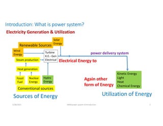
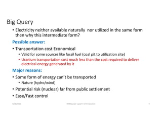
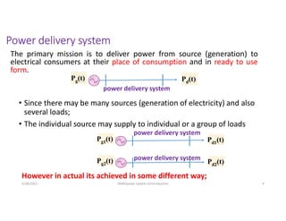
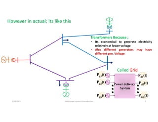
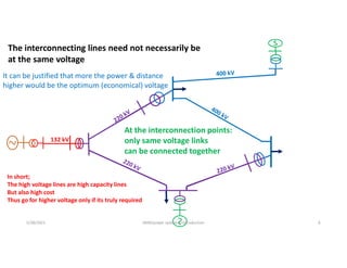
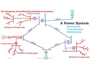
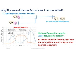
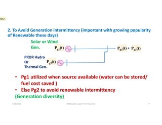

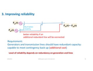
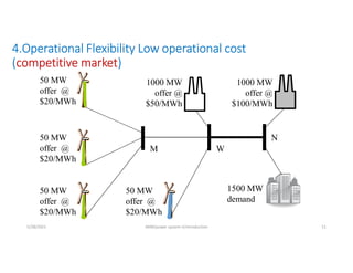
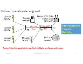
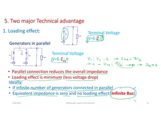
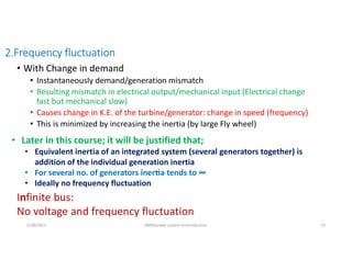
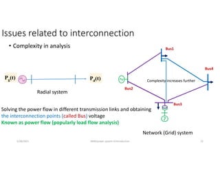
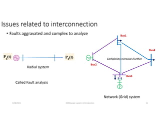


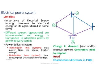
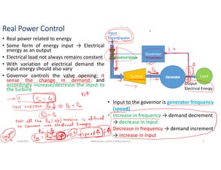
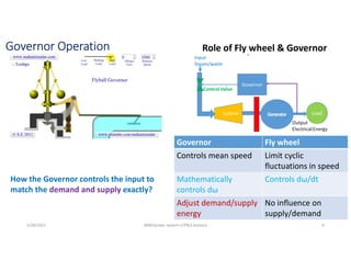
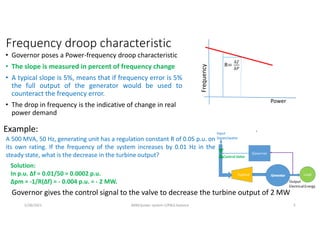
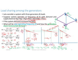
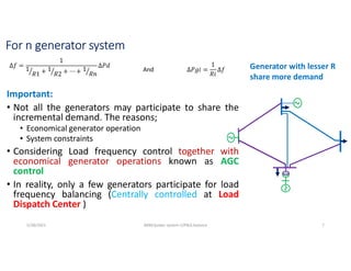


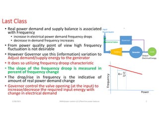
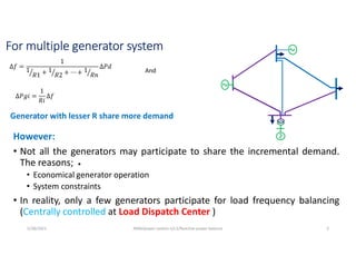
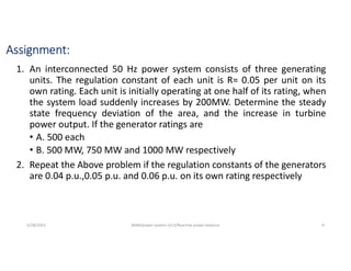
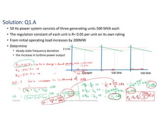
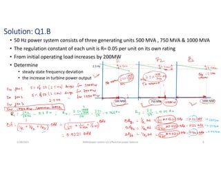
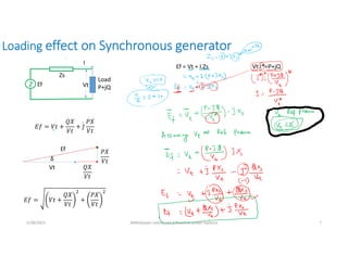
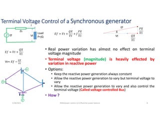
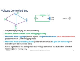
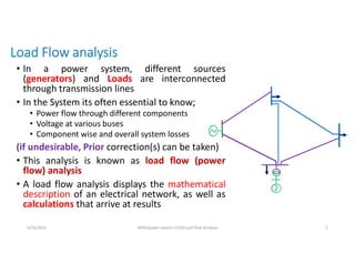

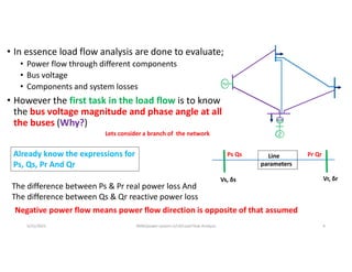
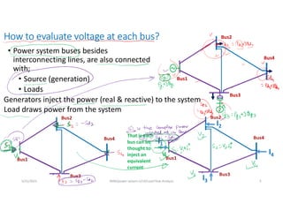
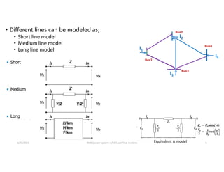
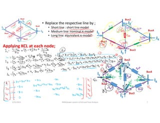
![Some peculiarities of above matrix
• Square matrix of 4 x 4 (For a N bus system N x N)
• Symmetric matrix
• Elements of the matrix are only the physical
parameters (Don’t depends on loading condition)
• Diagonal elements Yii : shunt admittance at the node +
sum of the branches series admittance connected to
the node
• Off diagonal elements Yij : negative of branch series
admittance connected between ith & jth node
In Short;
In short, The Matrix follows a systematic formulation
and no need to derive each time
y23
y20
y40
y10
y30
5/31/2021 AKM/power system-ii/L4/Load Flow Analysis 8
[ IBUS ] = [ Matrix ] [VBUS]
Popularly know as:
Bus admittance matrix
YBUS Matrix](https://image.slidesharecdn.com/akmsirpsa2-250822034814-3fa331e0/85/power-system-electrical-engineering-Note-43-320.jpg)
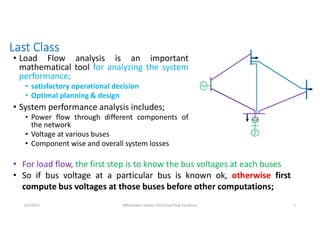
![Characteristics of the Bus admittance (YBUS )matrix;
• Square matrix, of size n x n (For a n bus system)
• Symmetric matrix
• Elements of the matrix are only the physical parameters (r.l,c)
(Don’t depends on loading condition)
6/3/2021 AKM/power system-ii/L5/Load Flow Equations 3
[ IBUS ] = [ YBUS ] [VBUS]
• Correlation between Bus injected current vector and bus voltage vector
Elements of the Ybus Matrix are defined as;
• Diagonal elements Yii : shunt admittance at the node + sum of the branches series admittance
connected to the node
• Off-diagonal elements Yij : negative of branch series admittance connected between ith & jth
node
(That is, for a given network it needs to be computed only once)](https://image.slidesharecdn.com/akmsirpsa2-250822034814-3fa331e0/85/power-system-electrical-engineering-Note-46-320.jpg)
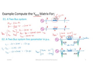
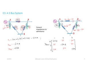
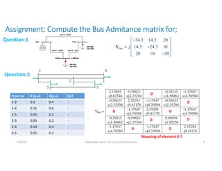
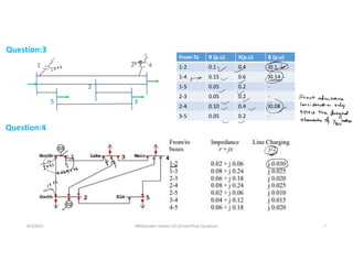
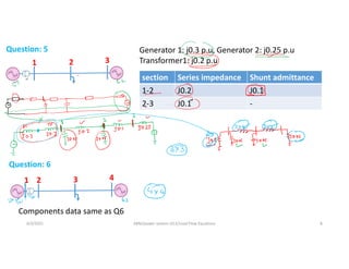
![Application of YBUS Matrix
• For any general system;
• So Bus Voltages can be calculated as;
• ZBUS is called Bus Impedance matrix
• However ZBUS Matrix is rarely computed by inverse of YBUS Matrix
• There are methods to compute ZBUS Matrix directly
• But by whatever methods YBUS or ZBUS Matrixes would be computed, the
above expression can be used to compute Bus voltages only if bus injected
currents are known explicietly
[ IBUS ] = [ YBUS ] [VBUS]
[ VBUS ] = [ YBUS ]-1 [IBUS]
[ VBUS ] = [ ZBUS ] [IBUS]
(because for a practical system YBUS Matrix is a sparse matrix & often its not possible to
compute its inverse)
6/3/2021 AKM/power system-ii/L5/Load Flow Equations 9](https://image.slidesharecdn.com/akmsirpsa2-250822034814-3fa331e0/85/power-system-electrical-engineering-Note-52-320.jpg)
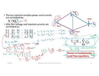
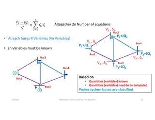
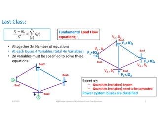
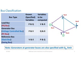
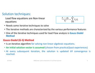
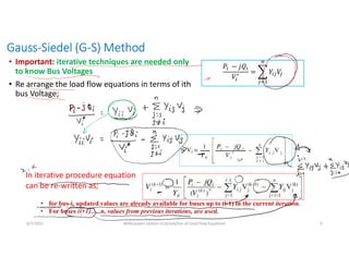
![Algorithm for GS method
Suppose all the buses (except slack bus) are load buses
1. Read physical parameters & specified Bus variables
2. Formulate the bus admittance matrix YBUS
3. Start iteration count k=0; Assume initial voltages for all
buses; [In practical power systems, the magnitude of the bus
voltages is close to 1.0 p.u. Hence, the voltages at all (n-1) buses
(except slack bus) may be assumed to be 1.0+j0]
4. increase iteration count k=k+1
5. For i=2 to n; Update the voltages given by;
Bus2
Bus1
Bus3
Bus4
6. Check convergence criterion If not go back to step 4
7. Compute slack bus power
6/7/2021 AKM/power system-ii/L6/solution of Load Flow Equations 6
With assumption bus 1 is slack bus](https://image.slidesharecdn.com/akmsirpsa2-250822034814-3fa331e0/85/power-system-electrical-engineering-Note-60-320.jpg)
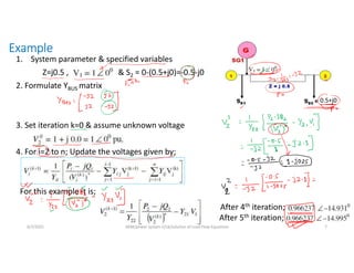
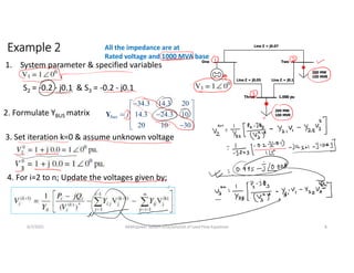
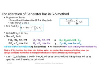
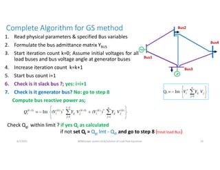
![8. Update the bus voltages as;
10. Check convergence criterion If not k = k+1 & go back to step 4
11. Compute slack bus power Suffix 1: with assumption bus 1 is
slack bus
6/7/2021 AKM/power system-ii/L6/solution of Load Flow Equations 11
Compute bus voltage as;
[Since Voltage magnitude is specified at PV bus]
Go to step 9
9. Increase bus count i=i+1; if I ˂= n go to step 6](https://image.slidesharecdn.com/akmsirpsa2-250822034814-3fa331e0/85/power-system-electrical-engineering-Note-65-320.jpg)
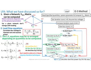
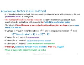
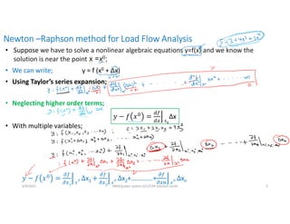
![=
[ Actual f - calculated f ] [ correction]
=[ Jacobean Matrix ]
6/9/2021 AKM/power system-ii/L7/LFA solution contd 6
• For set of nonlinear expressions with multiple variables;
Error vector
correction vector
In Matrix Form;
𝟎 𝝏𝒇
𝝏𝒙𝟏
𝒙
𝟎 x1
𝝏𝒇
𝝏𝒙𝟐
𝒙
𝟎 x2+………….+
𝝏𝒇
𝝏𝒙𝒏 𝒙
𝟎 xn
𝟏 𝟏
𝟎 𝝏𝒇𝟏
𝝏𝒙𝟏
𝒙
𝟎 x1
𝝏𝒇𝟏
𝝏𝒙𝟐
𝒙
𝟎 x2+………….+
𝝏𝒇𝟏
𝝏𝒙𝒏 𝒙
𝟎 xn
𝟐 𝟐
𝟎 𝝏𝒇𝟐
𝝏𝒙𝟏
𝒙
𝟎 x1
𝝏𝒇𝟐
𝝏𝒙𝟐
𝒙
𝟎 x2+………….+
𝝏𝒇𝟐
𝝏𝒙𝒏 𝒙
𝟎 xn
𝒏
𝟎 𝝏𝒇𝒏
𝝏𝒙𝟏
𝒙
𝟎 x1
𝝏𝒇𝒏
𝝏𝒙𝟐
𝒙
𝟎 x2+………….+
𝝏𝒇𝒏
𝝏𝒙𝒏 𝒙
𝟎 xn
Δf=JΔx
Δx=J-1Δf
xk+1=xk+ Δxk](https://image.slidesharecdn.com/akmsirpsa2-250822034814-3fa331e0/85/power-system-electrical-engineering-Note-71-320.jpg)
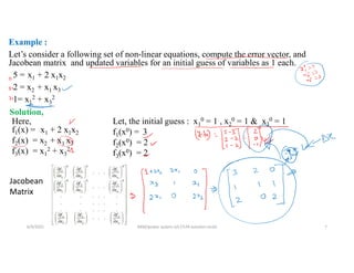


![=
[ Jacobean Matrix ]
6/14/2021 AKM/power system-ii/L8/N-R,LF solution 2
• For set of nonlinear expressions with multiple variables;
Error vector Correction vector
Newton –Raphson iterative method
In short; Δx=J-1Δf x1=x0+ Δx0
Y1= f1 (x1, x2, x3,…. xn)
Y2= f1 (x1, x2, x3,…. xn)
Yn= f1 (x1, x2, x3,…. xn)
For example
5 = x1 + 2 x1x2
2 = x2 + x1 x3
1= x1
2 + x3
2
If 𝟏
𝟎
𝟐
𝟎
𝟑
𝟎
𝒏
𝟎 be the initial assumptions for the variables, and the corrections in
respective variables are Δx1 , Δx2 ,…… Δxn then;
Note: Possible, if J is a square matrix;
means;
number of equations must be
equal to number of variables
In general, xk+1=xk+ Δxk](https://image.slidesharecdn.com/akmsirpsa2-250822034814-3fa331e0/85/power-system-electrical-engineering-Note-75-320.jpg)
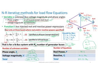
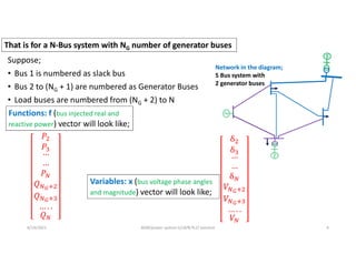
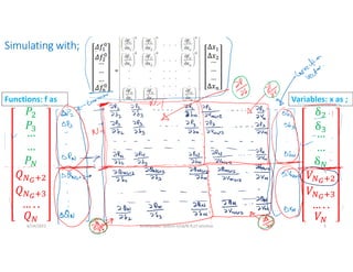
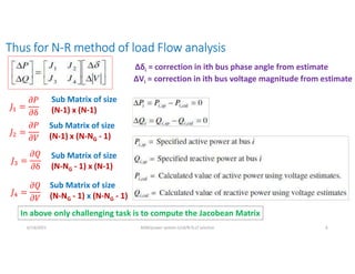
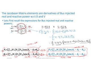
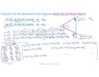
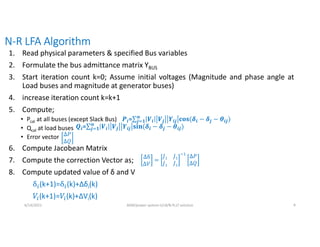

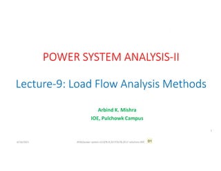

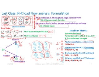
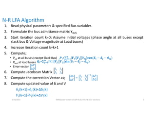
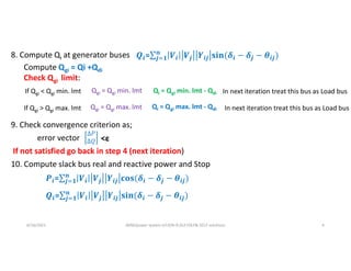
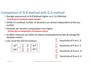
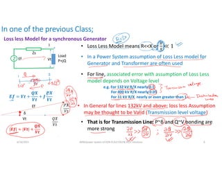
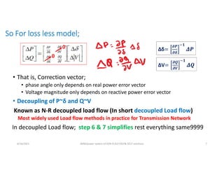
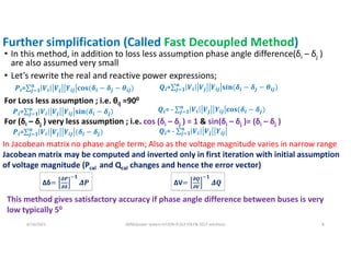
![Approximate Load Flow (called DC Load Flow)
• Additional Assumption: Reactive Power Flow in the Network
assumed zero;
• All the bus voltages magnitude are 1 p.u.
• No need for reactive power consideration
• Need to solve only the phase angle (δ)
• Recall the Bus injected real Power flow expression of Fast Decoupled
Load Flow;
• With all bus voltages to be one;
• Set of Linear simultaneous equation, may be expressed as;
[P]=[B] [δ]
That is [δ]= [B]-1 [P]
• No iteration at all
• Approximate Load flow only
6/16/2021 AKM/power system-ii/L9/N-R,DLF,FDLF& DCLF solutions 9
Vt 𝑄𝑋
𝑉𝑟
𝑃𝑋
𝑉𝑟
Vs
δ
𝑷𝒊=∑ 𝑽𝒊 𝑽𝒋 𝒀𝒊𝒋 (𝜹𝒊 − 𝜹𝒋
𝒏
𝒋 𝟏 )
𝑷𝒊=∑ 𝒀𝒊𝒋 (𝜹𝒊 − 𝜹𝒋
𝒏
𝒋 𝟏 )
Δδ=
𝝏𝑷
𝝏𝜹
𝟏
𝜟𝑷
ΔV=
𝝏𝑸
𝝏𝑽
𝟏
𝜟𝑸](https://image.slidesharecdn.com/akmsirpsa2-250822034814-3fa331e0/85/power-system-electrical-engineering-Note-93-320.jpg)