Unleash the Potential with us and explore cell painting for Phenotypic Profiling in Drug Discovery! We summarised the most important information from the JUMP CP Pilot dataset for you on this poster. Download our poster for free now and share it with your colleagues. Feel free to also have a look at our other posters available for download directly from our website as well: https://www.kmlvision.com/category/posters/ References: 1. Chandrasekaran SN et al. bioRxiv https://doi.org/10.1101/2022.01.05.475090. 2. Bray MA et al. Nat Protoc. 2016 Sep; 11(9): 1757-1774. 3. Omta W et al. Assay Drug Dev Technol. 2016; 14(8): 439-452. 4. KML Vision GmbH, IKOSA (software), 2023, Graz, Austria, software available at https://app.ikosa.ai/ Links: Visit our website: www.kmlvision.com About the company: https://www.kmlvision.com/ KML Vision GmbH, Nikolaiplatz 4, 2nd floor, 8020 Graz, Austria Contact us: slideshare@kmlvision.com

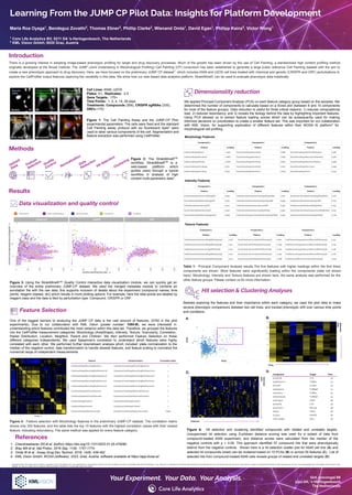
1. Copyright notice: this poster and its content is copyright of Core Life Analytics B.V. Any redistribution or reproduction of part or all of the contents in any form is prohibited other than the following: 1) you may print or download to a local hard disk extracts for your personal and non-commercial use only, and 2) you may copy the content to individual third parties for their personal use, but you must acknowledge Core Life Analytics as the source of the
material. You may not, except with our express written permission, distribute or commercially exploit the content.
Your Experiment. Your Data. Your Analysis. Sint Janssingel 88
5211 DA, ‘s-Hertogenbosch
The Netherlands
There is a growing interest in adopting image-based phenotypic profiling for target and drug discovery processes. Much of the growth has been driven by the use of Cell Painting, a standardized high content profiling method
originally developed at the Broad Institute. The JUMP (Joint Undertaking in Morphological Profiling) Cell Painting (CP) consortium has been established to generate a large public reference Cell Painting dataset with the aim to
create a new phenotypic approach to drug discovery. Here, we have focused on the preliminary JUMP CP dataset1
, which includes A549 and U2OS cell lines treated with chemical and genetic (CRISPR and ORF) perturbations to
explore the CellProfiler output features capturing the variability in this data. We show how our web-based data analytics platform, StratoMineR, can be used to evaluate phenotypic data holistically.
Maria Roa Oyaga1
, Bendeguz Zovathi2
, Thomas Ebner2
, Phillip Clarke2
, Wienand Omta1
, David Egan1
, Philipp Kainz2
, Victor Wong1
Learning From the JUMP CP Pilot Data: Insights for Platform Development
Introduction
Results
References
1. Chandrasekaran SN et al. bioRxiv https://doi.org/10.1101/2022.01.05.475090.
2. Bray MA et al. Nat Protoc. 2016 Sep; 11(9): 1757-1774.
3. Omta W et al. Assay Drug Dev Technol. 2016; 14(8): 439-452.
4. KML Vision GmbH, IKOSA (software), 2023, Graz, Austria, software available at https://app.ikosa.ai/
Methods
Figure 2: The StratoMineRTM
workflow. StratoMineRTM
is a
web-based platform which
guides users through a typical
workflow in analysis of high
content multi-parametric data3
.
Upload
Data Feature
Selection
Quality
Control
Normalization
Data
Reduction
Hit Selection
Clustering
Data visualization and quality control
Figure 3: Using the StratoMineR™ Quality Control interactive data visualization module, we can quickly get an
overview of the entire preliminary JUMP-CP dataset. We used the merged metadata module to combine an
annotation file with the raw data, this supports inclusion of details about the experiment (compound names, time
points, reagent classes, etc) which results in more plotting options. For example, here the data points are labeled by
reagent class and the data is tiled by perturbation type: Compound, CRISPR or ORF.
Figure 1: The Cell Painting Assay and the JUMP-CP Pilot
experimental parameters. The cells were fixed and the standard
Cell Painting assay protocol with six fluorescent dyes2
were
used to label various components of the cell. Segmentation and
feature extraction was performed using CellProfiler.
Cell Lines: A549, U2OS
Plates: 51, Replicates: 2-5
Gene Targets: 175+
Time Points: 1, 2, 4, 14, 28 days
Treatments: Compounds (306), CRISPR sgRNAs (335),
ORFs (175)
Hoechst
33342
Concanavalin
A/Alexa Fluor488
conjugate
SYTO 14 green
fluorescent stain
Phalloidin Alexa
Fluor 568
conjugate
MitoTracker Deep
Red
Dimensionality reduction
Component 1 Component 2 Component 3
Feature Loading Feature Loading Feature Loading
NucleiIntensityMaxIntensityEdgeER 0.950 CellsIntensityMeanIntensityEdgeBrightfield 1.000 NucleiIntensityStdIntensityEdgeBrightfield 0.776
NucleiIntensityStdIntensityEdgeER 0.925 CellsIntensityMeanIntensityEdgeHighZBF 0.999 CellsIntensityMaxIntensityHighZBF 0.753
CellsIntensityMaxIntensityER 0.910 CellsIntensityMeanIntensityLowZBF 0.997 CellsIntensityStdIntensityBrightfield 0.753
NucleiIntensityMaxIntensityER 0.900 CellsIntensityMeanIntensityBrightfield 0.997 NucleiIntensityMassDisplacementBrightfield 0.740
NucleiIntensityStdIntensityEdgeAGP 0.859 CellsIntensityUpperQuartileIntensityBrightfield 0.997 CellsIntensityMaxIntensityBrightfield 0.738
Component 1 Component 2 Component 3
Feature Loading Feature Loading Feature Loading
CellsAreaShapeExtent -0.902 NucleiAreaShapeZernike55 0.886 NucleiAreaShapeMinFeretDiameter 0.982
CellsAreaShapeZernike00 -0.882 NucleiAreaShapeZernike77 0.858 NucleiAreaShapeEquivalentDiameter 0.960
CellsAreaShapeSolidity -0.876 NucleiAreaShapeZernike75 0.840 NucleiAreaShapeMaximumRadius 0.958
CellsAreaShapeZernike95 0.872 NucleiAreaShapeZernike33 0.807 NucleiAreaShapePerimeter 0.948
CellsAreaShapeZernike31 0.845 NucleiAreaShapeZernike71 0.803 NucleiAreaShapeArea 0.945
Intensity Features
Morphology Features
Component 1 Component 2 Component 3
Feature Loading Feature Loading Feature Loading
CellsTextureSumVarianceBrightfield300256 1.028 NucleiTextureCorrelationDNA1003256 -0.801 CellsTextureAngularSecondMomentER1000256 1.022
CellsTextureSumVarianceBrightfield301256 1.021 NucleiTextureInfoMeas1DNA1001256 -0.799 CellsTextureAngularSecondMomentER1001256 1.019
CellsTextureSumVarianceHighZBF301256 1.012 NucleiTextureCorrelationDNA1001256 -0.793 CellsTextureAngularSecondMomentER1002256 1.018
CellsTextureSumVarianceBrightfield302256 1.010 NucleiTextureCorrelationDNA1002256 -0.792 CellsTextureAngularSecondMomentER1003256 1.016
CellsTextureSumVarianceBrightfield500256 1.010 NucleiTextureInfoMeas1DNA1003256 -0.788 CellsTextureDifferenceVarianceER1000256 1.009
Texture Features
Feature Closest Feature Correlation Value
CellsAreaShapeBoundingBoxArea CytoplasmAreaShapeBoundingBoxArea 1
CellsAreaShapeBoundingBoxMaximumX CytoplasmAreaShapeBoundingBoxMaximumX 1
CellsAreaShapeBoundingBoxMaximumY CytoplasmAreaShapeBoundingBoxMaximumY 1
CellsAreaShapeBoundingBoxMinimumY CytoplasmAreaShapeBoundingBoxMinimumY 1
CellsAreaShapeBoundingBoxMinimumX CytoplasmAreaShapeBoundingBoxMinimumX 1
CellsAreaShapeMinFeretDiameter CytoplasmAreaShapeMinFeretDiameter 1
CellsAreaShapeMaxFeretDiameter CytoplasmAreaShapeMaxFeretDiameter 1
CellsAreaShapeCenterY CytoplasmAreaShapeCenterY 1
CellsAreaShapeCenterX CytoplasmAreaShapeCenterX 1
CellsAreaShapeMajorAxisLength CytoplasmAreaShapeMajorAxisLength 0.999
Hit selection & Clustering Analyses
Figure 4: Feature selection with Morphology features in the preliminary JUMP-CP dataset. The correlation matrix
shows only 250 features, and the table lists the top 10 features with the highest correlation values with their closest
feature, indicating redundancy. The same method was applied for every feature category.
Feature Selection
One of the biggest barriers to analyzing the JUMP CP data is the vast amount of features; (5792 in the pilot
experiments). Due to our collaboration with KML Vision (poster number: 1095-B), we were interested in
understanding which features contributed the most variance within this data set. Therefore, we grouped the features
into the CellProfiler measurement categories: Morphology (AreaShape), Intensity, Texture, Granularity, Correlation,
Radial Distribution, Location, Neighbor, Parent and Children. We then performed Feature Selection on these
different categories independently. We used Spearman's correlation to understand which features were highly
correlated with each other. We performed further downstream analysis which included: plate normalization to the
median of the negative control, data transformation to handle skewed features, and feature scaling to normalize the
numerical range of independent measurements
We applied Principal Component Analysis (PCA) on each feature category group based on the samples. We
determined the number of components to calculate based on a Scree plot (between 8 and 10 components
for most of the feature groups). Data reduction is useful for three critical reasons: 1) reduces computational
load, 2) reduces redundancy, and 3) reveals the biology behind the data by highlighting important features.
Using PCA allowed us to extract feature loading scores which can be subsequently used for making
informed decisions on prioritization to create a smaller feature set. This was important for our collaboration
with KML Vision, for supporting exploration of different features within their IKOSA AI platform4
for
morphological cell profiling.
Table 1: Principal Component Analysis results.The five features with higher loadings within the first three
components are shown. More features were significantly loading within the components (data not shown
here). Morphology, Intensity and Texture features are shown here, the same analysis was performed for the
other feature groups. Please contact us for more information.
PCA2
PCA1
Compound Target Time
ponatinib LYN 24
epothilone-b TUBB3 24
briciclib CCND1 24
ixabepilone TUBB4B 24
colchicine TUBB3 24
oxibendazole TUBB4B 24
azeliragon AGER 48
ponatinib LYN 48
puromycin RPL23A 48
GK921 TGM2 48
SU3327 MAPK8 48
LDN-212854 ABL1 48
A.
Figure 6: Hit selection and clustering identified compounds with related and unrelated targets.
Unsupervised hit selection using Euclidean distance scoring was used for a subset of data from
compound-treated A549 experiment, and distance scores were calculated from the median of the
negative controls with p < 0.05. This approach identified 57 compound hits that were phenotypically
distinct from the negative controls. Shown here is a hit selection scatter plot for A549 cell line (A) and
selected hit compounds (inset) can be clustered based on 10 PCAs (B) or across 50 features (C). List of
selected hits from compound-treated A549 cells reveals groups of related and unrelated targets (D).
PCAs
B.
Selected
data
Besides exploring the features and their importance within each category, we used the pilot data to make
several phenotypic comparisons between two cell lines, and tracked phenotypic drift over various time points
and conditions.
1
Core Life Analytics BV, 5211 DA 's-Hertogenbosch, The Netherlands
2
KML Vision GmbH, 8020 Graz, Austria
C.
Selected
data
D.
Features
Compound ORF
CRISPR