Polar orbiting satellites (cf Geostationary) Sun-synchronous daily orbital path
1. 1/34
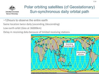
Polar orbiting satellites (cf Geostationary)
Sun-synchronous daily orbital path
~12hours to observe the entire earth
Same location twice daily (ascending /descending)
Low earth orbit (Geo at 36000km)
Delay in receiving data because of limited receiving stations
2. 2/34
Passive and Active instruments for measuring
radiation
Passive Instruments:
– Receive radiation leaving the earth-atmosphere
system
– Measure solar radiation reflected by land &
atmosphere targets (visible light)
– Measure emitted and scattered IR radiation
– Measure microwave radiation emission, scattering
(ice); emission/absorption (liquid water in clouds)
directly related to brightness Temperature
• Active Instruments:
– Send out pulses of radiation, usually at
microwave frequencies
– Measure radiation returned to the sensor
– eg: radars; scatterometers
3. 3/34
Scatterometry Theory:
active sensors measure backscatter
Bragg scattering
Sensors emit microwave energy and measure return signal
Small (2-4cm) capillary waves correspond to wind speed
Bragg scattering: energy at similar wavelengths scattered
https://www.meted.ucar.edu/training_module.php?id=1093#.XElBfteWa71
4. 4/34
Scatterometry
http://manati.orbit.nesdis.noaa.g
ov/datasets/ASCATData.php
ASCAT: on METOP-A, B and C satellites
see:http://manati.orbit.nesdis.noaa.gov/datasets/ASCATData.php/
SCATSAT: more sensitive to heavy rain
replaces OceanSAT similar to old Quickscat
Windsat: Very sensitive to heavy rain and so
only useful in heavy rain-free areas.
AMSR-2: speed only – ok for gale extent
SMAP/SMOS:
SAR: high quality but not yet real-time in easy
view
COMET Training package:
https://www.meted.ucar.edu/EUMETSAT/marine_forecasting/navmenu.php?tab=1&page=2-2-0&type=flash
5. 5/34
Advanced SCATterometer (ASCAT)
Satellite: MetOp-A (2007), B (2012), C (2018)
Channel: 5.25 GHz (5cm); C-Band
coverage: three antennas detecting two swathes 520km
wide separated by ~600km underneath where
insufficient energy comes back.
two passes per day (ascending/descending)
Resolution: 25-50km
TC applications:
Lack of coverage in tropics an issue
Excellent for gale radii and positioning
Excellent for intensity to ~50kn (i.e. weaker systems)
NOAA http://manati.orbit.nesdis.noaa.gov/datasets/ASCATData.php
KNMI http://projects.knmi.nl/scatterometer/tile_prod/tile_app.cgi
NRL: https://www.nrlmry.navy.mil/tc-bin/tc_home2.cgi
7. 7/34
ASCAT positioning: ARCHER
http://tropic.ssec.wisc.edu/real-time/archerOnline/web/index.shtml
Mona 09P: 2151Z 4/1/2019 ASCAT-B
http://tropic.ssec.wisc.edu/real-time/archerOnline/cyclones/2019_09P/web/summaryTable.html
Automatic and usually better than human eye
NRCS: scalar wind display can be the clearest
indication of centre fix in the light wind area
NRCS from NOAA 'manati' web page:
via 'storm' option
eg : Riley Jan2019: NRCS better than Archer
10. 10/34
X
SCATSAT availability
Example: Kelvin (Southern Hemisphere)
Courtesy: KNMI
1. KNMI http://projects.knmi.nl/scatterometer/tile_prod/tile_app.cgi
2. FNMOC: https://www.fnmoc.navy.mil/tcweb/cgi-bin/tc_home.cgi
3. NRL: speed only (irregular coverage currently)
4. Not yet NOAA-coming?
https://manati.star.nesdis.noaa.gov/datasets/ASCATData.php
11. 11/34
X
Exercise: accessing the information
Task: Find ASCAT/SCATSAT for Oma 15P
~18S 162E
Question: Find the latest ASCAT and SCATSAT passes that move over Oma in
the SW Pacific (off New Caledonia)
What time does the pass go over Oma?
What are the highest winds?
Comment on the extent of gales: which quadrant has the furthest extent of
gales?
Use: 1. NOAA https://manati.star.nesdis.noaa.gov/datasets/ASCATData.php
2. KNMI http://projects.knmi.nl/scatterometer/tile_prod/tile_app.cgi
Advanced : 3. Use NOAA 'Storm' option to centre on TC
4. FNMOC: https://www.fnmoc.navy.mil/tcweb/cgi-bin/tc_home.cgi
12. 12/34
X
Radiometers (passive)
Windsat
Examples:1 Ashobaa Courtesy: NOAA
https://manati.star.nesdis.noaa.gov/windsat_images/windsat_storm/storm_id_image_new/2015/windsat15061001_01_ASHOBAA_as.png
2. Kenanga courtesy NRL
https://www.nrlmry.navy.mil/tcdat/tc19/SHEM/06S.KENANGA/ssmi/scat/scat_over_color37/20181221.0037.windsat.WINDSAT_6GHz_color37.
wind.06SKENANGA.3772_090pc_80kts-976mb_162S_804E_sft201812210000_bgt201812210035_bgn201812210000.jpg
https://manati.star.nesdis.noaa.gov/datasets/WindSATData.php
Satellites: Coriolis (2003 extended lifetime! First)
Channel: 6.8-37 GHz
coverage: 1000km wide (>ASCAT, <SCATSAT)
two passes per day(ascending/descending)
Resolution: ~25km
TC applications:
Overestimates winds in rain, but solution to
overcome speed in rainfall being worked on
Not useful for intensity
Sometimes for gale radii outside rain areas
NOAA: https://manati.star.nesdis.noaa.gov/datasets/WindSATData.php
NRL: https://www.nrlmry.navy.mil/tc-bin/tc_home2.cgi
13. 13/34
X
AMSR2 radiometer (passive)
Satellite: GCOM (2012)
Channel: 10.7-36.5GHz
Coverage: 1450km (wider than ASCAT)
Two passes per day
TC applications:
Can be ok for extent of gales
Speed only
Availability same as Windsat
NOAA and NRL
Solution to overcome speed in rainfall
being worked on
ALSO SSMIS radiometer as well
Examples: 1. Dahlia Courtesy: NOAA
https://manati.star.nesdis.noaa.gov/gcom_images/arch/wdsp/GC2017335/zooms/WMBds57.png
2. Kenanga 2018 NRL
https://manati.star.nesdis.noaa.gov/datasets//GCOM2Data.php
14. 14/34
Latest Geostationary:
Himawari-9: 10min; rapidscan 2.5min for target*;
GOES-R: 10-15min; rapidscan 1-5min;
FY-4: 15min rapidscan 2.5min;
KOMPSAT-2A 10min rapidscan 2.0min east Asia
Meteosat: 10min rapidscan 2.5min Europe
Rapidscan best for surface winds
Requires low level cloud exposed so not for central
cloudy regions near TC;
Useful for environmental flow and gale extent.
CIMSS: Surface Adjusted Vis/SWIR Winds
Geostationary satellites
AMV (Cloud drift winds) derived to surface
Rapid scan mode
Acknowledgement: Bessho et al 2018 (IWTC-9)
https://www.wmo.int/pages/prog/arep/wwrp/tmr/documents/T5.2_ppt.pdf
15. 15/34
L-Band Radiometers:
SMAP (Soil Moisture Active Passive)
SMOS (Soil Moisture and Ocean Salinity)
http://www.remss.com/missions/smap/winds/
SMAP coverage image courtesy Meissner et al.2018
microwave ocean emissivity (sea foam) correlates to wind speed
mostly linear at high winds, no reduced sensitivity.
at L-band (21 cm) atmosphere is almost transparent so very small
impacts of rain compared to C, X and Ku bands
L-Band 1.4GHz cf ASCAT C-Band 5.3GHz & SCATSAT Ku-band 13.5GHz
So can resolve high wind speeds
Satellite: SMOS (NASA 2009); SMAP (ESA 2012)
Coverage swathe 1000km SMAP; 1500km SMOS
Resolution 40km (winds averaged over footprint)
TC applications:
Intensity as resolves high wind speeds
40km resolution constraint for small RMW
Good for gale/storm/hurricane radii
Access for real-time an issue (SMOS N/A)
19. 19/34
SMAP availability: NRL
https://www.nrlmry.navy.mil/tc-bin/tc_home2.cgi
NRL: but currently not getting all the images (none for Riley 11S)
https://journals.ametsoc.org/doi/pdf/10.1175/BAMS-D-15-00291.1
Example: Kenanga 2018 75kn
Courtesy: NRL https://www.nrlmry.navy.mil/tcdat/tc19/SHEM/06S.KENANGA/smap/wind/20181221.0100.smap.x.wind.06SKENANGA.80kts-976mb-163S-804E.054pc.jpg
20. 20/34
X
Exercise: accessing the information
Task: Find SMAP for Oma 15P
Question: Find the latest SMAP pass that moves over Oma in the SW Pacific
Note: will have to change date to 18 Feb
What time does the pass go over Oma?
What are the highest winds?
Comment on the extent of gales: which quadrant has the furthest extent of
gales?
How does this compare with ASCAT and SCATSAT from previous exercise?
Use: 1. NOAA https://manati.star.nesdis.noaa.gov/datasets/ASCATData.php
21. 21/34
Microwave Imagery Interpretation
Why Microwave?
Satellites and access
Features of 37 and 85 frequencies
How to use both
Intensity
Acknowledgements: Roger Edson
COMET microwave training
www.meted.ucar.edu
22. 22/34
The Satellites Sensors
• Polar Orbiting Conical Scanner
SSMI, SSMIS, GMI, AMSR2, Windsat
(37GHz)
+ more? TMI (TRMM),
• narrow scan widths but maintains
footprint resolution across the entire scan
• 85GHz higher res than 37GHz
• Cross track AMSU (85GHz only)
• wider scan swaths but resolution
degrades toward the edge of scan
Passive sensing up–radiation from ocean/clouds in 19-24, 37, 85-91GHz ranges
23. 23/34
37-85 GHz differences
85GHz from ocean is absorbed & scattered
by water droplets and further scattered by
large water droplets and hail higher up in
deep convection leading to low brightness
temperatures.
37GHz from ocean is absorbed by cloud/
rain droplets – the radiated energy is
NOT affected by large water droplets and
hail higher up in deep convection leading
to high brightness temperatures.
24. 24/34
37 Vs 85 GHz – summary
• 37 GHz shows region of low-level clouds/rain and so clearly shows low-level
circulation but doesn’t distinguish deep convection from rain.
• 85-91GHz better shows deep convection but can not always see low-level
circulation.
Use colour enhancement to resolve ambiguity between deep convection and
clear ocean surface
25. 25/34
Why is microwave useful?
Microwave allows us to see through the high cloud and resolve
details of the structure and low level circulation
37GHz
low down
85-91GHz
Deep
convection
higher up
IR overnight TC Errol
Where is it?
Is it developing?
26. 26/34
Availability: NRL web pages
http://www.nrlmry.navy.mil/TC.html
Alternate Page at FNMOC www.fnmoc.navy.mil/tcweb/cgi-bin/tc_home.cgi
BoM Image viewer (web)
Advantages
navigation to get lat/lon;
distance to point;
ease of viewing - fast;
local archive.
33. 33/34
37 Vs 85 GHz – Eye size & Parallax
Parallax error:
37 GHz - 5 km or less
85-91 GHz - 10-20 km
Correction back towards satellite
motion is parallel to edge; use 85 windscreen
wiper effect to determine direction
34. 34/34
cold temperatures of deep convection in red against a warmer ocean
background (and land) in blue.
Cold
(Red)
Warm
(Blue)
85 GHz
35. 35/34
warm temperatures of low cloud (and land) in red against a colder ocean background in
blue.
Cold
(Blue)
Warm
(Red)
37 GHz
37. 37/34
85-91GHz Summary
At 85 GHz, energy emitted from the ocean surface is rapidly depleted in
lower to middle portions of convective clouds due to scattering by water
drops and large ice particles
Advantages:
Can penetrate cirrus and reveal internal storm structure such as eyes and convective
bands;
Distinguishes deep convection from lightly raining cloud features;
Offers higher spatial resolution than at 37GHz;
Limitations:
Can not always see low-level circulation;
Cold ocean may look like deep convection – needs colour enhancement to resolve
ambiguity ocean and cloud;
Parallax errors when viewing deep convection (10-20km);
Not available on Windsat;
38. 38/34
37GHz Summary
At 37 GHz, abundant energy emitted by water droplets lower in the
convective cloud is largely unaffected by ice particles higher in the cloud
Advantages:
Can penetrate cirrus and reveal detail within the storm core missed by 85GHz such
as eyes;
Shows regions of low level clouds/rain;
Small parallax error compared to 85GHz;
Limitations:
As deep convection not distinguished well from low clouds then inner core may be
poorly defined;
Lower spatial resolution than on 85GHz;
Some scattering in very intense convection resulting in false signal
– needs colour enhancement to resolve this detail;
Not available on AMSU-B;
39. 39/34
Summary
• There are different techniques used to find the centre: use all available
and the best;
• Microwave images:
– 37GHz low level – generally best for positioning
– 85-91GHz highlights convection in mid-levels
– Use 'color' composite views to help distinguish ocean/low cloud from
higher cloud.
Q Microwave is most useful for determining the centre when …
Q Microwave is least useful for determining the centre when …
40. 40/34
X
Exercises: Gita Feb 2018 09P
Where would you put the centre?
What imagers were most useful?
What other information would help?
Determine position and uncertainty at:
a. 1216UTC on 12/02/2018 __________________________
b. 18UTC on 11/02/2018 __________________________
c. 0304UTC on 10/02/2018 __________________________
d. 1426UTC on 09/02/2018 __________________________
e. 1240UTC on 08/02/2018 __________________________
41. 41/34
X
Exercises: Gita Feb 2018 09P
Where would you put the centre?
ASCAT
https://manati.star.nesdis.noaa.gov/datasets/ASCATData.php:
a. 0852UTC on 12/02/2018 __________________________
b. 2024UTC on 11/02/2018 __________________________
c. 2044UTC on 10/02/2018 __________________________
d. 2104UTC on 09/02/2018 __________________________
e. 2124UTC on 08/02/2018 __________________________
42. 42/34
X
Scatterometry exercise: Gita
a. 12/0852 UTC
https://manati.star.nesdis.noaa.gov/ascat_images/ascat_storm/byu_sh_image/2018/GITA/58726_GITA_180212_0600.avewr.gif
43. 43/34
X
Scatterometry exercise: Gita
b. 2024UTC on 11/02/2018
https://manati.star.nesdis.noaa.gov/ascat_images/ascat_storm/byu_sh_image/2018/GITA/58719_GITA_180212_1200.avewr.gif
https://manati.star.nesdis.noaa.gov/ascat_images/ascat_storm/ascat_25km/storm_sh_image/2018/ascat2518021202_09_GITA_ds.png
44. 44/34
X
Scatterometry exercise: Gita
c. 2044UTC on 10/02/2018
https://manati.star.nesdis.noaa.gov/ascat_images/ascat_storm/ascat_25km/storm_sh_image/2018/ascat2518021000_09_GITA_ds.png
https://manati.star.nesdis.noaa.gov/ascat_images/ascat_storm/ascat_25km/storm_sh_image/2018/ascat2518021101_09_GITA_ds.png
45. 45/34
X
Scatterometry exercise: Gita
d. 09/2103 UTC
https://manati.star.nesdis.noaa.gov/ascat_images/ascat_storm/ascat_25km/storm_sh_image/2018/ascat2518021000_09_GITA_ds.png
https://manati.star.nesdis.noaa.gov/ascat_images/ascat_storm/byu_sh_image/2018/GITA/58719_GITA_180212_1200.avewr.gif
46. 46/34
X
Scatterometry exercise: Gita
e. 2124UTC on 08/02/2018
https://manati.star.nesdis.noaa.gov/ascat_images/ascat_storm/ascat_25km/storm_sh_image/2018/ascat2518021000_09_GITA_ds.png
11/02/18 2024
https://manati.star.nesdis.noaa.gov/ascat_images/ascat_storm/byu_sh_image/2018/GITA/58719_G
ITA_180212_1200.avewr.gif