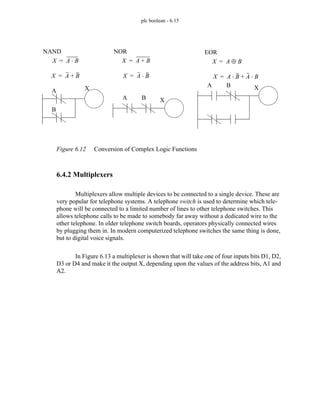
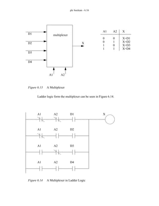
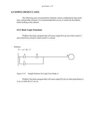
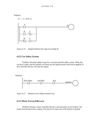
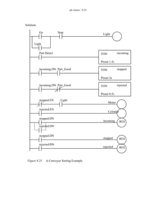
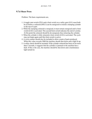
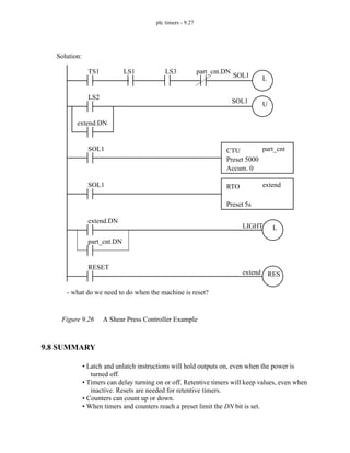
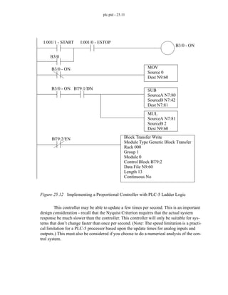
This document provides an overview and introduction to programming programmable logic controllers (PLCs) using ladder logic. It discusses the basic components of ladder logic including rungs, contacts, and coils. It also describes how to connect inputs and outputs, and provides a simple case study example of a ladder logic program.

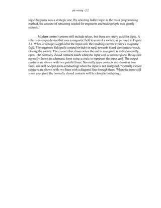
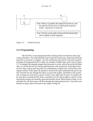
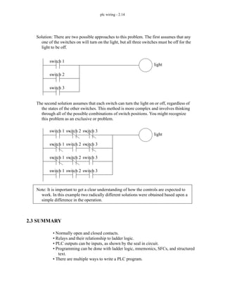

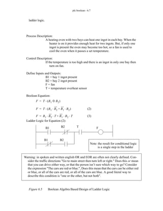
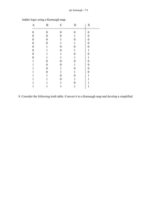
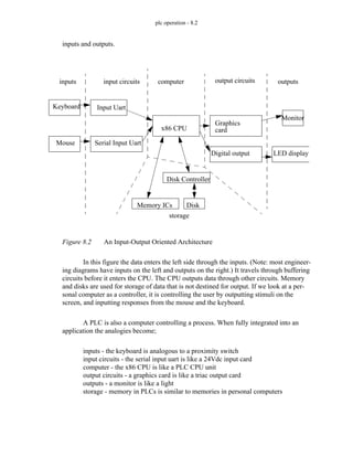
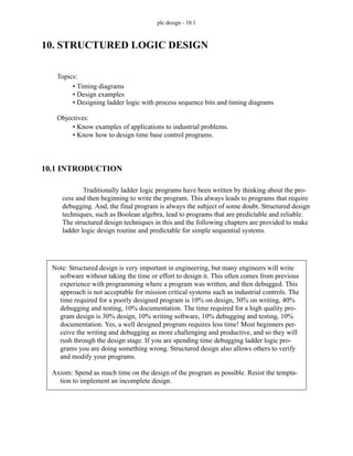
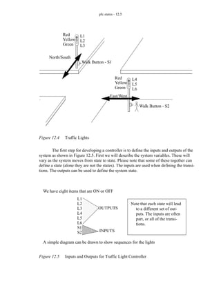
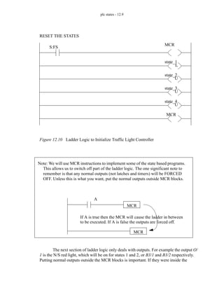
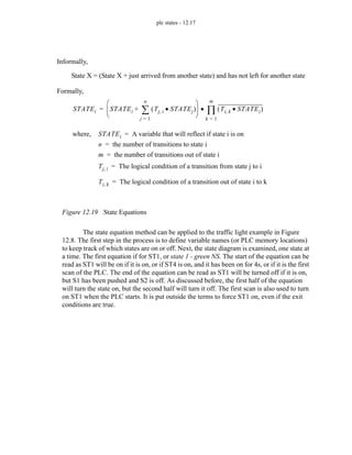
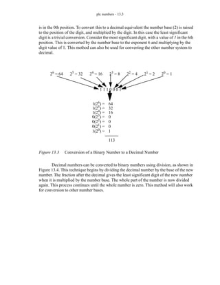
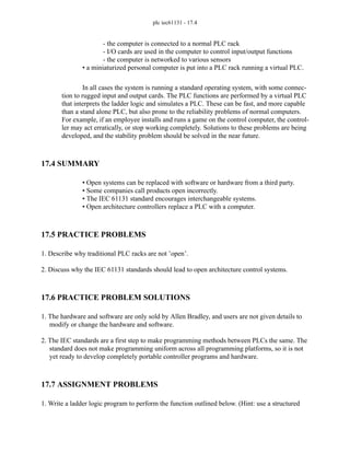
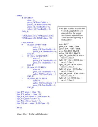
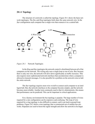
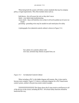
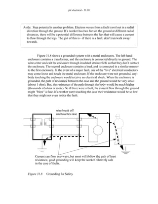
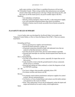
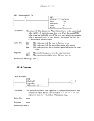
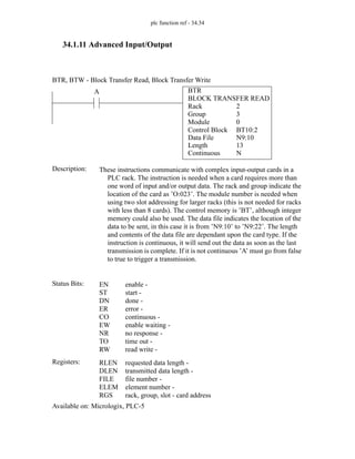
![discrete sensors - 4.19
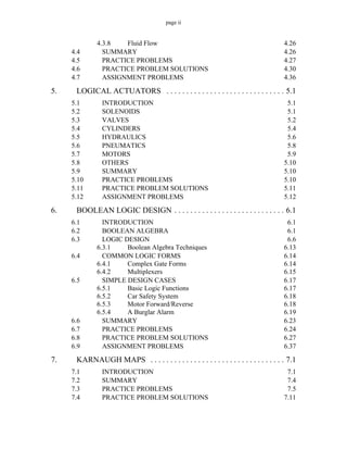
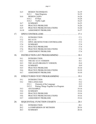
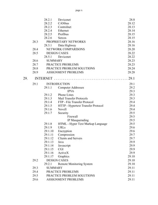
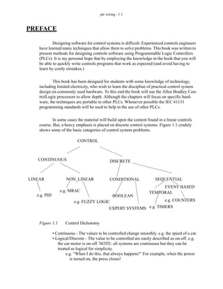
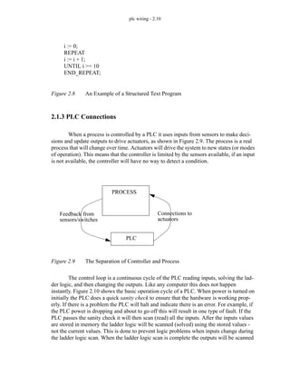
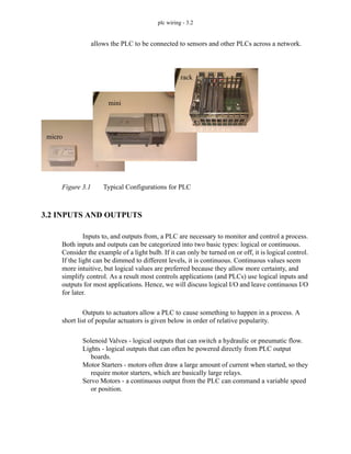
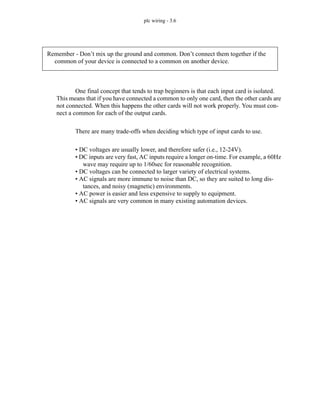
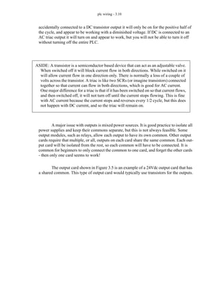
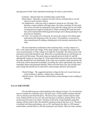
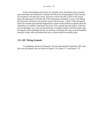
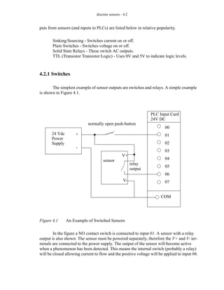
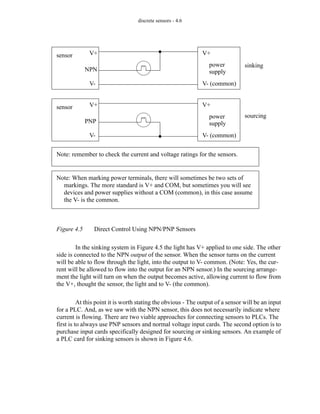
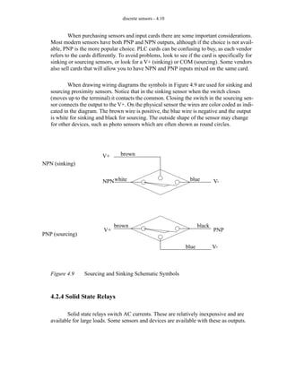
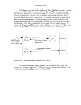
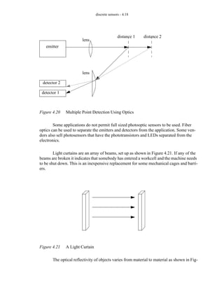
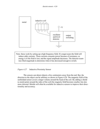
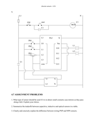
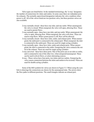
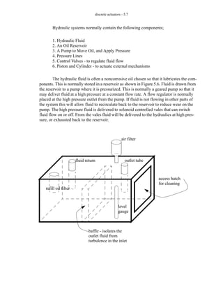
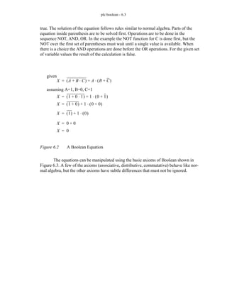
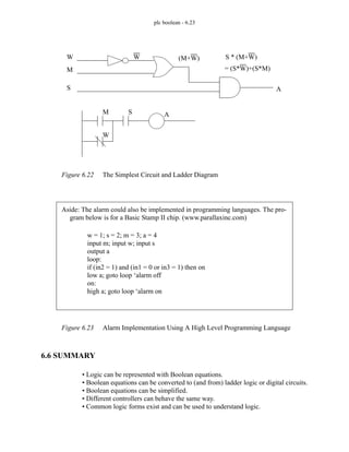
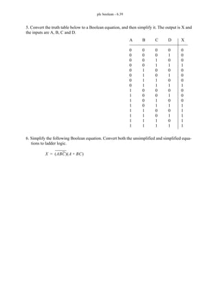
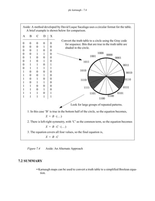
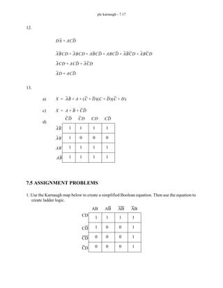
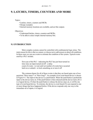
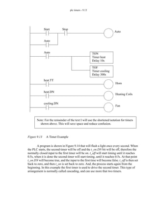
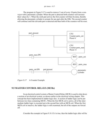
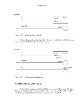
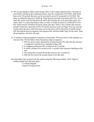
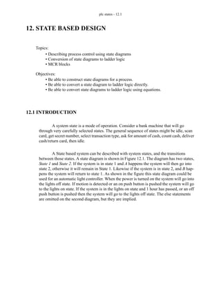
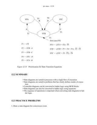
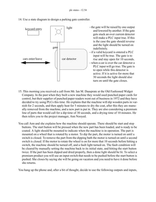
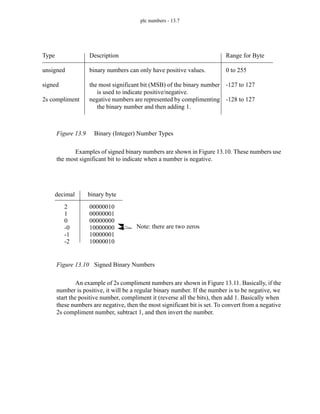
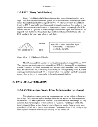
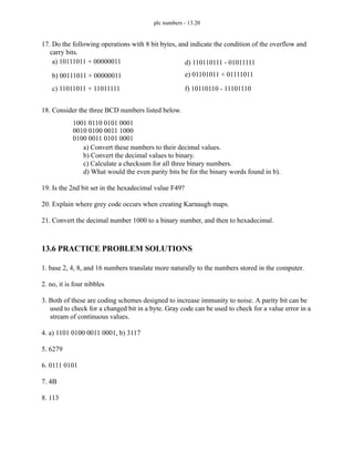
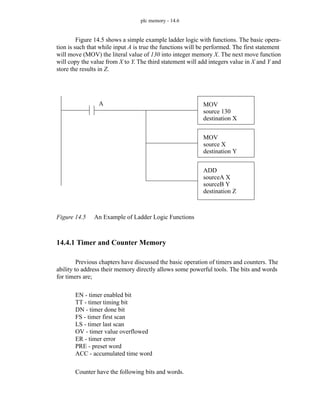
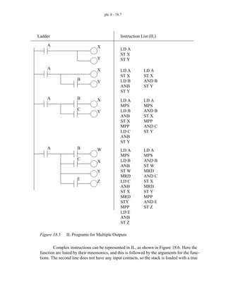
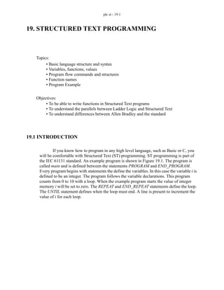
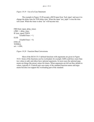
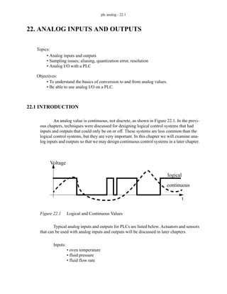
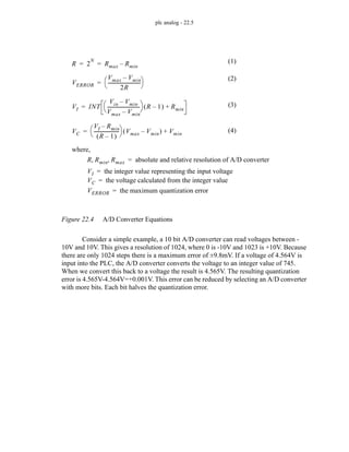
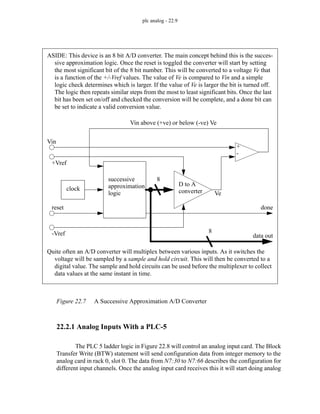
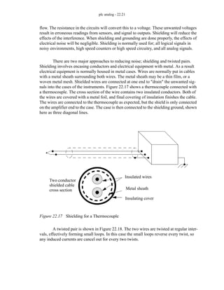
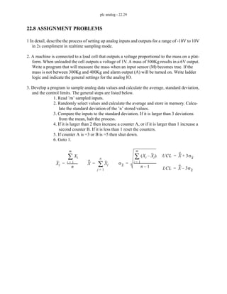
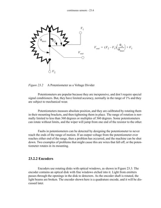
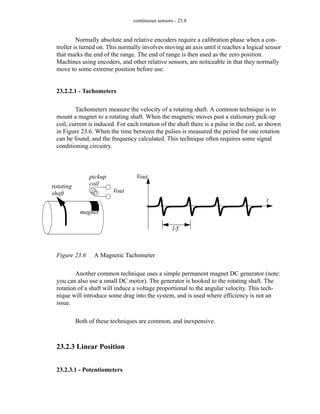
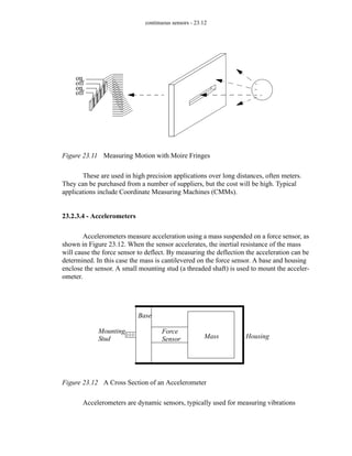
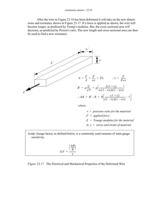
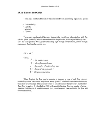
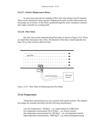
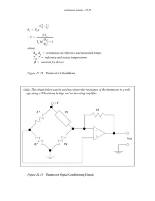
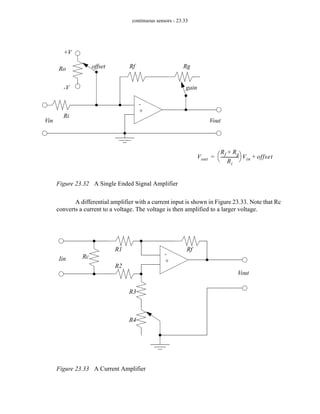
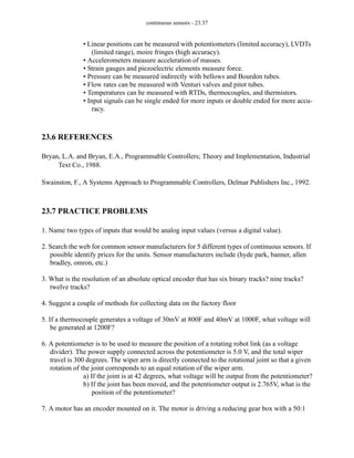
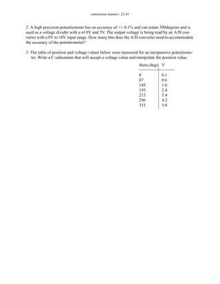
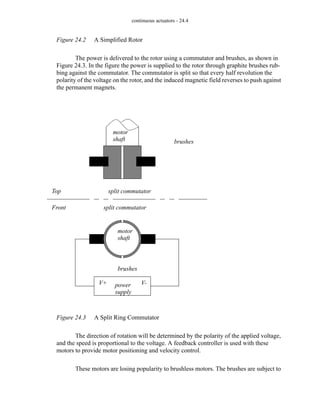
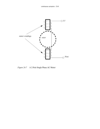
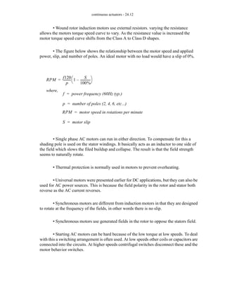
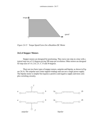
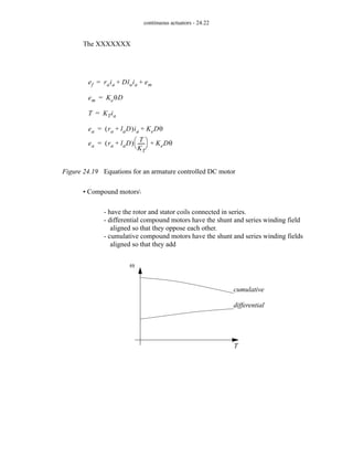
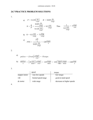
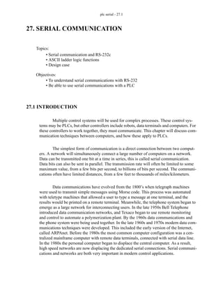
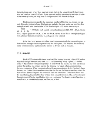
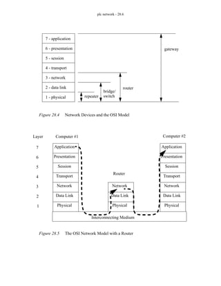
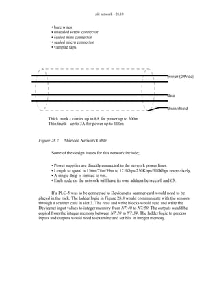
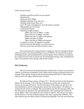
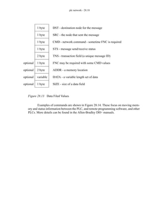
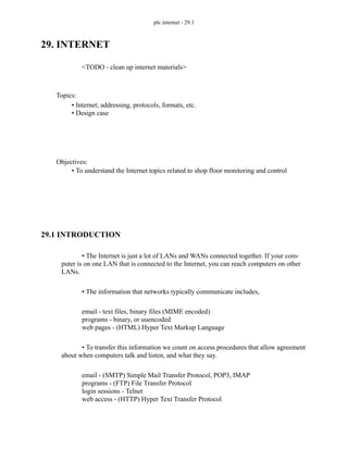
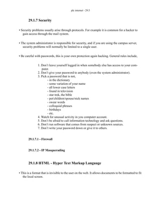
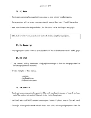
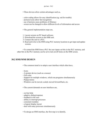
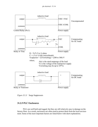
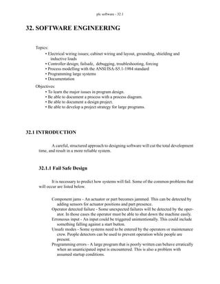
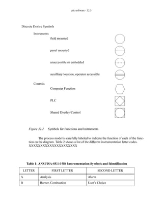
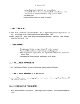
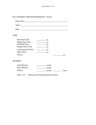
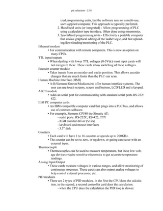
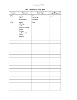
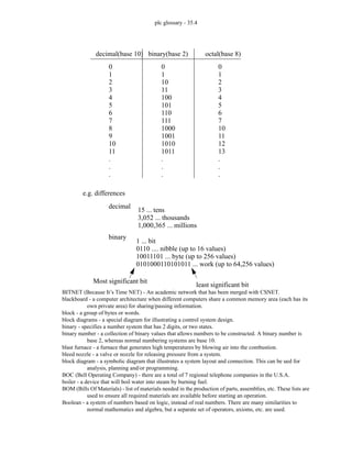
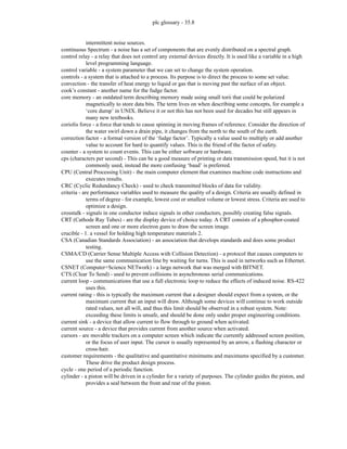
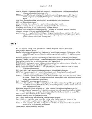
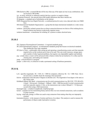
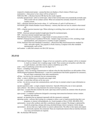
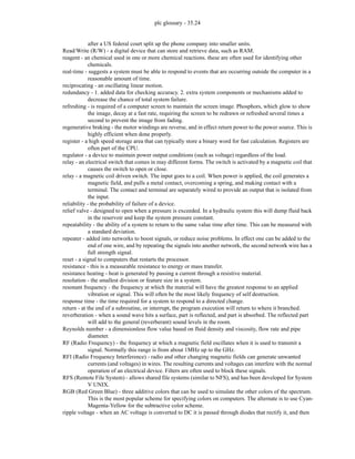
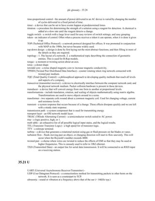
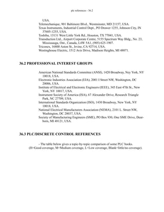
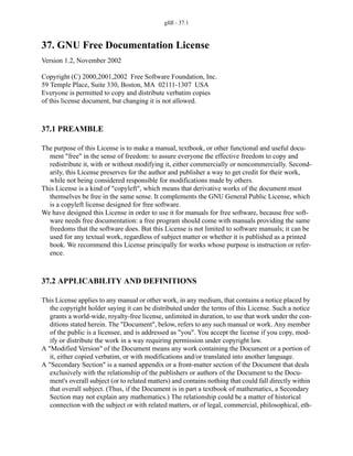
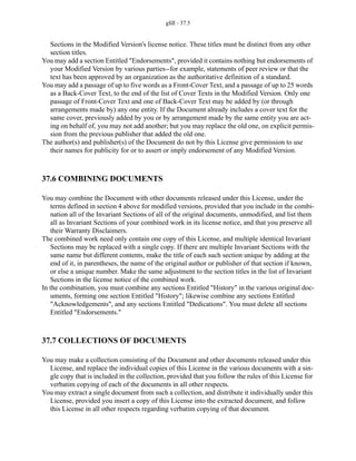
ure 4.22. These values show the percentage of incident light on a surface that is reflected.
These values can be used for relative comparisons of materials and estimating changes in
sensitivity settings for sensors.
Figure 4.22 Table of Reflectivity Values for Different Materials [Banner Handbook of
Photoelectric Sensing]
4.3.4 Capacitive Sensors
Capacitive sensors are able to detect most materials at distances up to a few centi-
meters. Recall the basic relationship for capacitance.
Kodak white test card
white paper
kraft paper, cardboard
lumber (pine, dry, clean)
rough wood pallet
beer foam
opaque black nylon
black neoprene
black rubber tire wall
clear plastic bottle
translucent brown plastic bottle
opaque white plastic
unfinished aluminum
straightened aluminum
unfinished black anodized aluminum
stainless steel microfinished
stainless steel brushed
Reflectivity
90%
80%
70%
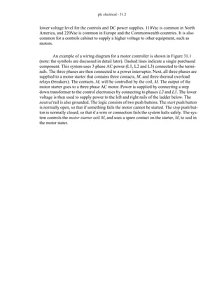
75%
20%
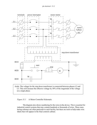
70%
14%
4%
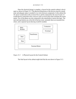
1.5%
40%
60%
87%
140%
105%
115%
400%
120%
nonshiny materials
shiny/transparent materials
Note: For shiny and transparent materials the reflectivity can be higher
than 100% because of the return of ambient light.](https://image.slidesharecdn.com/plc-programmable-logic-controller-book-230318130132-22ebd54b/85/PLC-Programmable-Logic-Controller-Book-pdf-83-320.jpg)
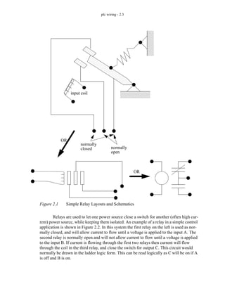
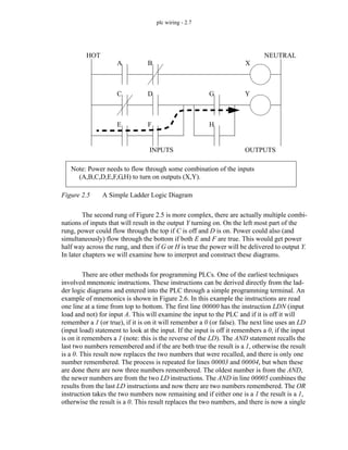
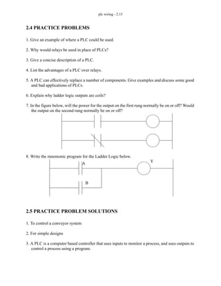
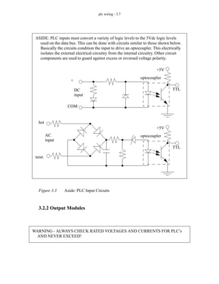
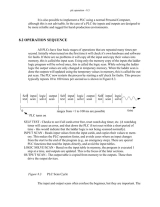
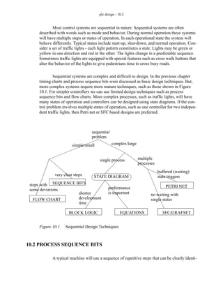
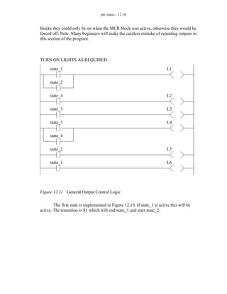
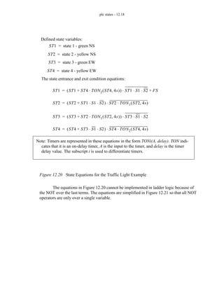
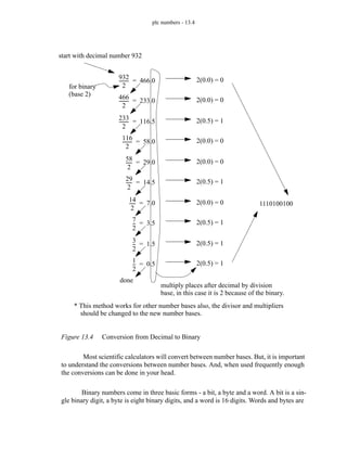
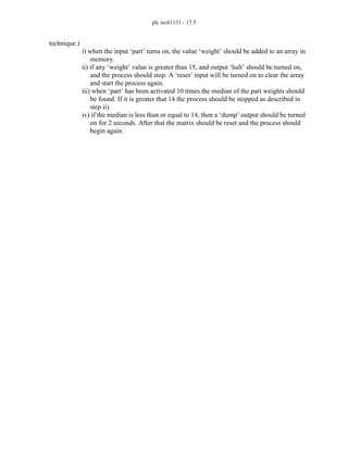
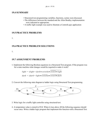
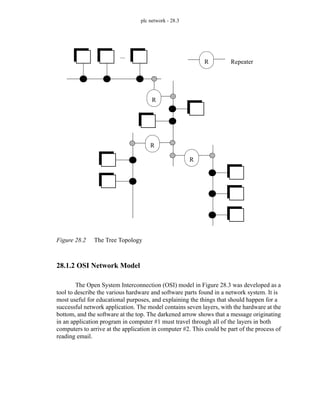
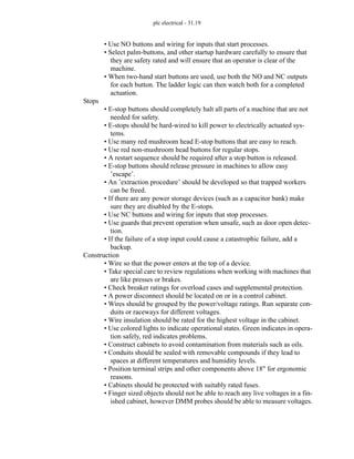
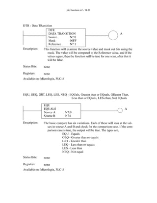
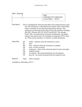
![discrete sensors - 4.23
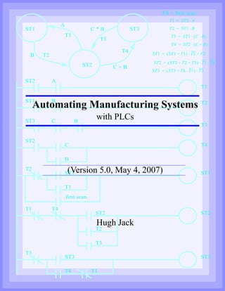
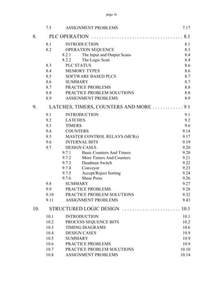
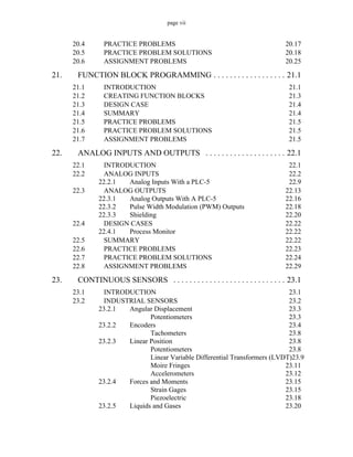
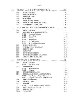
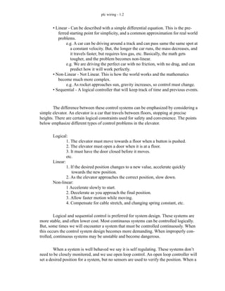
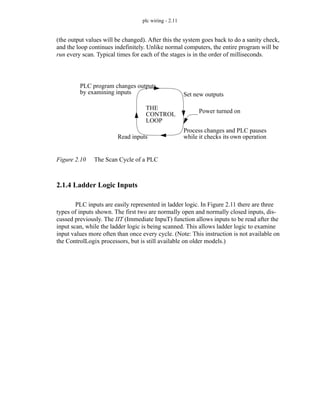
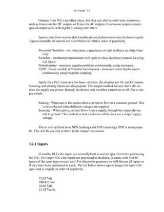
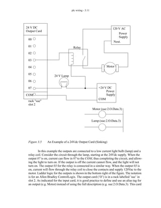
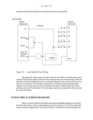
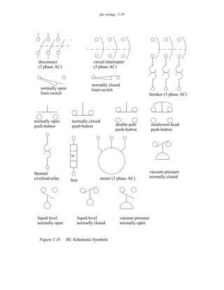
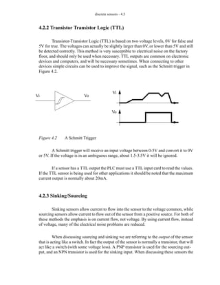
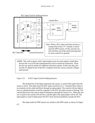
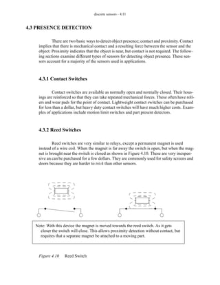
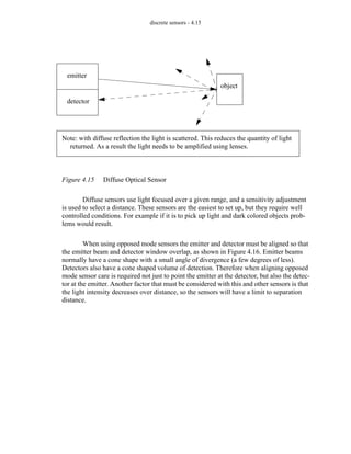
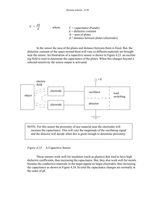
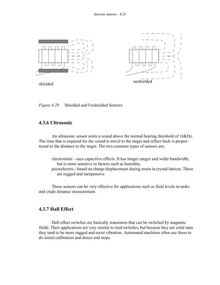
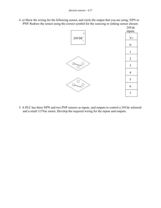
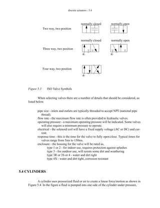
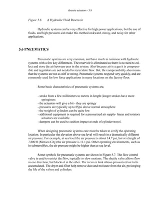
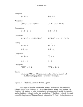
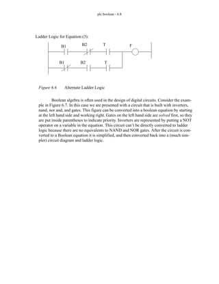
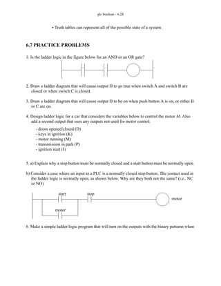
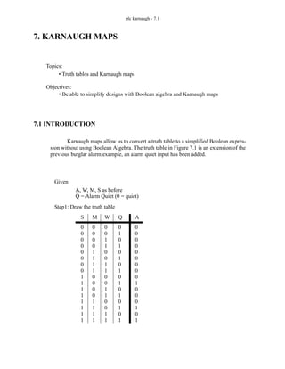
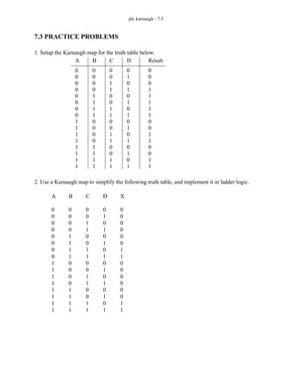
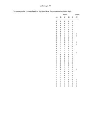
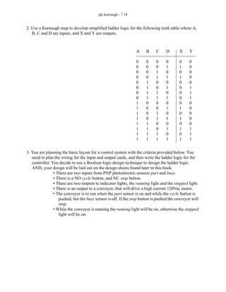
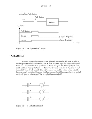
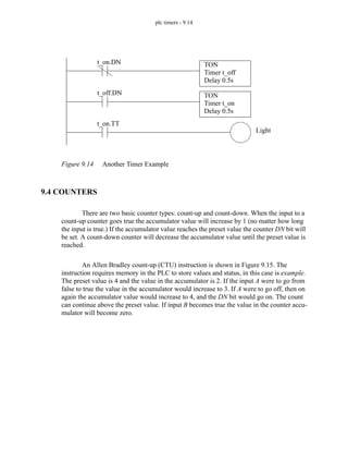
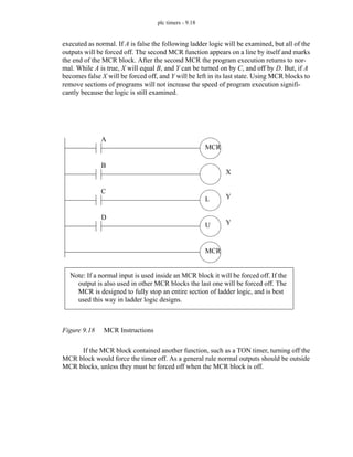
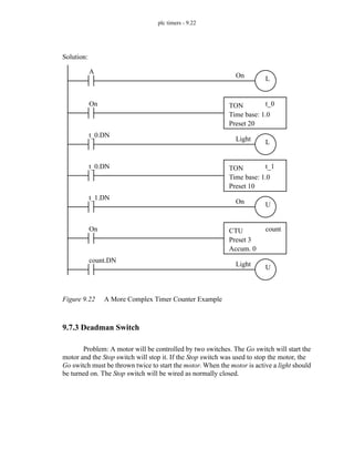
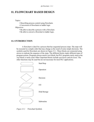
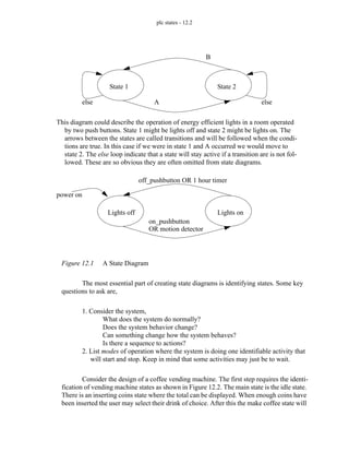
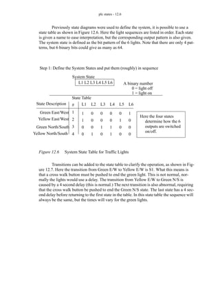
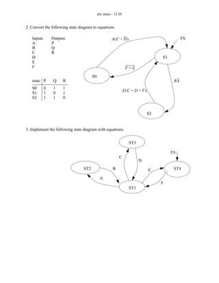
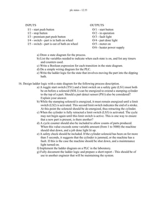
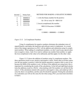
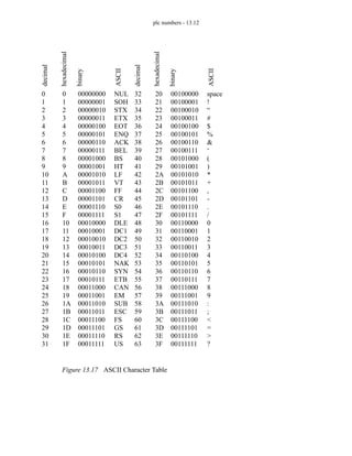
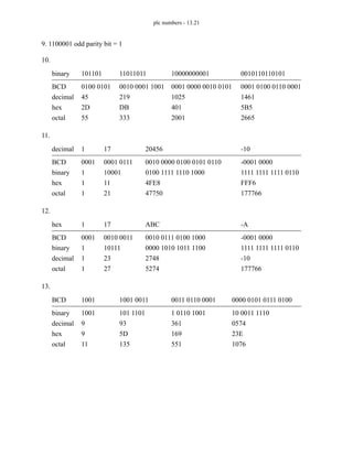
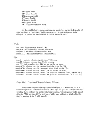
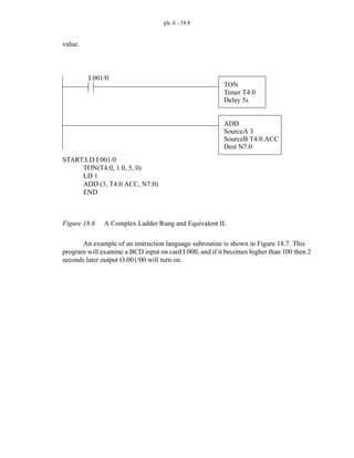
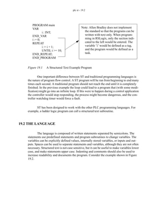
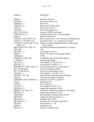
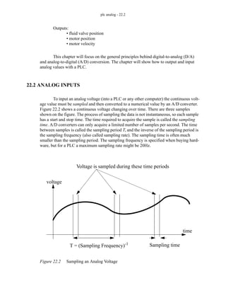
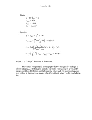
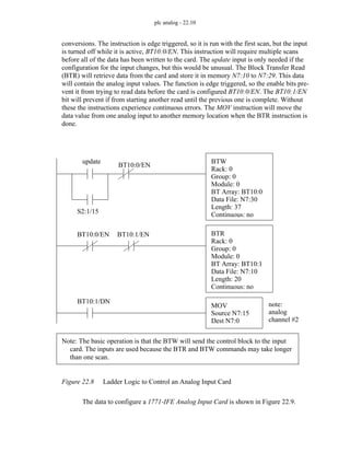
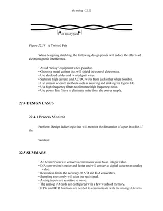
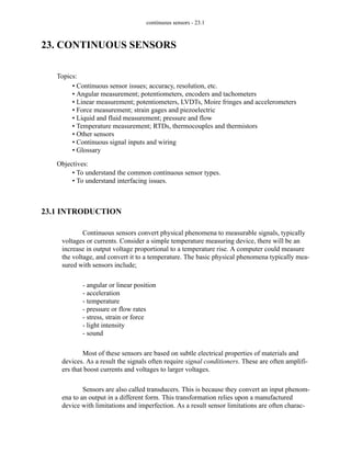
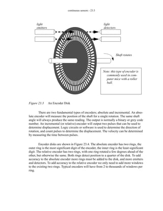
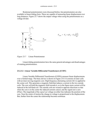
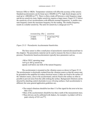
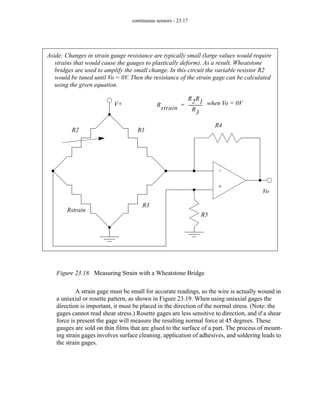
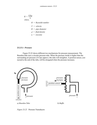
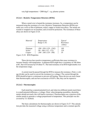
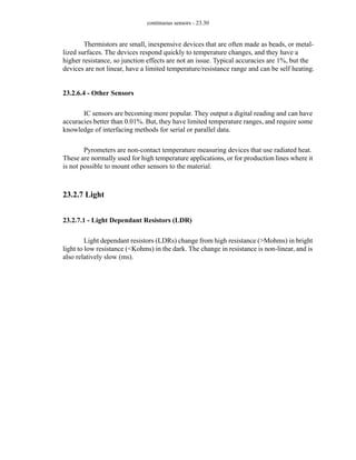
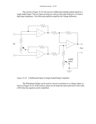
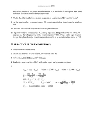
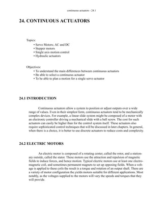
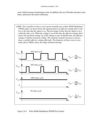
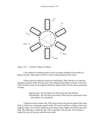
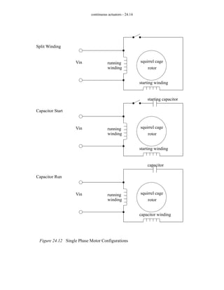
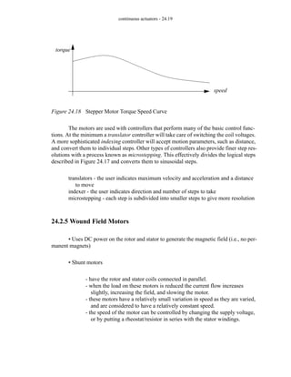
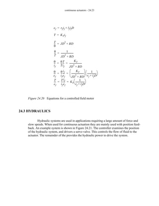
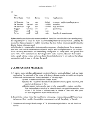
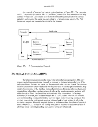
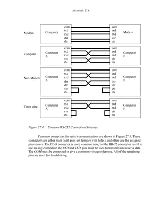
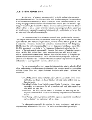
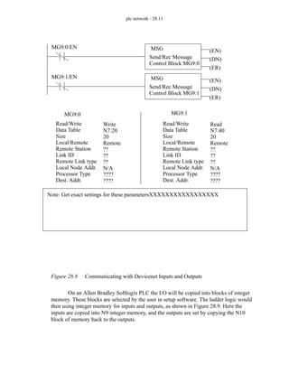
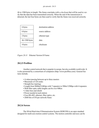
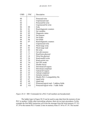
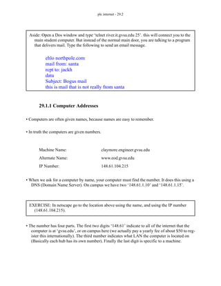
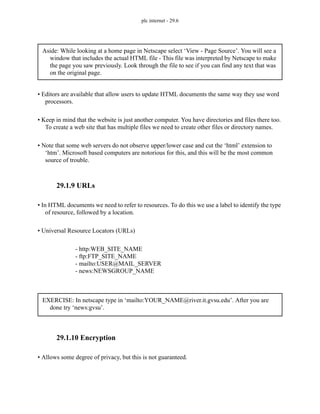
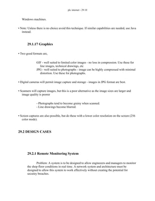
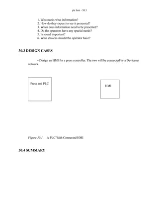
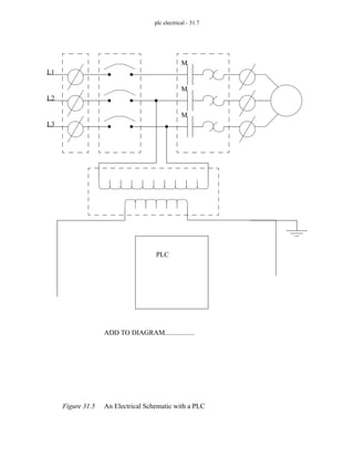
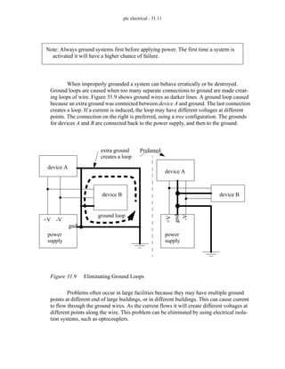
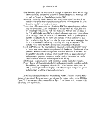
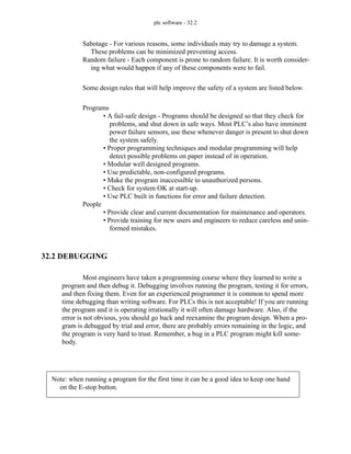
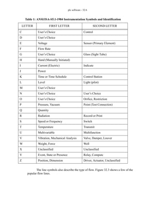
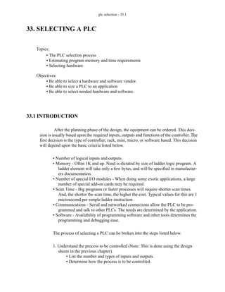
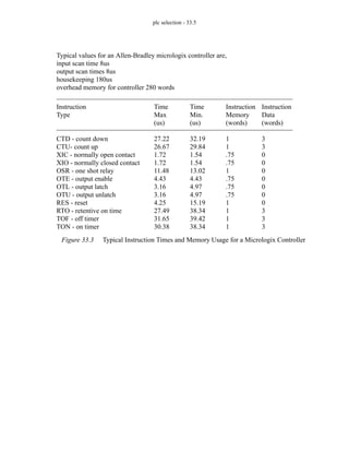
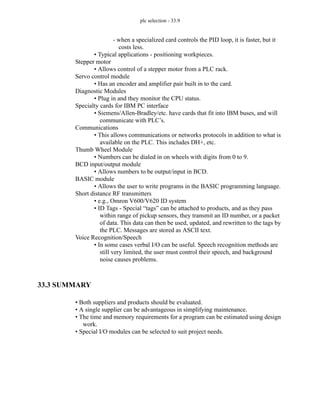
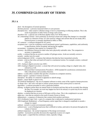
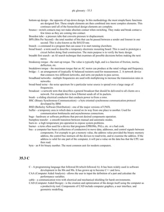
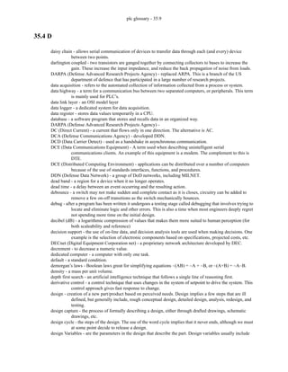
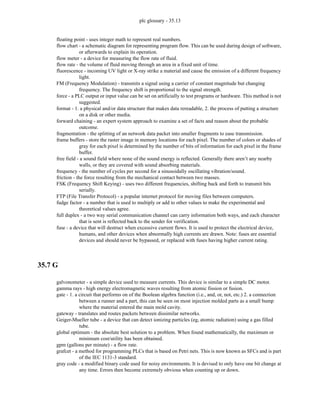
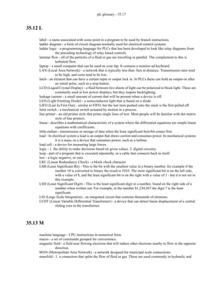
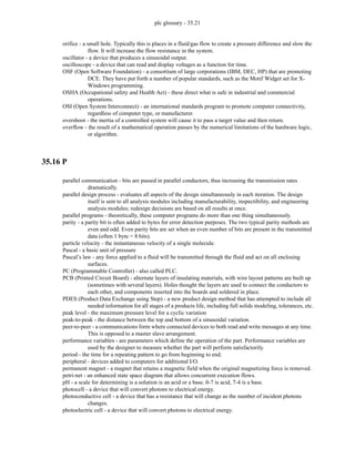
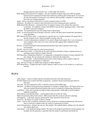
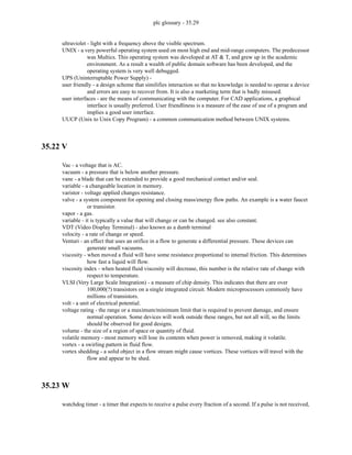
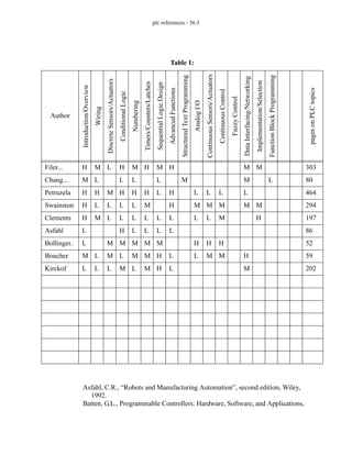
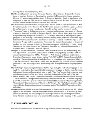
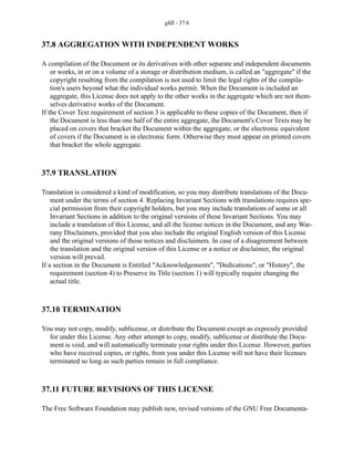
Figure 4.26 Dielectric Constants of Various Materials [Turck Proximity Sensors Guide]
The range and accuracy of these sensors are determined mainly by their size.
Larger sensors can have diameters of a few centimeters. Smaller ones can be less than a
centimeter across, and have smaller ranges, but more accuracy.
4.3.5 Inductive Sensors
Inductive sensors use currents induced by magnetic fields to detect nearby metal
objects. The inductive sensor uses a coil (an inductor) to generate a high frequency mag-
netic field as shown in Figure 4.27. If there is a metal object near the changing magnetic
field, current will flow in the object. This resulting current flow sets up a new magnetic
field that opposes the original magnetic field. The net effect is that it changes the induc-
tance of the coil in the inductive sensor. By measuring the inductance the sensor can deter-
mine when a metal have been brought nearby.
These sensors will detect any metals, when detecting multiple types of metal mul-
tiple sensors are often used.
Material
quartz glass
rubber
salt
sand
shellac
silicon dioxide
silicone rubber
silicone varnish
styrene resin
sugar
sugar, granulated
sulfur
sulfuric acid
Constant
3.7
2.5-35
6.0
3-5
2.0-3.8
4.5
3.2-9.8
2.8-3.3
2.3-3.4
3.0
1.5-2.2
3.4
84
Material
Teflon (TM), PCTFE
Teflon (TM), PTFE
toluene
trichloroethylene
urea resin
urethane
vaseline
water
wax
wood, dry
wood, pressed board
wood, wet
xylene
Constant
2.3-2.8
2.0
2.3
3.4
6.2-9.5
3.2
2.2-2.9
48-88
2.4-6.5
2-7
2.0-2.6
10-30
2.4](https://image.slidesharecdn.com/plc-programmable-logic-controller-book-230318130132-22ebd54b/85/PLC-Programmable-Logic-Controller-Book-pdf-87-320.jpg)
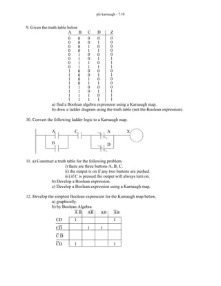

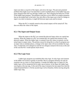


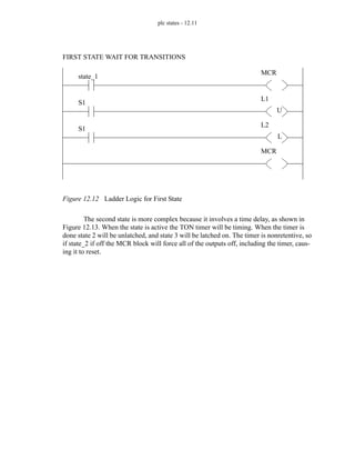
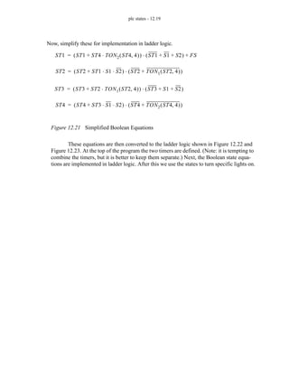

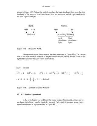
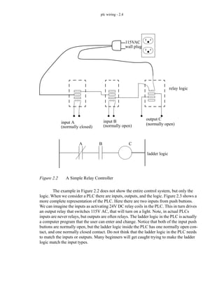
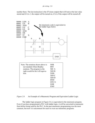
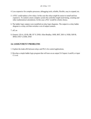
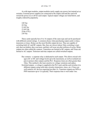
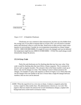
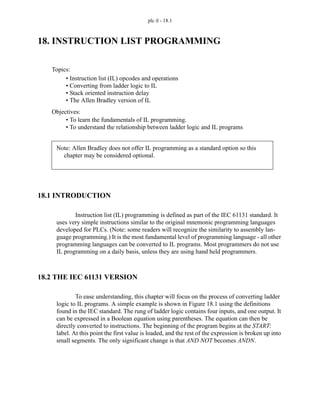
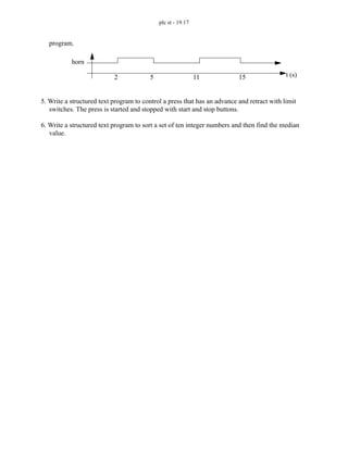
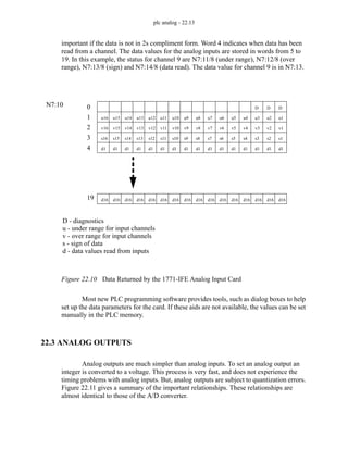
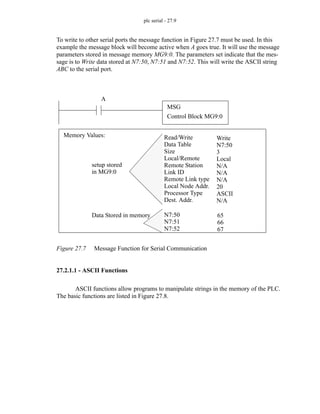
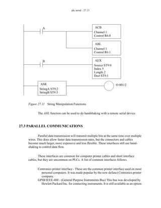
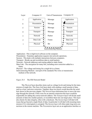
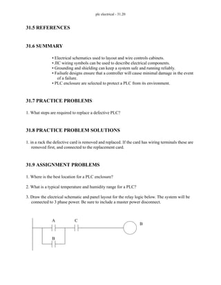
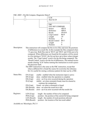
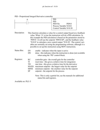
![plc numbers - 13.13
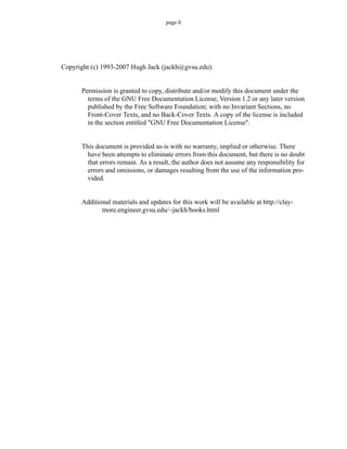
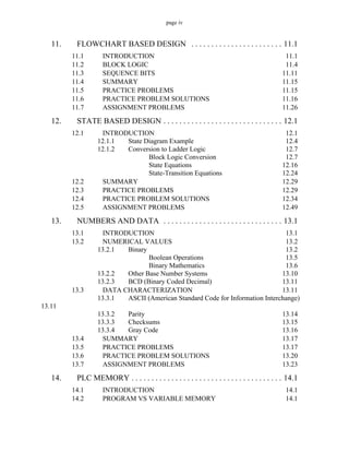
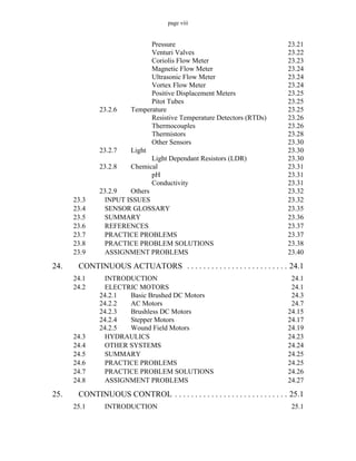
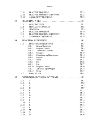
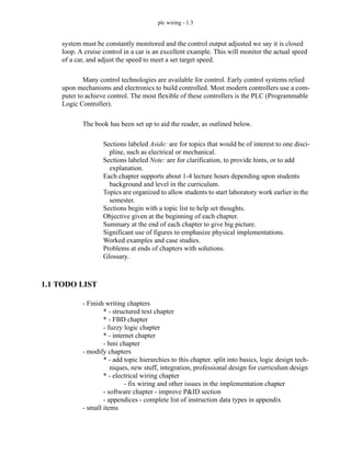
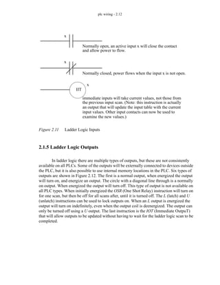
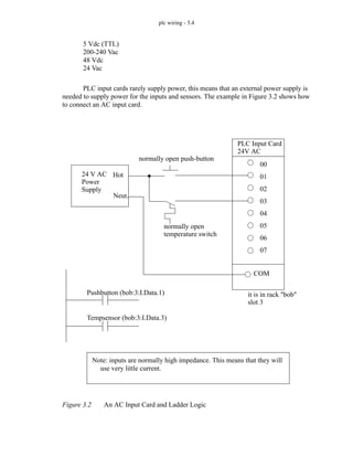
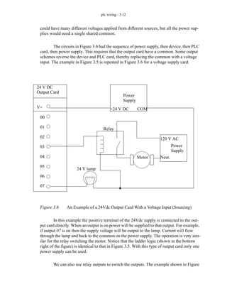
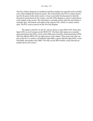
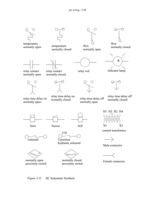
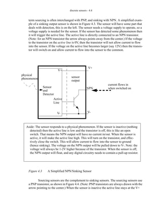
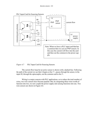
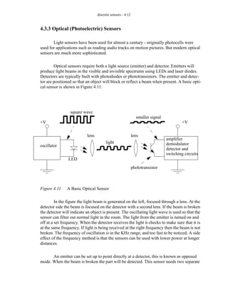
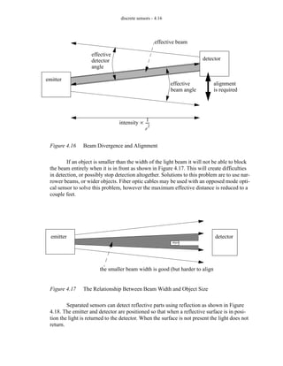
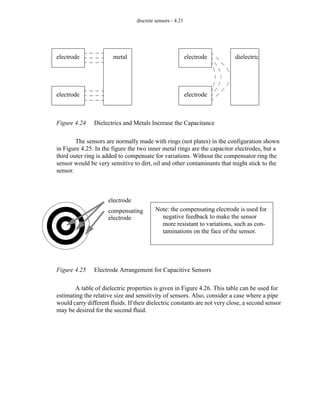
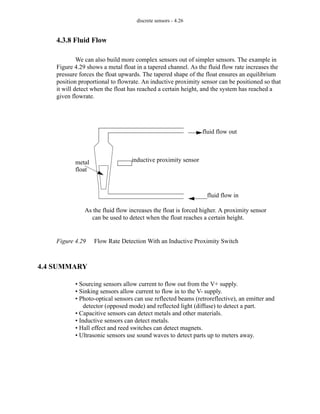
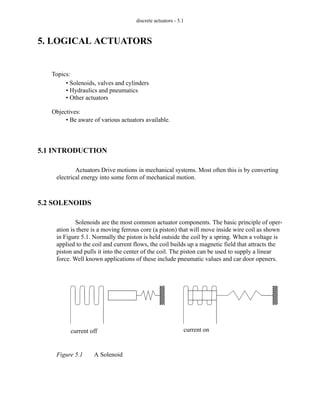
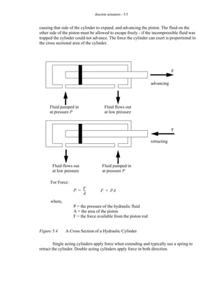
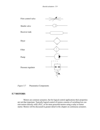
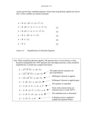
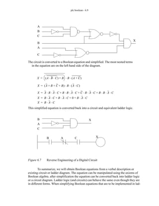
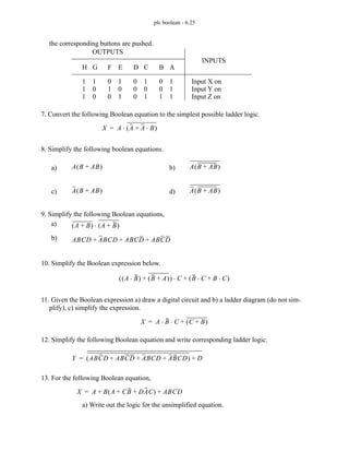
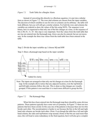
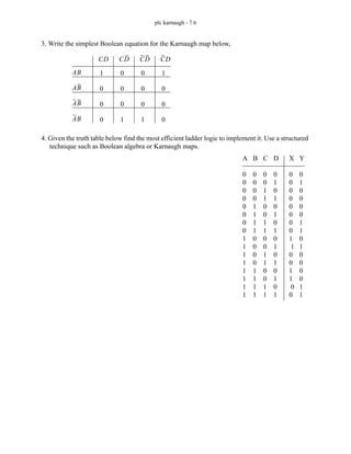
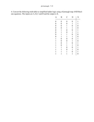
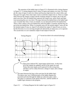
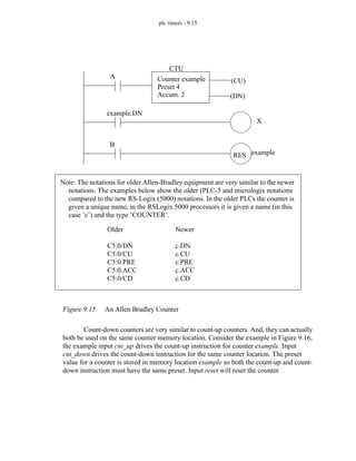
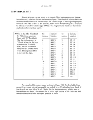
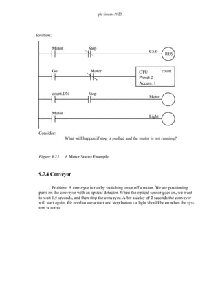
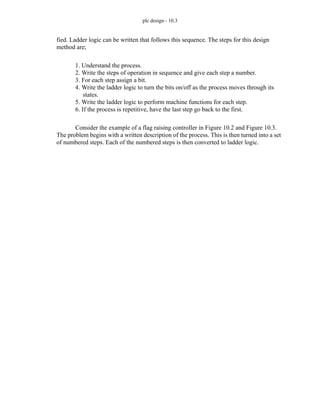
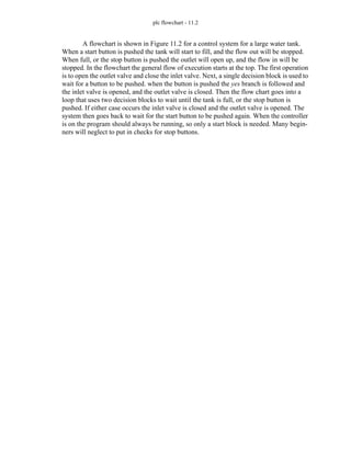
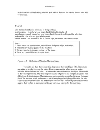
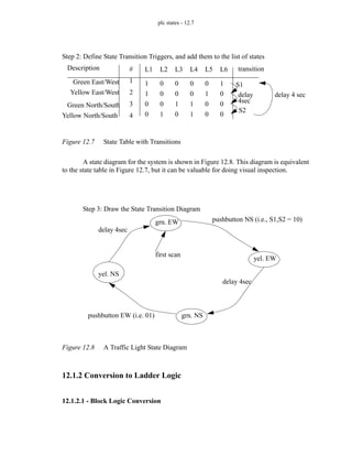
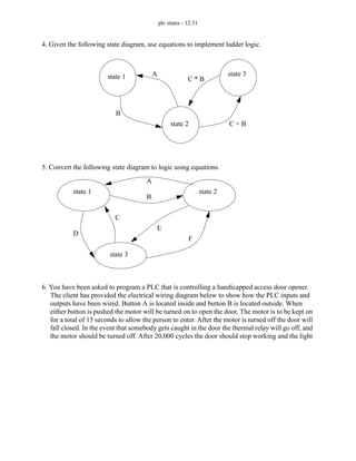
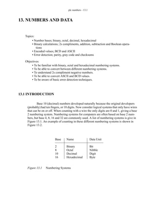
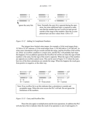
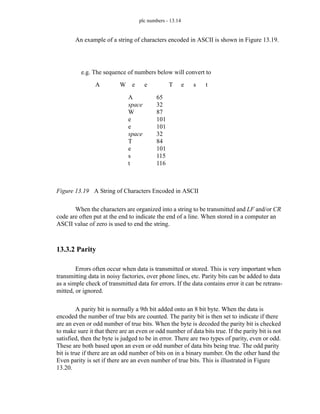
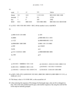
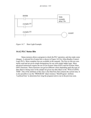
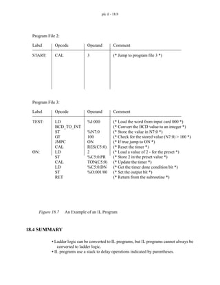
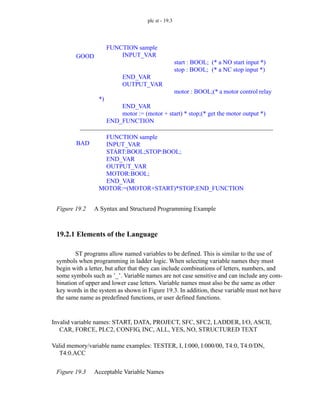
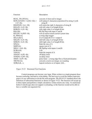
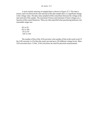
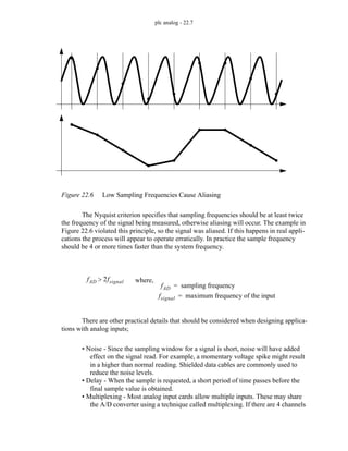
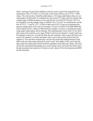
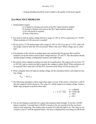
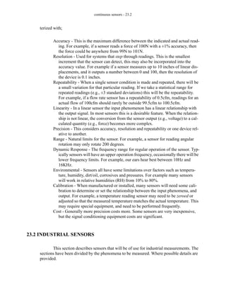
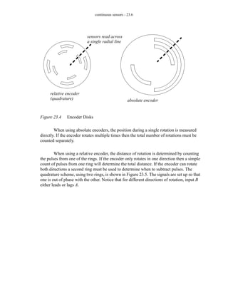
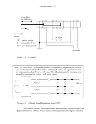
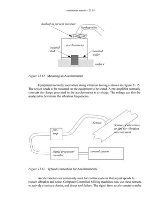
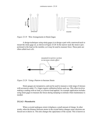
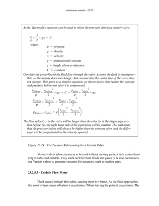
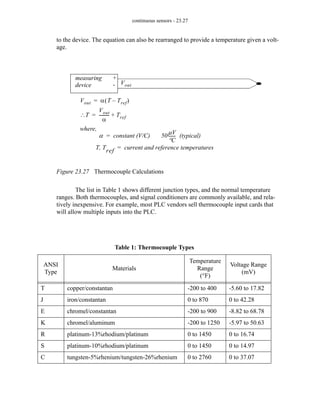
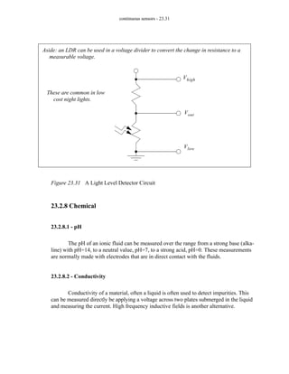
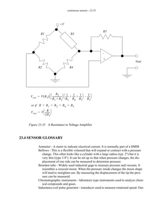
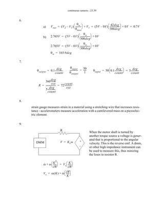
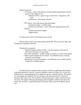
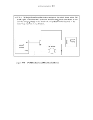
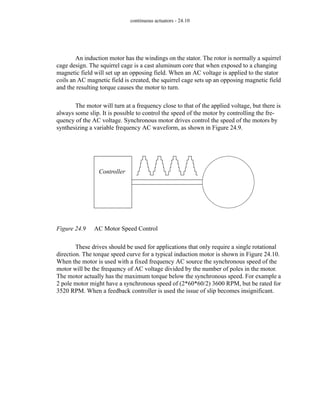
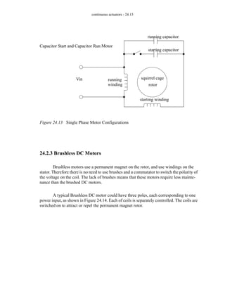
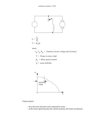
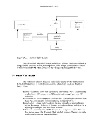
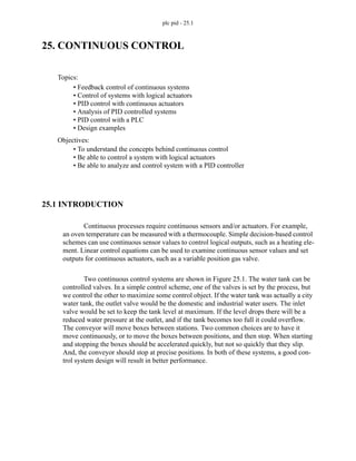
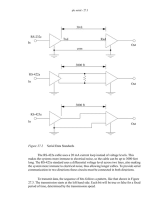
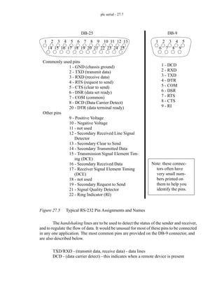
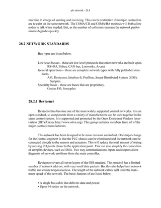
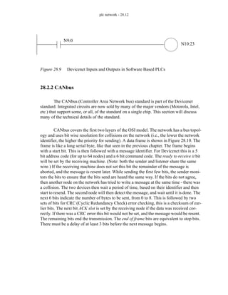
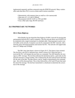
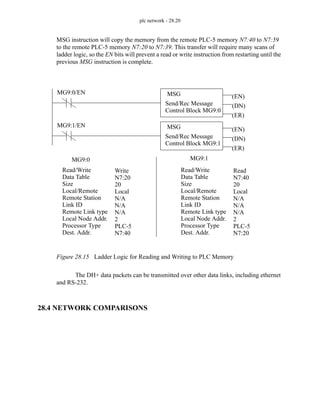
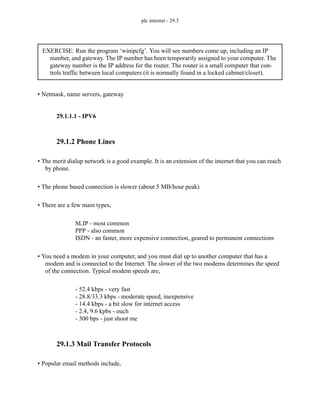
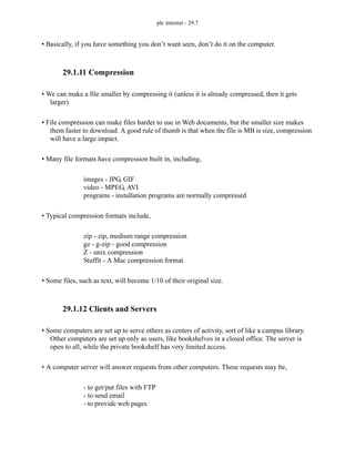
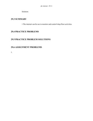
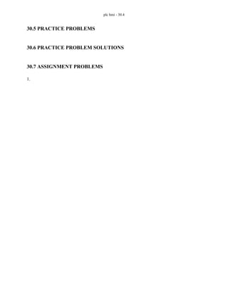
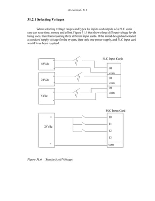
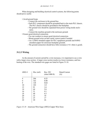
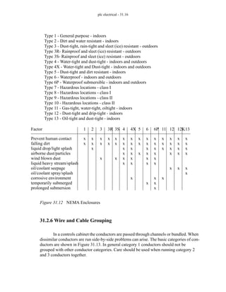
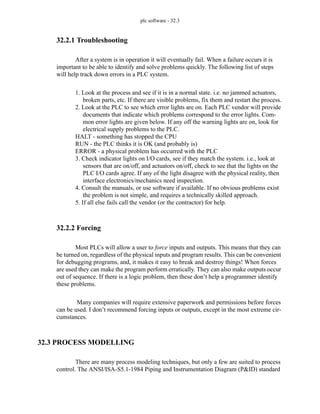
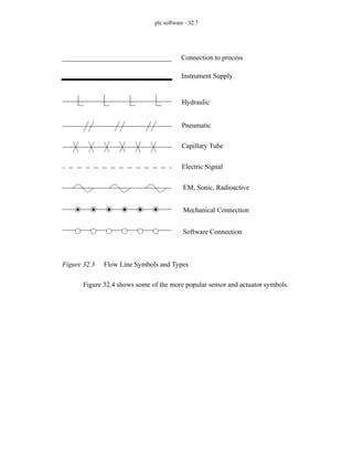
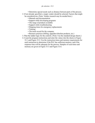
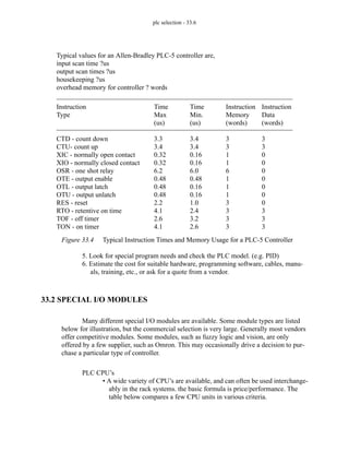
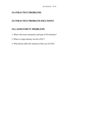
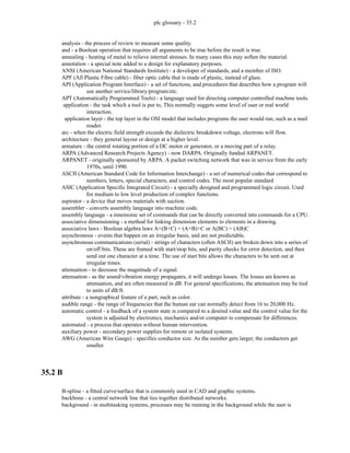
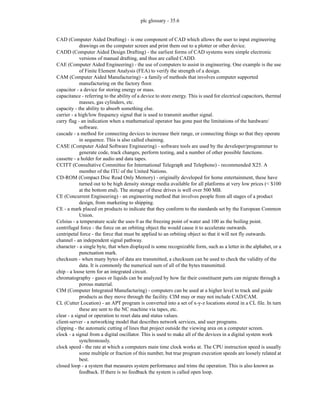
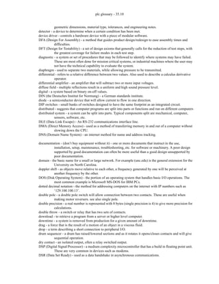
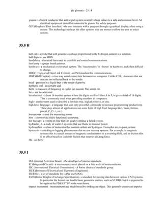
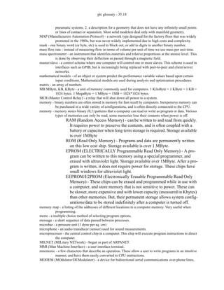
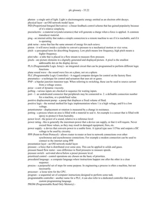
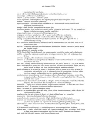
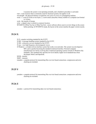
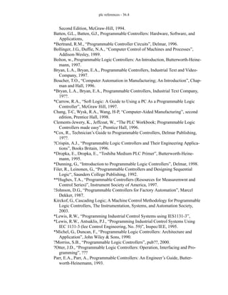
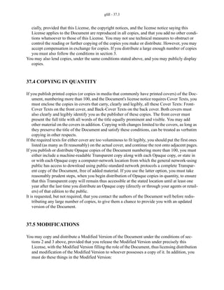
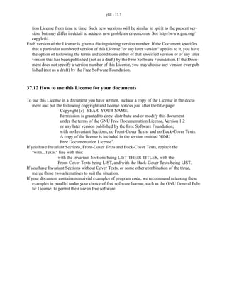
Figure 13.18 ASCII Character Table
This table has the codes from 0 to 127, but there are more extensive tables that
contain special graphics symbols, international characters, etc. It is best to use the basic
codes, as they are supported widely, and should suffice for all controls tasks.
64
65
66
67
68
69
70
71
72
73
74
75
76
77
78
79
80
81
82
83
84
85
86
87
88
89
90
91
92
93
94
95
40
41
42
43
44
45
46
47
48
49
4A
4B
4C
4D
4E
4F
50
51
52
53
54
55
56
57
58
59
5A
5B
5C
5D
5E
5F
01000000
01000001
01000010
01000011
01000100
01000101
01000110
01000111
01001000
01001001
01001010
01001011
01001100
01001101
01001110
01001111
01010000
01010001
01010010
01010011
01010100
01010101
01010110
01010111
01011000
01011001
01011010
01011011
01011100
01011101
01011110
01011111
@
A
B
C
D
E
F
G
H
I
J
K
L
M
N
O
P
Q
R
S
T
U
V
W
X
Y
Z
[
yen
]
^
_
decimal
hexadecimal
binary
ASCII
96
97
98
99
100
101
102
103
104
105
106
107
108
109
110
111
112
113
114
115
116
117
118
119
120
121
122
123
124
125
126
127
60
61
62
63
64
65
66
67
68
69
6A
6B
6C
6D
6E
6F
70
71
72
73
74
75
76
77
78
79
7A
7B
7C
7D
7E
7F
01100000
01100001
01100010
01100011
01100100
01100101
01100110
01100111
01101000
01101001
01101010
01101011
01101100
01101101
01101110
01101111
01110000
01110001
01110010
01110011
01110100
01110101
01110110
01110111
01111000
01111001
01111010
01111011
01111100
01111101
01111110
01111111
‘
a
b
c
d
e
f
g
h
i
j
k
l
m
n
o
p
q
r
s
t
u
v
w
x
y
z
{
|
}
r arr.
l arr.
decimal
hexadecimal
binary
ASCII](https://image.slidesharecdn.com/plc-programmable-logic-controller-book-230318130132-22ebd54b/85/PLC-Programmable-Logic-Controller-Book-pdf-338-320.jpg)
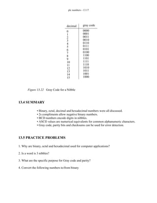
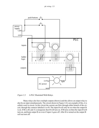
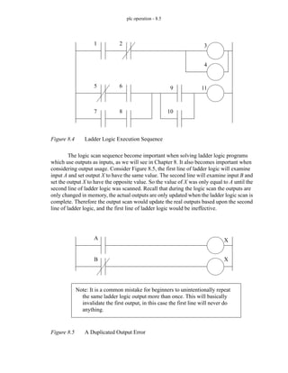
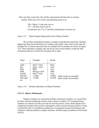
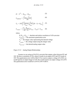
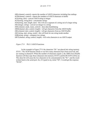
![plc memory - 14.5
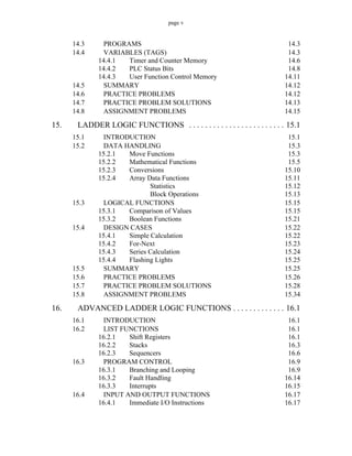
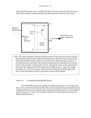
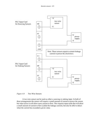
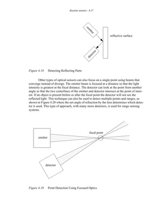
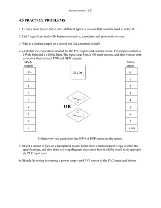
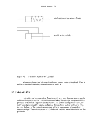
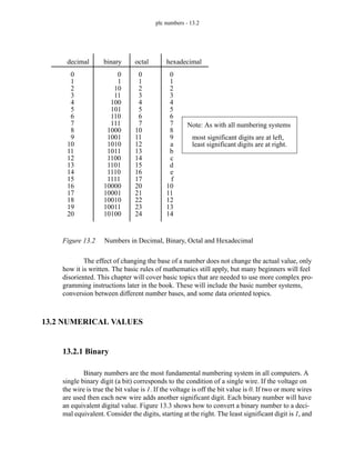
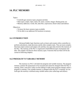
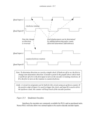
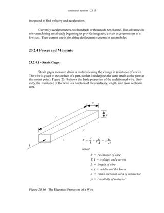
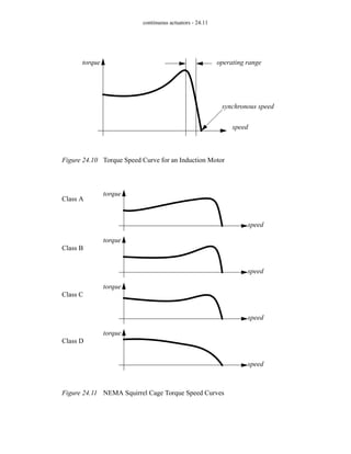
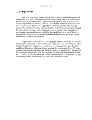
Figure 14.2 Literal Data Values
Data types can be created in variable size 1D, 2D, or 3D arrays.
Sometimes we will want to refer to an array of values, as shown in Figure 14.3.
This data type is indicated by beginning the number with a pound or hash sign ’#’. The
first example describes an array of floating point numbers staring in file 8 at location 5.
The second example is for an array of integers in file 7 starting at location 0. The length of
the array is determined elsewhere.
Figure 14.3 Arrays
Expressions allow addresses and functions to be typed in and interpreted when the
program is run. The example in Figure 14.4 will get a floating point number from ’test’,
perform a sine transformation, and then add 1.3. The text string is not interpreted until the
PLC is running, and if there is an error, it may not occur until the program is running - so
use this function cautiously.
Figure 14.4 Expressions
These data types and addressing modes will be discussed more as applicable func-
tions are presented later in this chapter and book.
8 - an integer
8.5 - a floating point number
08FH - a hexadecimal value 8F
01101101B - a binary number 01101101
test[1, 4] - returns the value in the 2nd row and 5th column of array test
“sin(test) + 1.3” - a simple calculation
expression - a text string that describes a complex operation.](https://image.slidesharecdn.com/plc-programmable-logic-controller-book-230318130132-22ebd54b/85/PLC-Programmable-Logic-Controller-Book-pdf-353-320.jpg)
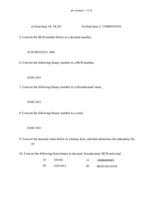
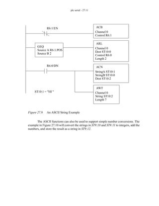
![plc memory - 14.9
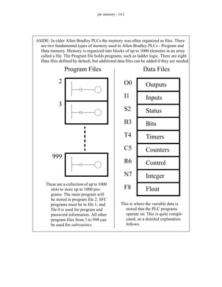
Figure 14.8 Status Bits and Words for ControlLogix
An example of getting and setting system status values is shown in Figure 14.9.
The first line of ladder logic will get the current time from the class ’WALLCLOCK-
TIME’. In this case the class does not have an instance so it is blank. The attribute being
recalled is the DateTime that will be written to the DINT array time[0..6]. For example
’time[3]’ should give the current hour. In the second line the Watchdog time for the Main-
Program is set to 200 ms. If the program MainProgram takes longer than 200ms to execute
S:FS - First Scan Flag
S:N - The last calculation resulted in a negative value
S:Z - The last calculation resulted in a zero
S:V - The last calculation resulted in an overflow
S:C - The last calculation resulted in a carry
S:MINOR - A minor (non-critical/recoverable) error has occurred
CONTROLLERDEVICE - information about the PLC
PROGRAM - information about the program running
LastScanTime
MaxScanTime
TASK
EnableTimeout
LastScanTime
MaxScanTime
Priority
StartTime
Watchdog
WALLCLOCKTIME - the current time
DateTime
DINT[0] - year
DINT[1] - month 1=january
DINT[2] - day 1 to 31
DINT[3] - hour 0 to 24
DINT[4] - minute 0 to 59
DINT[5] - second 0 to 59
DINT[6] - microseconds 0 to 999,999
Immediately accessible status values
Examples of SOME values available using the GSV and SSV functions](https://image.slidesharecdn.com/plc-programmable-logic-controller-book-230318130132-22ebd54b/85/PLC-Programmable-Logic-Controller-Book-pdf-357-320.jpg)
![plc memory - 14.10
a fault will be generated.
Figure 14.9 Reading and Setting Status bits with GSV and SSV
As always, additional classes and attributes for the status values can be found in
the manuals for the processors and instructions being used.
GSV
Class Name: WALLCLOCKTIME
Instance Name:
Attribute Name: DateTime
Dest: time[0]
SSV
Class Name: TASK
Instance Name: MainProgram
Attribute Name: Watchdog
Source: 200](https://image.slidesharecdn.com/plc-programmable-logic-controller-book-230318130132-22ebd54b/85/PLC-Programmable-Logic-Controller-Book-pdf-358-320.jpg)
![plc memory - 14.12
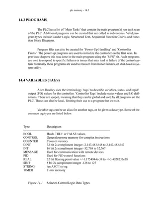
Figure 14.10 Bits and Words for Control Memory
14.5 SUMMARY
• Program are given unique names and can be for power-up, regular scans, and
faults.
• Tags and aliases are used for naming variables and I/O.
• Files are like arrays and are indicated with [].
• Expressions allow equations to be typed in.
• Literal values for binary and hexadecimal values are followed by B and H.
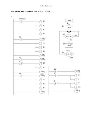
14.6 PRACTICE PROBLEMS
1. How are timer and counter memory similar?
2. What types of memory cannot be changed?
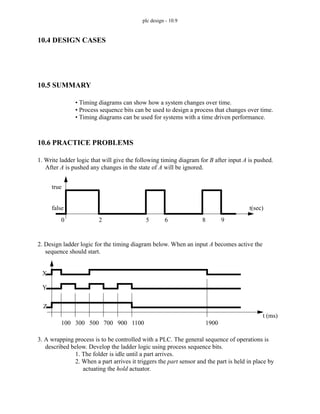
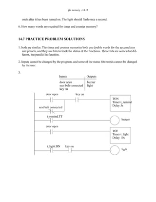
3. Develop Ladder Logic for a car door/seat belt safety system. When the car door is open, or the
seatbelt is not done up, a buzzer will sound for 5 seconds if the key has been switched on. A
cabin light will be switched on when the door is open and stay on for 10 seconds after it is
closed, unless a key has started the ignition power.
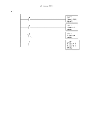
4. Write ladder logic for the following problem description. When button A is pressed a value of
1001 will be stored in X. When button B is pressed a value of -345 will be stored in Y, when it
is not pressed a value of 99 will be stored in Y. When button C is pressed X and Y will be added,
and the result will be stored in Z.
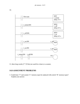
5. Using the status memory locations, write a program that will flash a light for the first 15 sec-
EN - enable bit
EU - enable unload
DN - done bit
EM - empty bit
ER - error bit
UL - unload bit
IN - inhibit bit
FD - found bit
LEN - length word
POS - position word](https://image.slidesharecdn.com/plc-programmable-logic-controller-book-230318130132-22ebd54b/85/PLC-Programmable-Logic-Controller-Book-pdf-360-320.jpg)
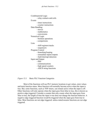
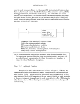
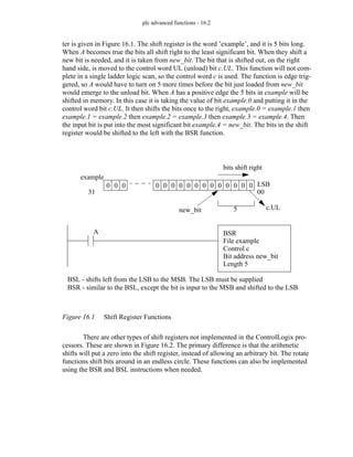
![plc basic functions - 15.11
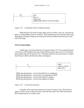
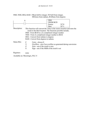
Figure 15.10 Conversion Example
15.2.4 Array Data Functions
Arrays allow us to store multiple data values. In a PLC this will be a sequential
series of numbers in integer, floating point, or other memory. For example, assume we are
measuring and storing the weight of a bag of chips in floating point memory starting at
weight[0]. We could read a weight value every 10 minutes, and once every hour find the
average of the six weights. This section will focus on techniques that manipulate groups of
data organized in arrays, also called blocks in the manuals.
FRD
Source bcd_1
Dest. int_0
TOD
Source int_1
Dest. bcd_0
DEG
Source real_0
Dest. real_2
RAD
Source real_1
Dest. real_3
Addr.
int_0
int_1
real_0
real_1
real_2
real_3
bcd_0
bcd_1
Before
0
548
3.141
45
0
0
0000 0000 0000 0000
0001 0111 1001 0011
after
1793
548
3.141
45
180
0.785
0000 0101 0100 1000
0001 0111 1001 0011
these are shown in
binary BCD form](https://image.slidesharecdn.com/plc-programmable-logic-controller-book-230318130132-22ebd54b/85/PLC-Programmable-Logic-Controller-Book-pdf-374-320.jpg)
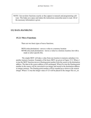
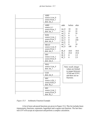
![plc basic functions - 15.12
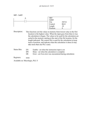
15.2.4.1 - Statistics
Functions are available that allow statistical calculations. These functions are
listed in Figure 15.11. When A becomes true the average (AVE) conversion will start at
memory location weight[0] and average a total of 4 values. The control word
weight_control is used to keep track of the progress of the operation, and to determine
when the operation is complete. This operation, and the others, are edge triggered. The
operation may require multiple scans to be completed. When the operation is done the
average will be stored in weight_avg and the weight_control.DN bit will be turned on.
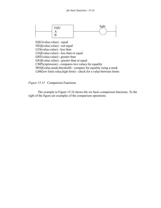
Figure 15.11 Statistic Functions
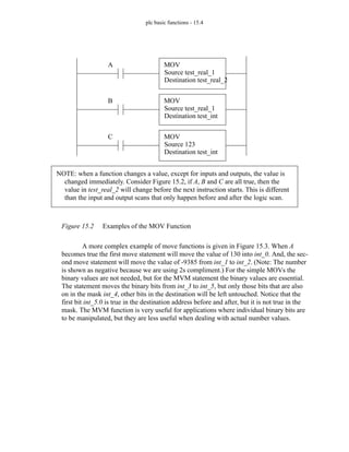
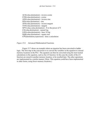
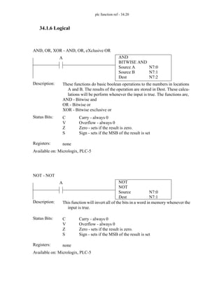
Examples of the statistical functions are given in Figure 15.12 for an array of data
that starts at weight[0] and is 4 values long. When done the average will be stored in
weight_avg, and the standard deviation will be stored in weight_std. The set of values will
also be sorted in ascending order from weight[0] to weight[3]. Each of the function should
have their own control memory to prevent overlap. It is not a good idea to activate the sort
and the other calculations at the same time, as the sort may move values during the calcu-
lation, resulting in incorrect calculations.
AVE(start value,destination,control,length) - average of values
STD(start value,destination,control,length) - standard deviation of values
SRT(start value,control,length) - sort a list of values
AVE
File weight[0]
Dest weight_avg
Control weight_control
length 4
position 0
A](https://image.slidesharecdn.com/plc-programmable-logic-controller-book-230318130132-22ebd54b/85/PLC-Programmable-Logic-Controller-Book-pdf-375-320.jpg)
![plc basic functions - 15.13
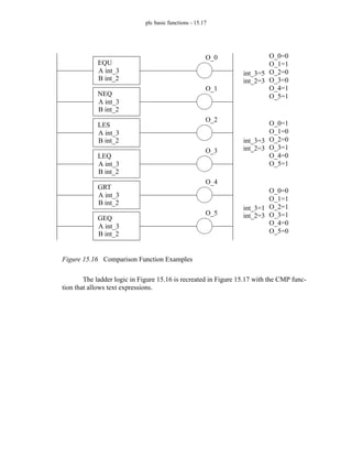
Figure 15.12 Statistical Calculations
15.2.4.2 - Block Operations
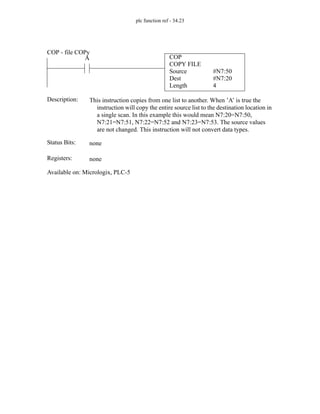
A basic block function is shown in Figure 15.13. This COP (copy) function will
AVE
File weight[0]
Dest weight_avg
Control c_1
length 4
position 0
STD
File weight[0]
Dest weight_std
Control c_2
length 4
position 0
SRT
File weight[0]
Control c_3
length 4
position 0
Addr.
weight[0]
weight[1]
weight[2]
weight[3]
weight_avg
weight_std
before
3
1
2
4
0
0
after A
3
1
2
4
2.5
0
A
B
C
after B
3
1
2
4
2.5
1.29
after C
1
2
3
4
2.5
1.29
ASIDE: These function will allow a real-time calculation of SPC data for con-
trol limits, etc. The only PLC function missing is a random function that
would allow random sample times.](https://image.slidesharecdn.com/plc-programmable-logic-controller-book-230318130132-22ebd54b/85/PLC-Programmable-Logic-Controller-Book-pdf-376-320.jpg)
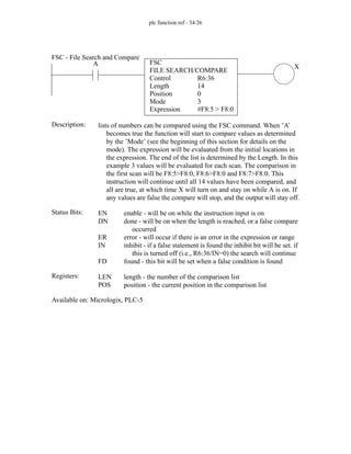
![plc basic functions - 15.14
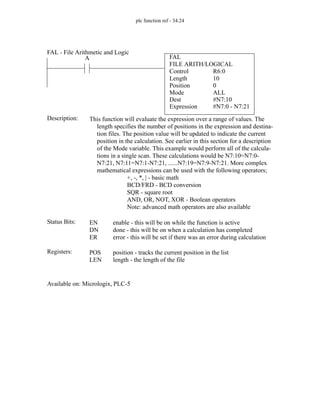
copy an array of 10 values starting at n[50] to n[40]. The FAL function will perform math-
ematical operations using an expression string, and the FSC function will allow two arrays
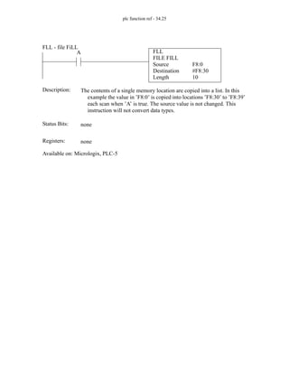
to be compared using an expression. The FLL function will fill a block of memory with a
single value.
Figure 15.13 Block Operation Functions
Figure 15.14 shows an example of the FAL function with different addressing
modes. The first FAL function will do the following calculations n[5]=n[0]+5,
n[6]=n[1]+5, n[7]=n[2]+5, n[7]=n[3]+5, n[9]=n[4]+5. The second FAL statement will
be n[5]=n[0]+5, n[6]=n[0]+5, n[7]=n[0]+5, n[7]=n[0]+5, n[9]=n[0]+5. With a mode
of 2 the instruction will do two of the calculations when there is a positive edge from B
(i.e., a transition from false to true). The result of the last FAL statement will be
n[5]=n[0]+5, n[5]=n[1]+5, n[5]=n[2]+5, n[5]=n[3]+5, n[5]=n[4]+5. The last opera-
tion would seem to be useless, but notice that the mode is incremental. This mode will do
one calculation for each positive transition of C. The all mode will perform all five calcu-
lations in a single scan whenever there is a positive edge on the input. It is also possible to
put in a number that will indicate the number of calculations per scan. The calculation
time can be long for large arrays and trying to do all of the calculations in one scan may
lead to a watchdog time-out fault.
COP(start value,destination,length) - copies a block of values
FAL(control,length,mode,destination,expression) - will perform basic math
operations to multiple values.
FSC(control,length,mode,expression) - will do a comparison to multiple values
FLL(value,destination,length) - copies a single value to a block of memory
COP
Source n[50]
Dest n[40]
Length 10
A](https://image.slidesharecdn.com/plc-programmable-logic-controller-book-230318130132-22ebd54b/85/PLC-Programmable-Logic-Controller-Book-pdf-377-320.jpg)
![plc basic functions - 15.15
Figure 15.14 File Algebra Example
15.3 LOGICAL FUNCTIONS
15.3.1 Comparison of Values
Comparison functions are shown in Figure 15.15. Previous function blocks were
outputs, these replace input contacts. The example shows an EQU (equal) function that
compares two floating point numbers. If the numbers are equal, the output bit light is true,
otherwise it is false. Other types of equality functions are also listed.
FAL
Control c_0
length 5
position 0
Mode all
Destination n[c_0.POS + 5]
Expression n[c_0.POS] + 5
FAL
Control R6:1
length 5
position 0
Mode 2
Destination n[c_0.POS + 5]
Expression n[0] + 5
array to array
element to array
array to element
FAL
Control R6:2
length 5
position 0
Mode incremental
Destination n[5]
Expression n[c_0.POS] + 5
array to element
A
B
C](https://image.slidesharecdn.com/plc-programmable-logic-controller-book-230318130132-22ebd54b/85/PLC-Programmable-Logic-Controller-Book-pdf-378-320.jpg)
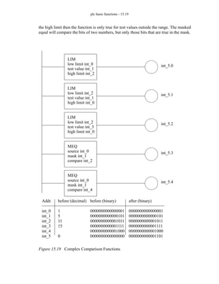
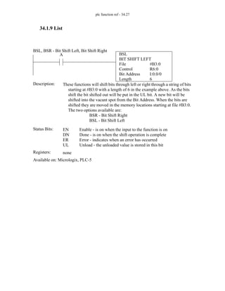
![plc basic functions - 15.20
Figure 15.20 shows a numberline that helps determine when the LIM function will
be true.
Figure 15.20 A Number Line for the LIM Function
File to file comparisons are also permitted using the FSC instruction shown in Fig-
ure 15.21. The instruction uses the control word c_0. It will interpret the expression 10
times, doing two comparisons per logic scan (the Mode is 2). The comparisons will be
f[10]<f[0], f[11]<f[0] then f[12]<f[0], f[13]<f[0] then f[14]<f[0], f[15]<f[0] then
f[16]<f[0], f[17]<f[0] then f[18]<f[0], f[19]<f[0]. The function will continue until a
false statement is found, or the comparison completes. If the comparison completes with
no false statements the output A will then be true. The mode could have also been All to
execute all the comparisons in one scan, or Increment to update when the input to the
function is true - in this case the input is a plain wire, so it will always be true.
Figure 15.21 File Comparison Using Expressions
high limit
low limit
low limit
high limit
FSC
Control c_0
Length 10
Position 0
Mode 2
Expression f[10+c_0.POS] < f[0]
A](https://image.slidesharecdn.com/plc-programmable-logic-controller-book-230318130132-22ebd54b/85/PLC-Programmable-Logic-Controller-Book-pdf-383-320.jpg)
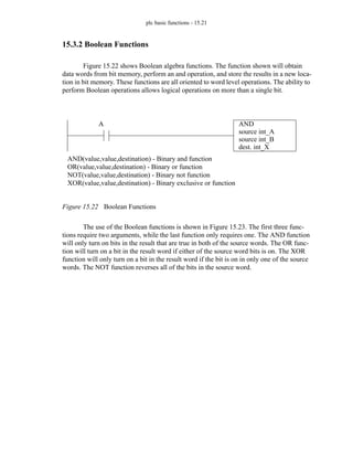
![plc basic functions - 15.22
Figure 15.23 Boolean Function Example
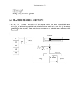
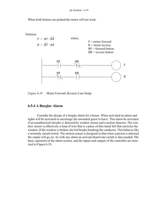
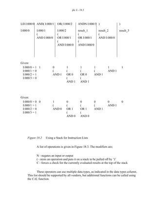
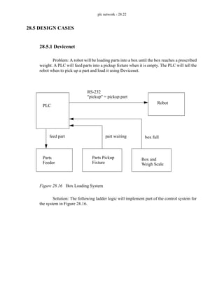
15.4 DESIGN CASES
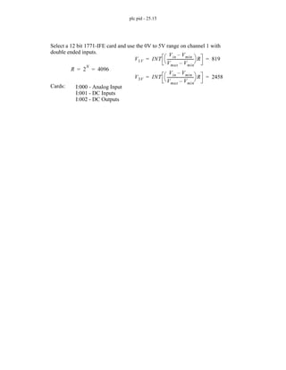
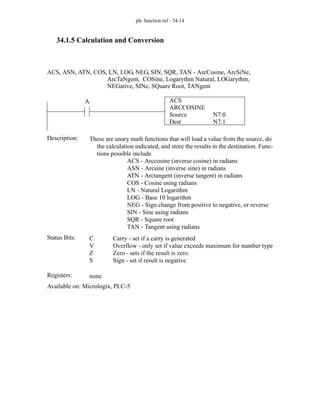
15.4.1 Simple Calculation
Problem: A switch will increment a counter on when engaged. This counter can be
reset by a second switch. The value in the counter should be multiplied by 2, and then dis-
played as a BCD output using (O:0.0/0 - O:0.0/7)
AND
source A n[0]
source B n[1]
dest. n[2]
OR
source A n[0]
source B n[1]
dest. n[3]
XOR
source A n[0]
source B n[1]
dest. n[4]
NOT
source A n[0]
dest. n[5]
n[0]
n[1]
n[2]
n[3]
n[4]
n[5]
0011010111011011
1010010011101010
0010010011001010
1011010111111011
1001000100110001
1100101000100100
addr. data (binary)
after](https://image.slidesharecdn.com/plc-programmable-logic-controller-book-230318130132-22ebd54b/85/PLC-Programmable-Logic-Controller-Book-pdf-385-320.jpg)
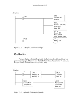
![plc basic functions - 15.25
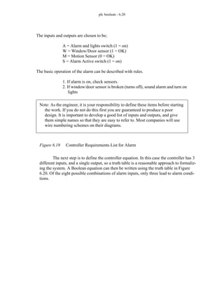
15.4.4 Flashing Lights
Problem: We are designing a movie theater marquee, and they want the traditional
flashing lights. The lights have been connected to the outputs of the PLC from O[0] to
O[17] - an INT. When the PLC is turned, every second light should be on. Every half sec-
ond the lights should reverse. The result will be that in one second two lights side-by-side
will be on half a second each.
Figure 15.27 A Flashing Light Example
15.5 SUMMARY
• Functions can get values from memory, do simple operations, and return the
results to memory.
• Scientific and statistics math functions are available.
• Masked function allow operations that only change a few bits.
• Expressions can be used to perform more complex operations.
• Conversions are available for angles and BCD numbers.
• Array oriented file commands allow multiple operations in one scan.
TON
timer t_a
Delay 0.5s
TON
timer t_b
Delay 0.5s
t_b.DN
t_a.DN
MOV
Source pattern
Dest O
t_a.TT
NOT
Source pattern
Dest O
t_a.TT
pattern = 0101 0101 0101 0101
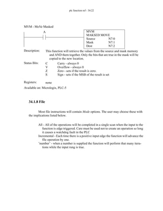
Solution:](https://image.slidesharecdn.com/plc-programmable-logic-controller-book-230318130132-22ebd54b/85/PLC-Programmable-Logic-Controller-Book-pdf-388-320.jpg)
![plc basic functions - 15.26
• Values can be compared to make decisions.
• Boolean functions allow bit level operations.
• Function change value in data memory immediately.
15.6 PRACTICE PROBLEMS
1. Do the calculation below with ladder logic,
2. Implement the following function,
3. A switch will increment a counter on when engaged. This counter can be reset by a second
switch. The value in the counter should be multiplied by 5, and then displayed as a binary out-
put using output integer ’O_lights’.
4. Create a ladder logic program that will start when input A is turned on and calculate the series
below. The value of n will start at 0 and with each scan of the ladder logic n will increase by 2
until n=20. While the sequence is being incremented, any change in A will be ignored.
5. The following program uses indirect addressing. Indicate what the new values in memory will
be when button A is pushed after the first and second instructions.
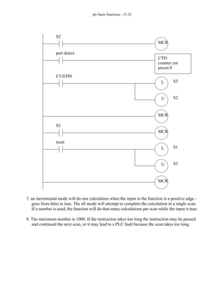
6. A thumbwheel input card acquires a four digit BCD count. A sensor detects parts dropping
n_2 = -(5 - n_0 / n_1)
x y
y y
( )
log
+
y 1
+
------------------------
⎝ ⎠
⎛ ⎞
⎝ ⎠
⎛ ⎞
atan
=
x 2 n
( )
log 1
–
( )
=
ADD
Source A 1
Source B n[0]
Dest. n[n[1]]
n[0]
n[1]
n[2]
1
addr before after 1st
2
ADD
Source A n[n[0]]
Source B n[n[1]]
Dest. n[n[0]]
A
A
3
after 2nd](https://image.slidesharecdn.com/plc-programmable-logic-controller-book-230318130132-22ebd54b/85/PLC-Programmable-Logic-Controller-Book-pdf-389-320.jpg)
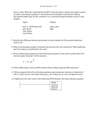
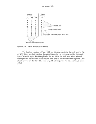
![plc basic functions - 15.30
5.
6.
n[0]
n[1]
n[2]
1
addr before after 1st
2
3
after 2nd
1 1
2
2
4
2
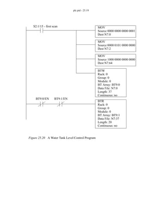
first scan
count
reset
waiting
parts
counting
bin
full
start
(chute open)
exceeded
(light on)
S1 S2
S3](https://image.slidesharecdn.com/plc-programmable-logic-controller-book-230318130132-22ebd54b/85/PLC-Programmable-Logic-Controller-Book-pdf-393-320.jpg)
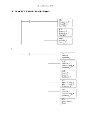
![plc basic functions - 15.34
11.
12.
15.8 ASSIGNMENT PROBLEMS
1. Write a ladder logic program that will implement the function below, and if the result is greater
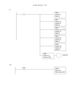
than 100.5 then the output ’too_hot’ will be turned on.
2. Use an FAL instruction to average the values in n[0] to n[20] and store them in ’n_avg’.
3. Write some simple ladder logic to change the preset value of a counter. When the input ‘A’ is
active the preset should be 13, otherwise it will be 9.
4. The 16 input bits from ’input_card_A’ are to be read and XORed with the inputs from
’input_card_B’. The result is to be written to the output card ’output_card’. If the binary pat-
tern of the outputs is 1010 0101 0111 0110 then the output ’match_bell’ will be set. Write the
ladder logic.
5. A machine ejects parts into three chutes. Three optical sensors (A, B and C) are positioned in
each of the slots to count the parts. The count should start when the reset (R) button is pushed.
The count will stop, and an indicator light (L) turned on when the average number of parts
counted as 100 or greater.
6. Write ladder logic to calculate the average of the values from thickness[0] to thickness[99]. The
operation should start after a momentary contact push button A is pushed. The result should be
AND
Source A input_card
Source B 0000 0010 0001 0100 (binary)
Dest temp
EQU
Source A 0000 0010 0001 0100 (binary)
Source B temp
match
D = (S & M) + (D & M)
The data in the source location will be moved bit by bit to the destination for every bit
that is set in the mask. Every other bit in the destination will be retain the pre-
vious value. The source address is not changed.
X 6 Ae
B
C 5
+
( )
cos
+
=](https://image.slidesharecdn.com/plc-programmable-logic-controller-book-230318130132-22ebd54b/85/PLC-Programmable-Logic-Controller-Book-pdf-397-320.jpg)
![plc basic functions - 15.35
stored in ’thickness_avg’. If button B is pushed, all operations should be complete in a single
scan. Otherwise, only ten values will be calculated each scan. (Note: this means that it will take
10 scans to complete the calculation if A is pushed.)
7. Write and simplify a Boolean equation that implements the masked move (MVM) instruction.
The source is S, the mask is M and the destination is D.
8. a) Write ladder logic to calculate and store the binary sequence in 32 bit integer (DINT) mem-
ory starting at n[0] up to n[200] so that n[0] = 1, n[1] = 2, n[2] = 4, n[3] = 8, n[4] = 16, etc. b)
Will the program operate as expected?](https://image.slidesharecdn.com/plc-programmable-logic-controller-book-230318130132-22ebd54b/85/PLC-Programmable-Logic-Controller-Book-pdf-398-320.jpg)
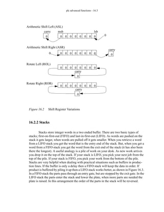
![plc advanced functions - 16.4
Figure 16.3 Buffers and Stack Types
The ladder logic functions are FFL to load the stack, and FFU to unload it. The
example in Figure 16.4 shows two instructions to load and unload a FIFO stack. The first
time this FFL is activated (edge triggered) it will grab the word (16 bits) from the input
card word_in and store them on the stack, at stack[0]. The next value would be stored at
stack[1], and so on until the stack length is reached at stack[4]. When the FFU is activated
the word at stack[0] will be moved to the output card word_out. The values on the stack
will be shifted up so that the value previously in stack[1] moves to stack[0], stack[2]
moves to stack[1], etc. If the stack is full or empty, an a load or unload occurs the error bit
will be set c.ER.
FIFO
LIFO
entry gate exit gate](https://image.slidesharecdn.com/plc-programmable-logic-controller-book-230318130132-22ebd54b/85/PLC-Programmable-Logic-Controller-Book-pdf-402-320.jpg)
![plc advanced functions - 16.5
Figure 16.4 FIFO Stack Instructions
The LIFO stack commands are shown in Figure 16.5. As values are loaded on the
stack the will be added sequentially stack[0], stack[1], stack[2], stack[3] then stack[4].
When values are unloaded they will be taken from the last loaded position, so if the stack
is full the value of stack[4] will be removed first.
Figure 16.5 LIFO Stack Commands
FFL
source word_in
FIFO stack[0]
Control c
length 5
position 0
FFU
FIFO stack[0]
destination word_out
Control c
length 5
position 0
A
B
LFL
source word_in
LIFO stack[0]
Control c
length 5
position 0
LFU
LIFO stack[0]
destination word_out
Control c
length 5
position 0
A
B](https://image.slidesharecdn.com/plc-programmable-logic-controller-book-230318130132-22ebd54b/85/PLC-Programmable-Logic-Controller-Book-pdf-403-320.jpg)
![plc advanced functions - 16.6
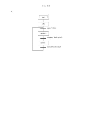
16.2.3 Sequencers
A mechanical music box is a simple example of a sequencer. As the drum in the
music box turns it has small pins that will sound different notes. The song sequence is
fixed, and it always follows the same pattern. Traffic light controllers are now controlled
with electronics, but previously they used sequencers that were based on a rotating drum
with cams that would open and close relay terminals. One of these cams is shown in Fig-
ure 16.6. The cam rotates slowly, and the surfaces under the contacts will rise and fall to
open and close contacts. For a traffic light controllers the speed of rotation would set the
total cycle time for the traffic lights. Each cam will control one light, and by adjusting the
circumferential length of rises and drops the on and off times can be adjusted.
Figure 16.6 A Single Cam in a Drum Sequencer
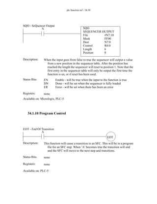
A PLC sequencer uses a list of words in memory. It recalls the words one at a time
and moves the words to another memory location or to outputs. When the end of the list is
reached the sequencer will return to the first word and the process begins again. A
sequencer is shown in Figure 16.7. The SQO instruction will retrieve words from bit
memory starting at sequence[0]. The length is 4 so the end of the list will be at
sequence[0]+4 or sequence[4] (the total length of ’sequence’ is actually 5). The sequencer
is edge triggered, and each time A becomes true the retrieve a word from the list and move
it to output_lights. When the sequencer reaches the end of the list the sequencer will return
to the second position in the list sequence[1]. The first item in the list is sequence[0], and
it will only be sent to the output if the SQO instruction is active on the first scan of the
PLC, otherwise the first word sent to the output is sequence[1]. The mask value is 000Fh,
or 0000000000001111b so only the four least significant bits will be transferred to the out-
put, the other output bits will not be changed. The other instructions allow words to be
added or removed from the sequencer list.
As the cam rotates it makes contact
with none, one, or two terminals, as
determined by the depressions and
rises in the rotating cam.](https://image.slidesharecdn.com/plc-programmable-logic-controller-book-230318130132-22ebd54b/85/PLC-Programmable-Logic-Controller-Book-pdf-404-320.jpg)
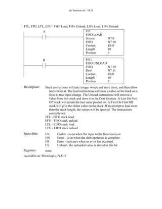
![plc advanced functions - 16.7
Figure 16.7 The Basic Sequencer Instruction
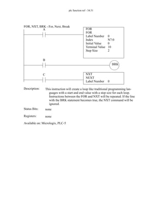
An example of a sequencer is given in Figure 16.8 for traffic light control. The
light patterns are stored in memory (entered manually by the programmer). These are then
moved out to the output card as the function is activated. The mask (003Fh =
0000000000111111b) is used so that only the 6 least significant bits are changed.
SQO(start,mask,destination,control,length) - sequencer output from table to memory
SQI(start,mask,source,control,length) - sequencer input from memory address to table
SQL(start,source,control,length) - sequencer load to set up the sequencer parameters
SQO
File sequence[0]
Mask 000F
Destination output_lights
Control c
Length 4
Position 0
A](https://image.slidesharecdn.com/plc-programmable-logic-controller-book-230318130132-22ebd54b/85/PLC-Programmable-Logic-Controller-Book-pdf-405-320.jpg)
![plc advanced functions - 16.8
Figure 16.8 A Sequencer For Traffic Light Control
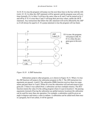
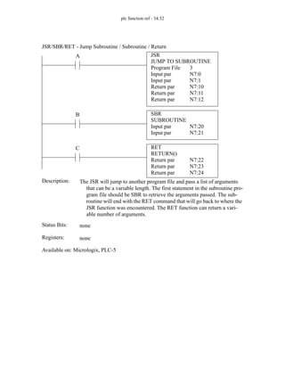
Figure 16.9 shows examples of the other sequencer functions. When A goes from
false to true, the SQL function will move to the next position in the sequencer list, for
example sequence_rem[1], and load a value from input_word. If A then remains true the
value in sequence_rem[1] will be overwritten each scan. When the end of the sequencer
list is encountered, the position will reset to 1.
The sequencer input (SQI) function will compare values in the sequence list to the
source compare_word while B is true. If the two values match match_output will stay on
while B remains true. The mask value is 0005h or 0000000000000101b, so only the first
and third bits will be compared. This instruction does not automatically change the posi-
tion, so logic is shown that will increment the position every scan while C is true.
SQO
File light_pattern
Mask 003Fh
Destination lights_output
Control c
Length 4
Position 0
0 0 0 0 0 0 0 0 0 0 0 0 1 1 0 0
0 0 0 0 0 0 0 0 0 0 0 0 1 0 1 0
0 0 0 0 0 0 0 0 0 0 1 0 0 0 0 1
0 0 0 0 0 0 0 0 0 0 0 1 0 0 0 1
light_pattern[0]
light_pattern[1]
NS
-
red
NS
-
yellow
NS
-
green
EW
-
red
EW
-
yellow
EW
-
green
0 0 0 0 0 0 0 0 0 0 0 0 1 0 0 1
advance](https://image.slidesharecdn.com/plc-programmable-logic-controller-book-230318130132-22ebd54b/85/PLC-Programmable-Logic-Controller-Book-pdf-406-320.jpg)
![plc advanced functions - 16.9
Figure 16.9 Sequencer Instruction Examples
These instructions are well suited to processes with a single flow of execution,
such as traffic lights.
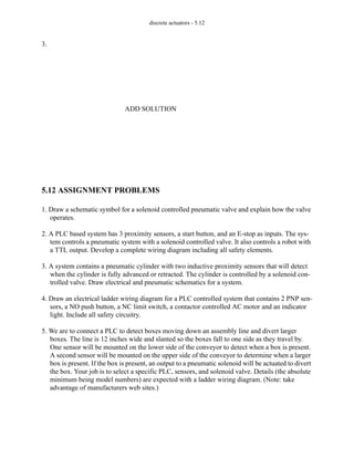
16.3 PROGRAM CONTROL
16.3.1 Branching and Looping
These functions allow parts of ladder logic programs to be included or excluded
from each program scan. These functions are similar to functions in other programming
languages such as C, C++, Java, Pascal, etc.
Entire sections of programs can be bypassed using the JMP instruction in Figure
SQI
File sequence_rem[0]
Mask 0005
Source compare_word
Control c_2
Length 9
Position 0
B
SQL
File sequence_rem[0]
Source input_word
Control c_1
Length 9
Position 0
A
match_output
ADD
SourceA c_2.POS
SourceB 1
Dest c_2.POS
C
MOV
Source 1
Dest c_2.POS
GT
SourceA c_2.POS
SourceB 9](https://image.slidesharecdn.com/plc-programmable-logic-controller-book-230318130132-22ebd54b/85/PLC-Programmable-Logic-Controller-Book-pdf-407-320.jpg)
![plc advanced functions - 16.14
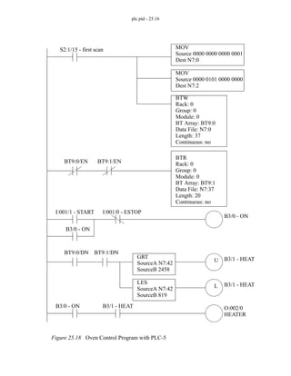
16.3.2 Fault Handling
A fault condition can stop a PLC. If the PLC is controlling a dangerous process
this could lead to significant damage to personnel and equipment. There are two types of
faults that occur; terminal (major) and warnings (minor). A minor fault will normally set
an error bit, but not stop the PLC. A major failure will normally stop the PLC, but an inter-
rupt can be used to run a program that can reset the fault bit in memory and continue oper-
ation (or shut down safely). Not all major faults are recoverable. A complete list of these
faults is available in PLC processor manuals.
The PLC can be set up to run a program when a fault occurs, such as a divide by
zero. These routines are program files under ’Control Fault Handler’. These routines will
be called when a fault occurs. Values are set in status memory to indicate the source of the
faults.
Figure 16.15 shows two example programs. The default program ’MainProgram’
will generate a fault, and the interrupt program called ’Recover’ will detect the fault and
fix it. When A is true a compute function will interpret the expression, using indirect
addressing. If B becomes true then the value in n[0] will become negative. If A becomes
true after this then the expression will become n[10] +10. The negative value for the
address will cause a fault, and program file ’Recover’ will be run.
In the fault program the fault values are read with an GSV function and the fault
code is checked. In this case the error will result in a status error of 0x2104. When this is
the case the n[0] is set back to zero, and the fault code in fault_data[2] is cleared. This
value is then written back to the status memory using an SSV function. If the fault was not
cleared the PLC would enter a fault state and stop (the fault light on the front of the PLC
will turn on).](https://image.slidesharecdn.com/plc-programmable-logic-controller-book-230318130132-22ebd54b/85/PLC-Programmable-Logic-Controller-Book-pdf-412-320.jpg)
![plc advanced functions - 16.15
Figure 16.15 A Fault Recovery Program
16.3.3 Interrupts
The PLC can be set up to run programs automatically using interrupts. This is rou-
tinely done for a few reasons;
• to run a program at a regular timed interval (e.g. SPC calculations)
CPT
Dest n[1]
Expression
n[n[0]] + 10
A
EQU
SourceA fault_data[2]
SourceB 0x2104
CLR
Dest. fault_data[2]
MainProgram
Recover
MOV
Source 0
Dest N7:0
MOV
Source -10
Dest n[0]
B
GSV
Object: PROGRAM
Instance: THIS
Attribute: MAJORFAULTRECORD
Dest: fault_data (Note: DINT[11])
SSV
Object: PROGRAM
Instance: THIS
Attribute: MAJORFAULTRECORD
Dest: fault_data](https://image.slidesharecdn.com/plc-programmable-logic-controller-book-230318130132-22ebd54b/85/PLC-Programmable-Logic-Controller-Book-pdf-413-320.jpg)
![plc advanced functions - 16.16
• to respond when a long instruction is complete (e.g. analog input)
• when a certain input changed (e.g. panic button)
Allen Bradley allows interrupts, but they are called periodic/event tasks. By
default the main program is defined as a ’continuous’ task, meaning that it runs as often as
possible, typically 10-100 times per second. Only one continuos task is allowed. A ’peri-
odic’ task can be created that has a given update time. ’Event’ tasks can be triggered by a
variety of actions, including input changes, tag changes, EVENT instructions, and servo
control changes.
A timed interrupt will run a program at regular intervals. To set a timed interrupt
the program in file number should be put in S2:31. The program will be run every S2:30
times 1 milliseconds. In Figure 16.16 program 2 will set up an interrupt that will run pro-
gram 3 every 5 seconds. Program 3 will add the value of I:000 to N7:10. This type of
timed interrupt is very useful when controlling processes where a constant time interval is
important. The timed interrupts are enabled by setting bit S2:2/1 in PLC-5s.
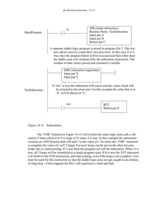
When activated, interrupt routines will stop the PLC, and the ladder logic is inter-
preted immediately. If multiple interrupts occur at the same time the ones with the higher
priority will occur first. If the PLC is in the middle of a program scan when interrupted
this can cause problems. To overcome this a program can disable interrupts temporarily
using the UID and UIE functions. Figure 16.16 shows an example where the interrupts are
disabled for a FAL instruction. Only the ladder logic between the UID and UIE will be
disabled, the first line of ladder logic could be interrupted. This would be important if an
interrupt routine could change a value between n[0] and n[4]. For example, an interrupt
could occur while the FAL instruction was at n[7]=n[2]+5. The interrupt could change
the values of n[1] and n[4], and then end. The FAL instruction would then complete the
calculations. But, the results would be based on the old value for n[1] and the new value
for n[4].](https://image.slidesharecdn.com/plc-programmable-logic-controller-book-230318130132-22ebd54b/85/PLC-Programmable-Logic-Controller-Book-pdf-414-320.jpg)
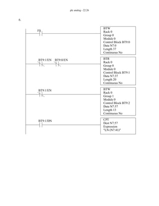
![plc advanced functions - 16.17
Figure 16.16 Disabling Interrupts
16.4 INPUT AND OUTPUT FUNCTIONS
16.4.1 Immediate I/O Instructions
The input scan normally records the inputs before the program scan, and the output
scan normally updates the outputs after the program scan, as shown in Figure 16.17.
Immediate input and output instructions can be used to update some of the inputs or out-
puts during the program scan.
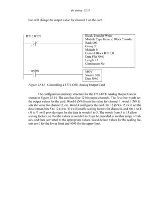
UID
X
A
UIE
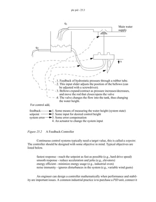
FAL
Control c
length 5
position 0
Mode all
Destination n[5 + c.POS]
Expression n[c.POS] + 5
B](https://image.slidesharecdn.com/plc-programmable-logic-controller-book-230318130132-22ebd54b/85/PLC-Programmable-Logic-Controller-Book-pdf-415-320.jpg)
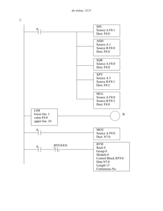
![plc advanced functions - 16.18
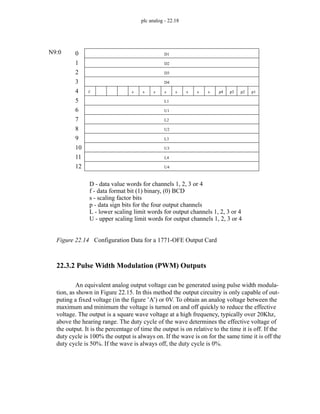
Figure 16.17 Input, Program and Output Scan
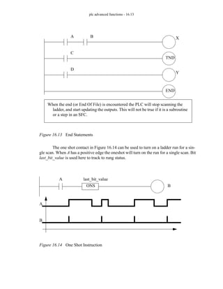
Figure 16.18 shows a segment within a program that will update the input word
input_value, determine a new value for output_value.1, and update the output word
output_value immediately. The process can be repeated many times during the program
scan allowing faster than normal response times. These instructions are less useful on
newer PLCs with networked hardware and software, so Allen Bradley does not support
IIN for newer PLCs such as ControlLogix, even though the IOT is supported.
• The normal operation of the PLC is
fast [input scan]
slow [ladder logic is checked]
fast [outputs updated]
Input values scanned
Outputs are updated in
memory only, as the
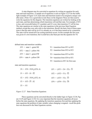
ladder logic is scanned
Output values are
updated to match
values in memory](https://image.slidesharecdn.com/plc-programmable-logic-controller-book-230318130132-22ebd54b/85/PLC-Programmable-Logic-Controller-Book-pdf-416-320.jpg)
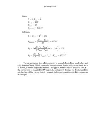
![plc advanced functions - 16.25
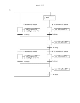
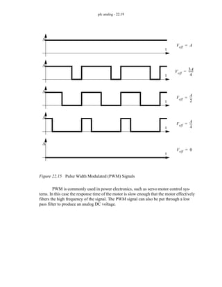
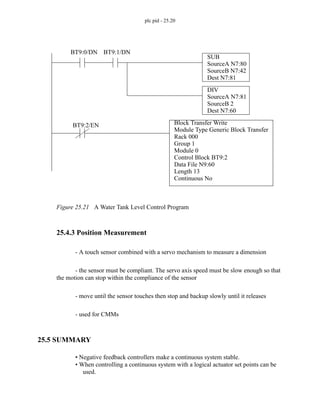
16.6.2 Traffic Light
Problem: Design and write ladder logic for a simple traffic light controller that has
a single fixed sequence of 16 seconds for both green lights and 4 second for both yellow
lights. Use either stacks or sequencers.
Solution: The sequencer is the best solution to this problem.
Figure 16.25 An Example Traffic Light Controller
16.7 SUMMARY
• Shift registers move bits through a queue.
• Stacks will create a variable length list of words.
• Sequencers allow a list of words to be stepped through.
• Parts of programs can be skipped with jump and MCR statements, but MCR
statements shut off outputs.
OUTPUTS
O.0 NSG - north south green
O.1 NSY - north south yellow
O.2 NSR - north south red
O.3 EWG - east west green
O.4 EWY - east west yellow
O.5 EWR - east west red
TON
t
preset 4.0 sec
SQO
File n[0]
mask 0x003F
t.DN
t.DN
Dest. O
Control c
Length 10
Addr.
n[0]
n[1]
n[2]
n[3]
n[4]
n[5]
n[6]
n[7]
n[8]
n[9]
n[10]
Contents (in binary)
0000000000001001
0000000000100001
0000000000100001
0000000000100001
0000000000100001
0000000000100010
0000000000001100
0000000000001100
0000000000001100
0000000000001100
0000000000010100](https://image.slidesharecdn.com/plc-programmable-logic-controller-book-230318130132-22ebd54b/85/PLC-Programmable-Logic-Controller-Book-pdf-423-320.jpg)
![plc advanced functions - 16.27
4. Why are MCR blocks different than JMP statements?
5. What is a suitable reason to use interrupts?
6. When would immediate inputs and outputs be used?
7. Explain the significant differences between shift registers, stacks and sequencers.
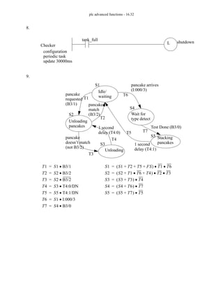
8. Design a ladder logic program that will run once every 30 seconds using interrupts. It will
check to see if a water tank is full with input tank_full. If it is full, then a shutdown value
(’shutdown’) will be latched on.
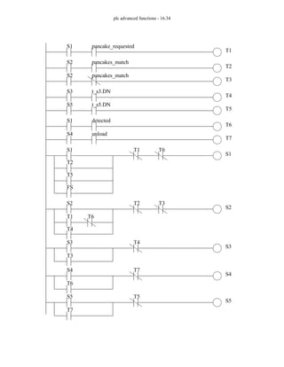
9. At MOdern Manufacturing (MOMs), pancakes are made by multiple machines in three flavors;
chocolate, blueberry and plain. When the pancakes are complete they travel along a single belt,
in no specific order. They are buffered by putting them on the top of a stack. When they arrive
at the stack the input ’detected’ becomes true, and the stack is loaded by making output ’stack’
high for one second. As the pancakes are put on the stack, a color detector is used to determine
the pancakes type. A value is put in ’color_stack’ (1=chocolate, 2=blueberry, 3=plain) and bit
’unload’ is made true. A pancake can be requested by pushing a button (’chocolate’, ’blue-
berry’, ’plain’). Pancakes are then unloaded from the stack, by making ’unload’ high for 1 sec-
ond, until the desired flavor is removed. Any pancakes removed aren’t returned to the stack.
Design a ladder logic program to control this stack.
10. a) What are the two fundamental types of interrupts?
b) What are the advantages of interrupts in control programs?
c) What potential problems can they create?
d) Which instructions can prevent this problem?
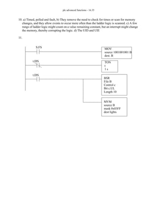
11. Write a ladder logic program to drive a set of flashing lights. In total there are 10 lights con-
nected to ’lights[0]’ to ’lights[9]’. At any time every one out of three lights should be on. Every
second the pattern on the lights should shift towards ’lights[9]’.
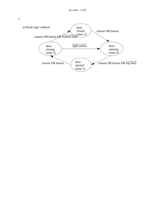
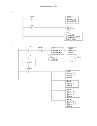
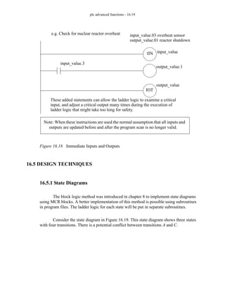
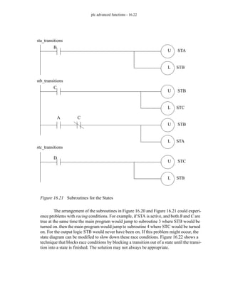
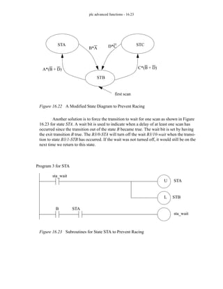
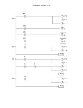
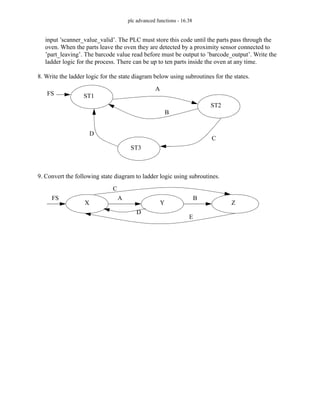
12. Implement the following state diagram using subroutines.
ST0 ST1 ST2
FS
A
B
C D](https://image.slidesharecdn.com/plc-programmable-logic-controller-book-230318130132-22ebd54b/85/PLC-Programmable-Logic-Controller-Book-pdf-425-320.jpg)
![plc advanced functions - 16.28
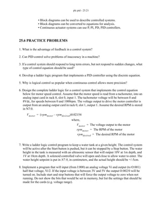
16.9 PRACTICE PROBLEM SOLUTIONS
1.
TON
Timer t
Delay 4s
t.DN
BSR
File b[0]
Control c0
Bit address c0.UL
Length 10
t.DN
BSR
File b[1]
Control c1
Bit address c1.UL
Length 10
BSR
File b[2]
Control c2
Bit address c2.UL
Length 10
BSR
File b[3]
Control c3
Bit address c3.UL
Length 10
BSR
File b[4]
Control c4
Bit address c4.UL
Length 10
BSR
File b[5]
Control c5
Bit address c5.UL
Length 10
b[0] = 0000 0000 0000 1111 (grn EW)
b[1] = 0000 0000 0001 0000 (yel EW)
b[2] = 0000 0011 1110 0000 (red EW)
b[3] = 0000 0011 1100 0000 (grn NS)
b[4] = 0000 0000 0010 0000 (yel NS)
b[5] = 0000 0000 0001 1111 (red NS)](https://image.slidesharecdn.com/plc-programmable-logic-controller-book-230318130132-22ebd54b/85/PLC-Programmable-Logic-Controller-Book-pdf-426-320.jpg)
![plc advanced functions - 16.29
grn_EW
b[0].0
yel_EW
b[1].0
red_EW
b[2].0
grn_NS
b[3].0
yel_NS
b[4].0
red_NS
b[5].0](https://image.slidesharecdn.com/plc-programmable-logic-controller-book-230318130132-22ebd54b/85/PLC-Programmable-Logic-Controller-Book-pdf-427-320.jpg)
![plc advanced functions - 16.30
2.
n[1] = 0000 0000 0000 0110
n[2] = 0000 0000 0001 0000
n[3] = 0000 0000 0001 0000
n[4] = 0000 0000 0000 0100
n[5] = 0000 0000 0000 1000
n[6] = 0000 0000 0100 0000
n[7] = 0000 0000 0110 0000
n[8] = 0000 0000 0000 0001
n[9] = 0000 0000 1000 0000
n[10] = 0000 0000 0000 0100
n[11] = 0000 0000 0000 1100
n[12] = 0000 0000 0000 0000
n[13] = 0000 0000 0100 1000
n[14] = 0000 0000 0000 0010
n[15] = 0000 0000 0000 0100
n[16] = 0000 0000 0000 1000
n[17] = 0000 0000 0000 0001
start
play
play
NEQ
Source A c.POS
Source B 17
TON
Timer t
Delay 4s
t.DN
stop
t.DN
n[0] = 0000 0000 0000 0000
SQO
File n[0]
Mask 0x00FF
Destination lights
Control c
Length 17
Position 0](https://image.slidesharecdn.com/plc-programmable-logic-controller-book-230318130132-22ebd54b/85/PLC-Programmable-Logic-Controller-Book-pdf-428-320.jpg)
![plc advanced functions - 16.31
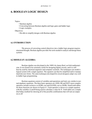
3.
4. In MCR blocks the outputs will all be forced off. This is not a problem for outputs such as
retentive timers and latches, but it will force off normal outputs. JMP statements will skip over
logic and not examine it or force it off.
5. Timed interrupts are useful for processes that must happen at regular time intervals. Polled
interrupts are useful to monitor inputs that must be checked more frequently than the ladder
scan time will permit. Fault interrupts are important for processes where the complete failure
of the PLC could be dangerous.
6. These can be used to update inputs and outputs more frequently than the normal scan time per-
mits.
7. The main differences are: Shift registers focus on bits, stacks and sequencers on words Shift
registers and sequencers are fixed length, stacks are variable lengths
BSR
File b[0]
Control c0
Bit address sensors.0
Length 4
sensors.3
BSR
File b[1]
Control c1
Bit address sensors.1
Length 4
assume:
sensors.0 = left orientation
sensors.1 = right orientation
sensors.2 = reject
b[0].2
left
b[1].1
right
sensors.3 = part sensor
BSR
File b[2]
Control c2
Bit address sensors.2
Length 4
b[2].0
reject](https://image.slidesharecdn.com/plc-programmable-logic-controller-book-230318130132-22ebd54b/85/PLC-Programmable-Logic-Controller-Book-pdf-429-320.jpg)
![plc advanced functions - 16.33
TON
timer t_s3
delay 1s
TON
timer t_s5
delay 1s
S3
S5
B3/0
S2
O:001/0
stack
LFL
source color_detect
LIFO n[0]
Control c
length 10
position 0
LFU
LIFO n[0]
destination waiting_color
Control c
length 10
position 0
EQU
SourceA waiting_color
SourceB req_color
pancakes_match
chocolate
pancake_requested
blueberry
plain
chocolate MOV
Source 1
Dest req_color
blueberry MOV
Source 2
Dest req_color
plain MOV
Source 3
Dest req_color](https://image.slidesharecdn.com/plc-programmable-logic-controller-book-230318130132-22ebd54b/85/PLC-Programmable-Logic-Controller-Book-pdf-431-320.jpg)
![plc advanced functions - 16.37
16.10 ASSIGNMENT PROBLEMS
1. Using 3 different methods write a program that will continuously cycle a pattern of 12 lights
connected to a PLC output card. The pattern should have one out of every three lights set. The
light patterns should appear to move endlessly in one direction.
2. Look at the manuals for the status memory in your PLC.
a) Describe how to run program ’GetBetter’ when a divide by zero error occurs.
b) Write the ladder logic needed to clear a PLC fault.
c) Describe how to set up a timed interrupt to run ’Slowly’ every 2 seconds.
3. Write an interrupt driven program that will run once every 5 seconds and calculate the average
of the numbers from ’f[0]’ to ’f[19]’, and store the result in ’f_avg’. It will also determine the
median and store it in ’f_med’.
4. Write a program for SPC (Statistical Process Control) that will run once every 20 minutes using
timed interrupts. When the program runs it will calculate the average of the data values in
memory locations ’f[0]’ to ’f[39]’ (Note: these values are written into the PLC memory by
another PLC using networking). The program will also find the range of the values by subtract-
ing the maximum from the minimum value. The average will be compared to upper (f_ucl_x)
and lower (f_lcl_x) limits. The range will also be compared to upper (f_ucl_r) and lower
(f_lcl_r) limits. If the average, or range values are outside the limits, the process will stop, and
an ‘out of control’ light will be turned on. The process will use start and stop buttons, and
when running it will set memory bit ’in_control’.
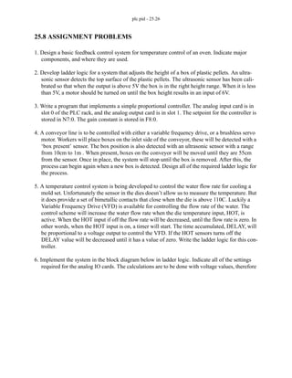
5. Develop a ladder logic program to control a light display outside a theater. The display consists
of a row of 8 lights. When a patron walks past an optical sensor the lights will turn on in
sequence, moving in the same direction. Initially all lights are off. Once triggered the lights
turn on sequentially until all eight lights are on 1.6 seconds latter. After a delay of another 0.4
seconds the lights start to turn off until all are off, again moving in the same direction as the
patron. The effect is a moving light pattern that follows the patron as they walk into the theater.
6. Write the ladder logic diagram that would be required to execute the following data manipula-
tion for a preventative maintenance program.
i) Keep track of the number of times a motor was started with toggle switch #1.
ii) After 2000 motor starts turn on an indicator light on the operator panel.
iii) Provide the capability to change the number of motor starts being tracked, prior
to triggering of the indicator light. HINT: This capability will only require the
change of a value in a compare statement rather than the addition of new lines
of logic.
iv) Keep track of the number of minutes that the motor has run.
v) After 9000 minutes of operation turn the motor off automatically and also turn
on an indicator light on the operator panel.
7. Parts arrive at an oven on a conveyor belt and pass a barcode scanner. When the barcode scan-
ner reads a valid barcode it outputs the numeric code as 32 bits to ’scanner_value’ and sets](https://image.slidesharecdn.com/plc-programmable-logic-controller-book-230318130132-22ebd54b/85/PLC-Programmable-Logic-Controller-Book-pdf-435-320.jpg)
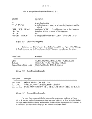
![plc st - 19.5
Figure 19.5 Variable Declaration Examples
Basic numbers are shown in Figure 19.6. Note the underline ‘_’ can be ignored, it
can be used to break up long numbers, ie. 10_000 = 10000. These are the literal values dis-
cussed for Ladder Logic.
Figure 19.6 Literal Number Examples
Text Program Line
VAR AT %B3:0 : WORD; END_VAR
VAR AT %N7:0 : INT; END_VAR
VAR RETAIN AT %O:000 : WORD ; END_VAR
VAR_GLOBAL A AT %I:000/00 : BOOL ; END_VAR
VAR_GLOBAL A AT %N7:0 : INT ; END_VAR
VAR A AT %F8:0 : ARRAY [0..14] OF REAL; END_VAR
VAR A : BOOL; END_VAR
VAR A, B, C : INT ; END_VAR
VAR A : STRING[10] ; END_VAR
VAR A : ARRAY[1..5,1..6,1..7] OF INT; END_VAR
VAR RETAIN RTBT A : ARRAY[1..5,1..6] OF INT;
END_VAR
VAR A : B; END_VAR
VAR CONSTANT A : REAL := 5.12345 ; END_VAR
VAR A AT %N7:0 : INT := 55; END_VAR
VAR A : ARRAY[1..5] OF INT := [5(3)]; END_VAR
VAR A : STRING[10] := ‘test’; END_VAR
VAR A : ARRAY[0..2] OF BOOL := [1,0,1]; END_VAR
VAR A : ARRAY[0..1,1..5] OF INT := [5(1),5(2)];
END_VAR
Description
a word in bit memory
an integer in integer memory
makes output bits retentive
variable ‘A’ as input bit
variable ‘A’ as an integer
an array ‘A’ of 15 real values
a boolean variable ‘A’
integers variables ‘A’, ‘B’, ‘C’
a string ‘A’ of length 10
a 5x6x7 array ‘A’ of integers
a 5x6 array of integers, filled
with zeros after power off
‘A’ is data type ‘B’
a constant value ‘A’
‘A’ starts with 55
‘A’ starts with 3 in all 5 spots
‘A’ contains ‘test’ initially
an array of bits
an array of integers filled with 1
for [0,x] and 2 for [1,x]
number type
integers
real numbers
real with exponents
binary numbers
octal numbers
hexadecimal numbers
boolean
examples
-100, 0, 100, 10_000
-100.0, 0.0, 100.0, 10_000.0
-1.0E-2, -1.0e-2, 0.0e0, 1.0E2
2#111111111, 2#1111_1111, 2#1111_1101_0110_0101
8#123, 8#777, 8#14
16#FF, 16#ff, 16#9a, 16#01
0, FALSE, 1, TRUE](https://image.slidesharecdn.com/plc-programmable-logic-controller-book-230318130132-22ebd54b/85/PLC-Programmable-Logic-Controller-Book-pdf-456-320.jpg)
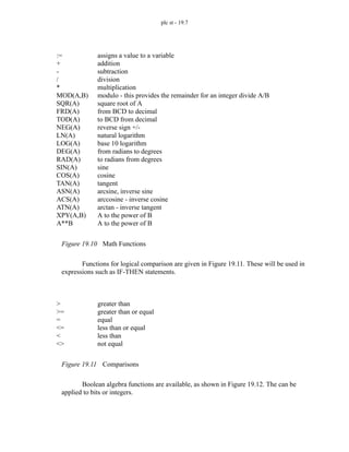
![plc st - 19.9
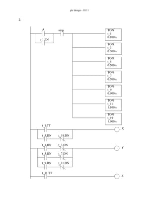
Special instructions include those shown in Figure 19.15.
Figure 19.15 Special Instructions
19.2.2 Putting Things Together in a Program
Consider the program in Figure 19.16 to find the average of five values in a real
array ’f[]’. The FOR loop in the example will loop five times adding the array values.
After that the sum is divided to get the average.
Figure 19.16 A Program To Average Five Values In Memory With A For-Loop
The previous example is implemented with a WHILE loop in Figure 19.17. The
main differences is that the initial value and update for ’i’ must be done manually.
Figure 19.17 A Program To Average Five Values In Memory With A While-Loop
RETAIN();
IIN();
EXIT;
EMPTY
causes a bit to be retentive
immediate input update
will quit a FOR or WHILE loop
avg := 0;
FOR (i := 0 TO 4) DO
avg := avg + f[i];
END_FOR;
avg := avg / 5;
avg := 0;
i := 0;
WHILE (i < 5) DO
avg := avg + f[i];
i := i + 1;
END_WHILE;
avg := avg / 5;](https://image.slidesharecdn.com/plc-programmable-logic-controller-book-230318130132-22ebd54b/85/PLC-Programmable-Logic-Controller-Book-pdf-460-320.jpg)


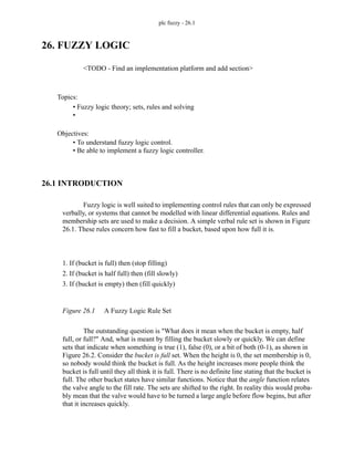
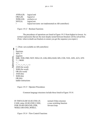
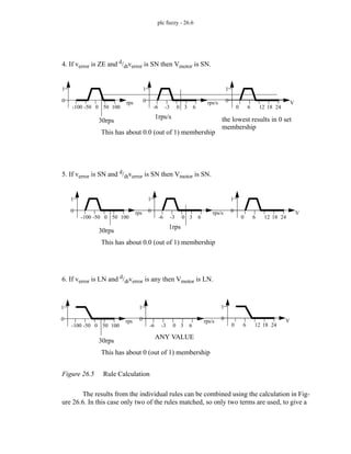
![plc fuzzy - 26.3
Figure 26.3 Fuzzy Rule Solving
An example of a fuzzy logic controller for controlling a servomotor is shown in
Figure 26.4 [Lee and Lau, 1988]. This controller rules examines the system error, and the
rate of error change to select a motor voltage. In this example the set memberships are
defined with straight lines, but this will have a minimal effect on the controller perfor-
mance.
height angle
1
0
1
0
1
0
1
0
1
0
1
0
stop filling
fill slowly
fill quickly
bucket is full
bucket is half full
bucket is empty
angle
1. If (bucket is full) then (stop filling)
2. If (bucket is half full) then (fill slowly)
3. If (bucket is empty) then (fill quickly)
angle
height
height
a1
a2](https://image.slidesharecdn.com/plc-programmable-logic-controller-book-230318130132-22ebd54b/85/PLC-Programmable-Logic-Controller-Book-pdf-625-320.jpg)
![plc software - 32.12
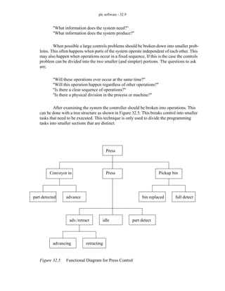
2. A basic model of the system is developed in terms of the inputs and outputs.
This might include items such as when sensor changes are expected, what
effects actuators should have, and expected operator inputs.
3. A system simulator is constructed with some combination of specialized soft-
ware and hardware.
4. The system is verified for the expect operation of the system.
5. The system is then used for testing software and verifying the operation.
A detailed description of simulator usage is available [Kinner, 1992].
32.5 DOCUMENTATION
Poor documentation is a common complaint lodged against control system design-
ers. Good documentation is developed as a project progresses. Many engineers will leave
the documentation to the end of a project as an afterthought. But, by that point many of the
details have been forgotten. So, it takes longer to recall the details of the work, and the
report is always lacking.
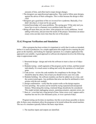
A set of PLC design forms are given in Figure 32.6 to Figure 32.12. These can be
used before, during and after a controls project. These forms can then be kept in design or
maintenance offices so that others can get easy access and make updates at the controller
is changed. Figure 32.6 shows a design cover page. This should be completed with infor-
mation such as a unique project name, contact person, and controller type. The list of
changes below help to track design, redesign and maintenance that has been done to the
machine. This cover sheet acts as a quick overview on the history of the machine. Figure
32.7 to Figure 32.9 show sheets that allow free form planning of the design. Figure 32.10
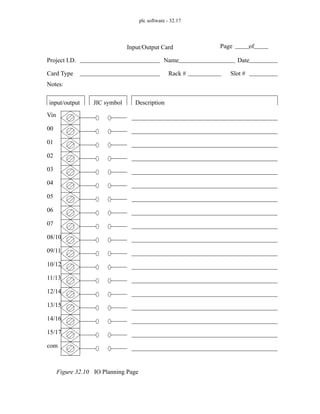
shows a sheet for planning the input and output memory locations. Figure 32.11 shows a
sheet for planning internal memory locations, and finally Figure 32.12 shows a sheet for
planning the ladder logic. The sheets should be used in the order they are given, but they
do not all need to be used. When the system has been built and tested, a copy of the work-
ing ladder logic should be attached to the end of the bundle of pages.](https://image.slidesharecdn.com/plc-programmable-logic-controller-book-230318130132-22ebd54b/85/PLC-Programmable-Logic-Controller-Book-pdf-727-320.jpg)
![plc software - 32.22
ures to the total failures.
- To calculate the SFF
- do an FMEA for each system component in the system
- classify failure modes as safe or dangerous
- calculate the probabilities of safe/dangerous failures (S/D [0, 1])
- estimate the fraction of the failures that can be detected (F [0, 1])
- SFF = ....
-
32.8 LEAN MANUFACTURING
- lean manufacturing has received attention lately, but it embodies many common
sense machine design concepts.
- In simple terms lean manufacturing involves eliminating waste from a system.
- Some general concepts to use when designing lean machines include,
- setups should be minimized or eliminated
- product changeovers should be minimized or eliminated
- make the tool fit the job, not the other way. If necessary, design a new tool
- design the machine be faster than the needed cycle time to allow flexibil-
ity and excess capacity - this does seem contradictory, but it allows better
use of other resources. For example, if a worker takes a bathroom break,
the production can continue with fewer workers.
- allow batches with a minimum capacity of one.
- people are part of the process and should integrate smoothly - the motions
or workers are often described as dance like.
- eliminate wasted steps, all should go into making the part
- work should flow smoothly to avoid wasted motion
- do not waste motion by spacing out machines
- make-one, check-one
- design "decouplers" to allow operations to happen independantly.
- eliminate material waste that does not go into the product
- pull work through the cell](https://image.slidesharecdn.com/plc-programmable-logic-controller-book-230318130132-22ebd54b/85/PLC-Programmable-Logic-Controller-Book-pdf-737-320.jpg)

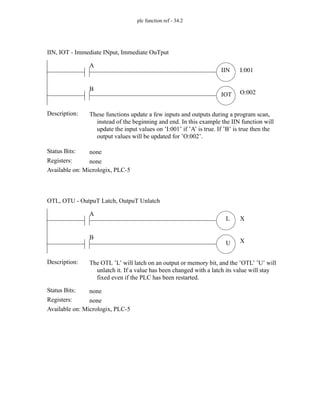
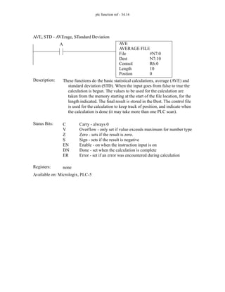
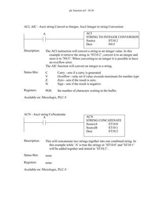
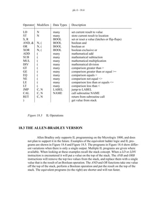
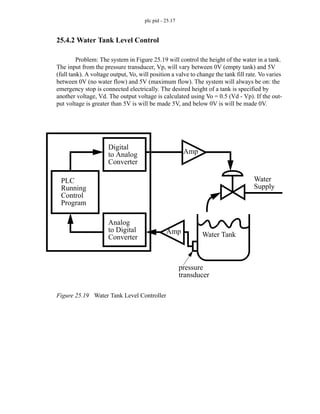
![plc function ref - 34.42
34.2 DATA TYPES
The following table describes the arguments and return values for functions. Some
notes are;
• ’immediate’ values are numerical, not memory addresses.
• ’returns’ indicates that the function returns that data value.
• numbers between ’[’ and ’]’ indicate a range of values.
• values such as ’yes’ and ’no’ are typed in literally.
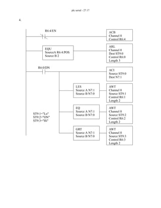
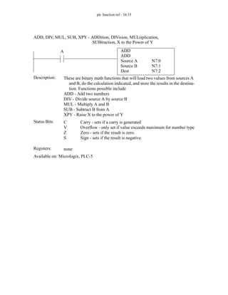
AWT
ASCII WRITE
Channel
Source
Control
0
ST11:9
A
Status Bits:
The AWT instruction will send a character string. In this example, when
’A’ goes from false to true, up to 14 characters will be sent from
’ST11:9’ to channel 0. This does not append any end of line charac-
ters.
The AWA function has a similar operation, except that the channel con-
figuration characters are added - by default these are ’CR’ and ’LF’.
Description:
EN
DN
ER
UL
EM
EU
enable - this will be set while the instruction is active
done - this will be set after the string has been sent
error bit - set when an error has occurred
unload -
empty - set if no string was found
queue -
Registers: POS the number of characters sent instructions
Available on: Micrologix, PLC-5
AWT, AWA - Ascii WriTe, Ascii Write Append
String Length
Characters Sent
R6:3
14](https://image.slidesharecdn.com/plc-programmable-logic-controller-book-230318130132-22ebd54b/85/PLC-Programmable-Logic-Controller-Book-pdf-791-320.jpg)
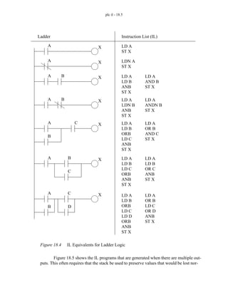
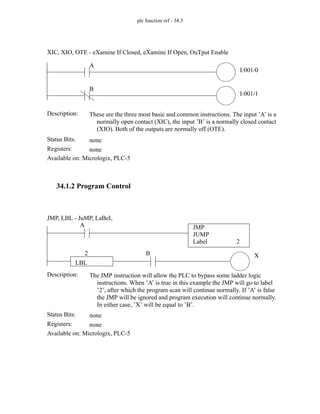
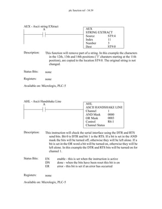
![plc function ref - 34.43
Table 1: Instruction Data Types
Function Argument Data Types Edge Triggered
ABL channel
control
characters
immediate int [0-4]
R
returns N
yes
ACB channel
control
characters
immediate int [0-4]
R
returns N
yes
ACI source
destination
ST
N
no
ACN source A
source B
ST
ST
no
ACS source
destination
N,F,immediate
N,F
no
ADD source A
source B
destination
N,F,immediate
N,F,immediate
N,F
no
AEX source
index
number
destination
ST
immediate int [0-82]
immediate int [0-82]
ST
no
AFI no
AHL channel
AND mask
OR mask
control
immediate int [0-4]
immediate hex [0000-ffff]
immediate hex [0000-ffff]
R
yes
AIC source
destination
N, immediate int
ST
no
ARD channel
destination
control
string length
characters read
immediate int [0-4]
ST
R
immediate int [0-83]
returns N
yes](https://image.slidesharecdn.com/plc-programmable-logic-controller-book-230318130132-22ebd54b/85/PLC-Programmable-Logic-Controller-Book-pdf-792-320.jpg)
![plc function ref - 34.44
ARL channel
destination
control
string length
characters read
immediate int [0-4]
ST
R
immediate int [0-83]
returns N
yes
ASC source
index
search
result
ST
N, immediate
ST
R
no
ASN source
destination
N,F,immediate
N,F
no
ASR source A
source B
ST
ST
no
ATN source
destination
N,F,immediate
N,F
no
AVE file
destination
control
length
position
#F,#N
F,N
R
N,immediate int
returns N
yes
AWA channel
source
control
string length
characters sent
immediate int [0-4]
ST
R
immediate int [0-82]
returns N
yes
AWT channel
source
control
length
characters sent
N, immediate int
ST
R
immediate int [0-82]
returns N
yes
BSL file
control
bit address
length
#B,#N
R
any bit
immediate int [0-16000]
yes
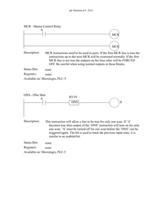
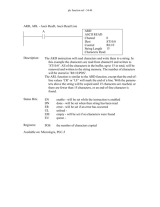
Table 1: Instruction Data Types
Function Argument Data Types Edge Triggered](https://image.slidesharecdn.com/plc-programmable-logic-controller-book-230318130132-22ebd54b/85/PLC-Programmable-Logic-Controller-Book-pdf-793-320.jpg)
![plc function ref - 34.45
BSR file
control
bit address
length
#B,#N
R
any bit
immediate int [0-16000]
yes
BTD source
source bit
destination
destination bit
length
N,B,immediate
N,immediate int [0-15]
N
immediate int [0-15]
immediate int [0-15]
no
BTR rack
group
module
control block
data file
length
continuous
immediate octal [000-277]
immediate octal [0-7]
immediate octal [0-1]
BT,N
N
immediate int [0-64]
’yes’,’no’
yes
BTW rack
group
module
control block
data file
length
continuous
immediate octal [000-277]
immediate octal [0-7]
immediate octal [0-1]
BT,N
N
immediate int [0-64]
’yes’,’no’
yes
CLR destination N,F no
CMP expression expression no
COP source
destination
length
#any
#any
immediate int [0-1000]
no
COS source
destination
F,immediate
F
no
CPT destination
expression
N,F
expression
no
CTD counter
preset
accumulated
C
returns N
returns N
yes
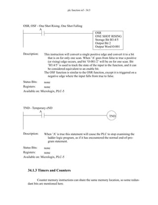
Table 1: Instruction Data Types
Function Argument Data Types Edge Triggered](https://image.slidesharecdn.com/plc-programmable-logic-controller-book-230318130132-22ebd54b/85/PLC-Programmable-Logic-Controller-Book-pdf-794-320.jpg)


![PLC Ladder Programming [Mechatronics]](https://cdn.slidesharecdn.com/ss_thumbnails/plc-ppt-snteli-200503070616-thumbnail.jpg?width=640&height=640&fit=bounds)