Downloaded 17 times
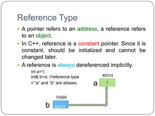
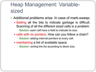
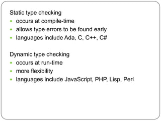
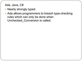
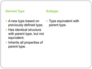
![Array Types
Homogeneous
Reference – aggregate name & subscript
e.g. arrayName [10]
Element type & Subscript type
Subscript range checking
Subscript lower binding](https://image.slidesharecdn.com/plc1-111208104143-phpapp01/85/Plc-1-8-320.jpg)
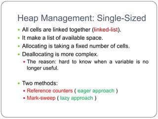
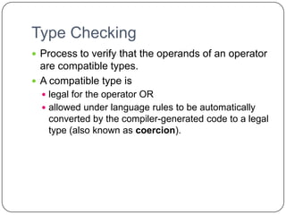
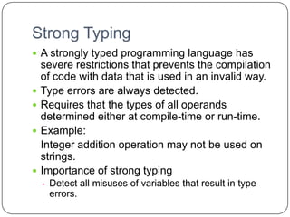
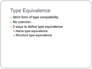
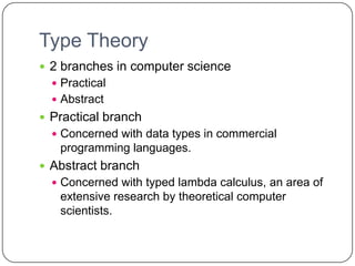
![Arrays and Indices
Ada :
e.g. name (10) : Array? Element?
Ordinal Type subscript : e.g. day(Monday)
Perl
Sign @ for array : e.g. @list
Sign $ for scalars : e.g.$list[1]
Negative subscript
+ve subscript 0 1 2 3 4
Array’s 0 1 2 3 4
Element
-ve subscript -5 -4 -3 -2 -1](https://image.slidesharecdn.com/plc1-111208104143-phpapp01/85/Plc-1-9-320.jpg)
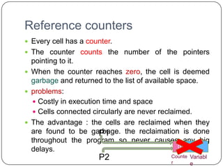
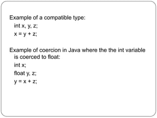
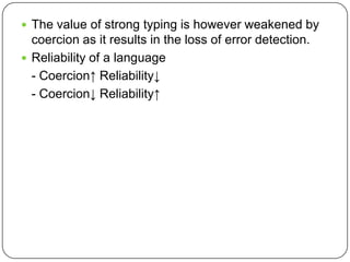
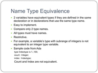
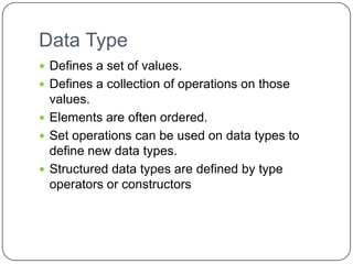
![Array Initialization
Languag Example
e
Fortran Integer, Dimension(3) :: List = (/0, 5, 5/)
95
C int list [ ] = {4, 5, 6, 83};
C, C++ char name [ ] = “freddie”;
char *name [ ] = (“Bob”, “Jake”, “Darcie”); //pointer
Java String[ ] names = [“Bob”, “Jake”, Darcie”];
Ada List : array (1..5) of Integer := (1, 3, 4, 7, 8);
Bunch : array (1..5) of Integer := (1 => 17, 3 => 34, others =>
List Comprehensions of Python
0);
Syntax : [expression for iterate_var in array if condition ]
Example :[x*x for x in range (12) if x %
3 == 0 ]
[0, 1, 2, 3, 4, 5, 6, 7, 8, 9, 10, 11,
12] [0, 9, 36, 81,
[0, 3, 6, 9, 144]](https://image.slidesharecdn.com/plc1-111208104143-phpapp01/85/Plc-1-11-320.jpg)
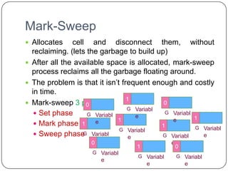
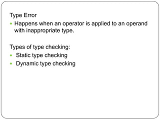
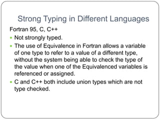
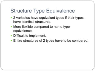
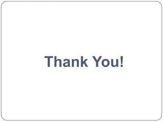
![Rectangular & Jagged Array
Rectangular Array Jagged Array
Fortran, Ada, C# C, C++, Java, C#
myArray [3, 7] myArray [3] [7]](https://image.slidesharecdn.com/plc1-111208104143-phpapp01/85/Plc-1-13-320.jpg)
![6.5.7 Slices
Python: mat 0 1 2
0 1 2 3
1 4 5 6
2 7 8 9
mat [1] -> [4, 5, 6]
mat [0] [0 : 2] -> [1 ,2]
vecto 0 1 2 3 4 5 6 7 8
r
0 2 4 6 8 10 12 14 16 17
vector [0 : 8 : 2] -> [2 ,6, 10,
14]](https://image.slidesharecdn.com/plc1-111208104143-phpapp01/85/Plc-1-14-320.jpg)
![6.5.9 Implementation of Array Types
Array : 3 4 7 Row Major Order Column Major Order
3 4 7 34 7
6 2 5 6 2 5 6 2 5
1 3 8 1 3 8 1 3 8
3, 4, 7, 6, 2, 5, 1, 3, 8 3, 6, 1, 4, 2, 3, 7, 5, 8
location(a [i, j]) = a 1 2 3 4 5 6 7 8 9
adress of a[1, 1] + (( 1
((# of rows above ith row) 2
3
* (size of row)) + 4
(# of columns left jth column))
5 X
* element size) 6
location (a [5, 6]) Adress of a[1, 1] + 4 9 + 5 ) x element
= (( x size)](https://image.slidesharecdn.com/plc1-111208104143-phpapp01/85/Plc-1-15-320.jpg)
![Associative Arrays
An unordered collection of data elements that
are indexed by an equal number of values called
keys.
Each element is a pair of entities (key , value)
Key Value
Eujinn 70
Marry 99 => Dataset[“Eujinn”] = 70;
Joanne 55 => Dataset[“Marry”] = 99;
Johnny 41 => Dataset[“Joanne”] = 55;
=> Dataset[“Johnny”] = 41;](https://image.slidesharecdn.com/plc1-111208104143-phpapp01/85/Plc-1-16-320.jpg)
![Associative Array : Operation
Assignments
$salaries{“Perry”} = 58850; //In Perl
salaries[“Perry”] = 58850; //In C++
Delete
delete $salaries{“Gary”}; //In Perl
salaries.erase(“Gary”); //In C++
Exists
If(exists $salaries{“Shelly”}) … //In Perl
If( salaries.find(“Shelly”)) //In C++](https://image.slidesharecdn.com/plc1-111208104143-phpapp01/85/Plc-1-18-320.jpg)
![Union Type : Implementation
Implemented by using the same address for
every variant
Storage is allocated to largest variant
1110100 0000001 0000000 0000000
0 1 0 0
C[0] => 232 C[1] = 3
a => 100010 (11111010002)
*32 bits is allocated becaus
int has larger size](https://image.slidesharecdn.com/plc1-111208104143-phpapp01/85/Plc-1-24-320.jpg)
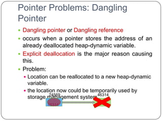

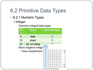
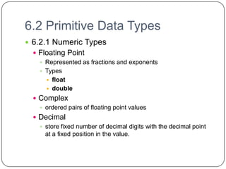
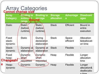
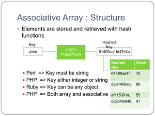
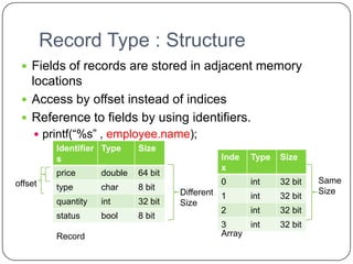
The document discusses various primitive data types including numeric, boolean, character, and string types. It describes integer types like byte, short, int that can store negative numbers using two's complement. Floating point types are represented as fractions and exponents. Boolean types are either true or false. Character types are stored as numeric codes. String types can have static, limited dynamic, or fully dynamic lengths. User-defined types like enumerations and subranges are also covered. The document also discusses array types including their initialization, operations, and implementation using row-major and column-major ordering. Associative arrays are described as unordered collections indexed by keys. Record and union types are summarized.