The document discusses various primitive data types including numeric, boolean, character, and string types. It describes integers, floating point numbers, complex numbers, decimals, booleans, characters, and strings. It also covers array types like static, dynamic, and associative arrays. Other topics include records, slices, and unions.

1. Data Types
Ng Eu Jinn 1071112650
Tan Chin Tong 1081106274
Ng Cong Jie 1071117296
Mostafa Abedi 1091108989
Tan Joanne 1071115484

2. 6.2 Primitive Data Types
 6.2.1 Numeric Types
 Integer
 Common integral data types
Bit Name Decimal Digits
8 byte 3
16 short 5
32 int and long 10
 Store negative integers
 Twos complement

3. 6.2 Primitive Data Types
 6.2.1 Numeric Types
 Floating Point
 Represented as fractions and exponents
 Types
 float
 double
 Complex
 ordered pairs of floating point values
 Decimal
 store fixed number of decimal digits with the decimal point at a fixed
position in the value.

4. 6.2 Primitive Data Types
 6.2.2 Boolean Types
 true or false
 represented by a single bit(can’t access efficiently)
 stored in the smallest efficiently addressable cell of memory
(1 byte)
 6.2.3 Character Types
 stored as numeric codings (computer)
 ASCII > UCSS-2 >UCS-4

5. 6.3 Character String Types
 String operations
 Assignment &Comparison
 complicated(string operands of different lengths)
 Catenation
 Substring reference(slices)
 reference to a substring of a given string
 Pattern matching
 supported directly in the language or provided library

6. 6.3 Character String Types
 String Length Options
 Static length strings
 Limited dynamic length strings
 varying length up to a declared and fixed maximum set by the variable’s
definition
 store any number of character between 0 and maximum
 Dynamic length strings
 varying length with no maximum
 overhead of dynamic storage allocation and deallocation (maximum
flexibility)

7. 6.4 User-Defined Ordinal Types
 range of possible value can be associated with the set of
positive integers
 Enumeration
 all of the possible values which are named constants are provided in the
definition
 Sub range
 contiguous subsequence of an ordinal type

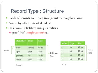
8. Array Types
 Homogeneous
 Reference – aggregate name & subscript
e.g. arrayName [10]
 Element type & Subscript type
 Subscript range checking
 Subscript lower binding

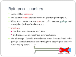
9. Arrays and Indices
 Ada :
 e.g. name (10) : Array? Element?
 Ordinal Type subscript : e.g. day(Monday)
 Perl
 Sign @ for array : e.g. @list
 Sign $ for scalars : e.g.$list[1]
 Negative subscript
+ve subscript 0 1 2 3 4
Array’s Element 0 1 2 3 4
-ve subscript -5 -4 -3 -2 -1

10. Array Categories
Cannot change size
Array Binding to Binding to Storage Advantages Disadvanta
Category subscript storage allocation ges
range Bound
Static Static Static Stack Efficient Bound in
(before (before entire
runtime) runtime) execution
Fixed stack- Static During Stack Space efficient Allocation
dynamic declaration &deallocation
elaboration time
Stack- Dynamic at Dynamic at Stack Flexible -
dynamic elaboration elaboration
Fixed heap- Dynamic Dynamic Heap Flexible Longer
dynamic when when allocation
Changeable requested requested time
Heap- Dynamic Dynamic Heap Flexible Longer
dynamic allocation&de
allocation

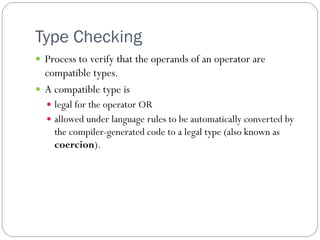
11. Array Initialization
Language Example
Fortran 95 Integer, Dimension(3) :: List = (/0, 5, 5/)
C int list [ ] = {4, 5, 6, 83};
C, C++ char name [ ] = “freddie”;
char *name [ ] = (“Bob”, “Jake”, “Darcie”); //pointer
Java String[ ] names = [“Bob”, “Jake”, Darcie”];
Ada List : array (1..5) of Integer := (1, 3, 4, 7, 8);
Bunch : array (1..5) of Integer := (1 => 17, 3 => 34, others => 0);
List Comprehensions of Python
Syntax : [expression for iterate_var in array if condition ]
Example : [ x * x for x in range (12) if x % 3 == 0 ]
[0, 1, 2, 3, 4, 5, 6, 7, 8, 9, 10, 11, 12]
[0, 9, 36, 81, 144]
[0, 3, 6, 9, 12]

12. Array Operations
 C -> through Java, C++ and C#
 Perl -> Array assignments, comparisons
 Ada -> Array assignments, catenation, equality and inequality
operators
 Python -> Array catenation, membership, comparisons
 Tuples : immutable and use parentheses
 Fortran 95 -> Elemental operations
 Array-Processing Language (APL)

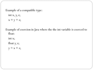
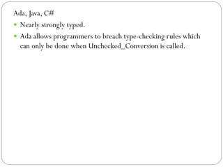
13. Rectangular & Jagged Array
Rectangular Array Jagged Array
Fortran, Ada, C# C, C++, Java, C#
myArray [3, 7] myArray [3] [7]

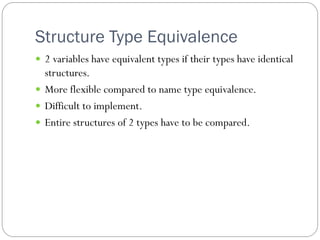
14. 6.5.7 Slices
Python: mat 0 1 2
0 1 2 3
1 4 5 6
2 7 8 9
mat [1] -> [4, 5, 6]
mat [0] [0 : 2] -> [1 ,2]
vector 0 1 2 3 4 5 6 7 8
0 2 4 6 8 10 12 14 16 17
vector [0 : 8 : 2] -> [2 ,6, 10, 14]

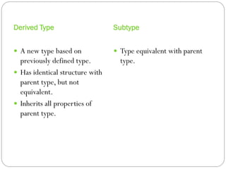
15. 6.5.9 Implementation of Array Types
 Array : 3 4 7 Row Major Order Column Major Order
3 4 7 34 7
6 2 5 6 2 5 6 2 5
1 3 8 1 3 8 1 3 8
3, 4, 7, 6, 2, 5, 1, 3, 8 3, 6, 1, 4, 2, 3, 7, 5, 8
 location(a [i, j]) = a 1 2 3 4 5 6 7 8 9
adress of a[1, 1] + (( 1
2
((# of rows above ith row)
3
* (size of row)) + 4
(# of columns left jth column)) 5 X
* element size) 6
location (a [5, 6]) = Adress of a[1, 1] + ( ( 4 x 9 + 5 ) x element size)

16. Associative Arrays
 An unordered collection of data elements that are indexed
by an equal number of values called keys.
 Each element is a pair of entities (key , value)
Key Value
Eujinn 70 => Dataset[“Eujinn”] = 70;
Marry 99 => Dataset[“Marry”] = 99;
Joanne 55 => Dataset[“Joanne”] = 55;
=> Dataset[“Johnny”] = 41;
Johnny 41

17. Associative Array : Structure
 Elements are stored and retrieved with hash functions
Key Hashed Key
John HASH 61409aa1fd47d4a
FUNCTION
Hashed Key Value
 Perl => Key must be string
61409aa1f… 70
 PHP => Key either integer or string
8a31409aa.. 99
 Ruby => Key can be any object af115391a.. 55
 PHP => Both array and associative array cc2d4fe946.. 41

18. Associative Array : Operation
 Assignments
 $salaries{“Perry”} = 58850; //In Perl
 salaries[“Perry”] = 58850; //In C++
 Delete
 delete $salaries{“Gary”}; //In Perl
 salaries.erase(“Gary”); //In C++
 Exists
 If(exists $salaries{“Shelly”}) … //In Perl
 If( salaries.find(“Shelly”)) //In C++

19. Record Type
 Is used to group collection of data with different
(heterogeneous) data-type.
 Eg: Struct in C, C++ and C#
struct Employee
{
string name;
int age;
float salary;
};

20. Record Type : Structure
 Fields of records are stored in adjacent memory locations
 Access by offset instead of indices
 Reference to fields by using identifiers.
 printf(“%s” , employee.name);
Identifier Type Size
s Index Type Size
price double 64 bit 0 int 32 bit
offset Same
type char 8 bit 1 int 32 bit
Different Size
quantity int 32 bit Size 2 int 32 bit
status bool 8 bit 3 int 32 bit
Record Array

21. Record Type: Operations
 Initialization
 Aggregate literals
 Employee e = {“John”, 28, 3000.0f};
 Assignments
 Comparison
 MOVE CORRESPONDING
 In COBOL, copies all the field from source record to the destination
field record with the same name.
 MOVE CORRESPONDING INPUT-RECORD TO OUTPUT-
RECORD

22. Union Type
 A type whose variable may store different type values at
different times during program execution
 Specifying Union
 In C / C++ => union
 In Fortran => Equivalence

23. Union Type : Design Issue
 Type Checking one of the major design issue
 2 ways of implementations
 Free Union
 Programmers are allowed complete freedom from type checking in their
use
 Use in C, C++, Fortran
 Discriminated Union
 Type indicator(tag) is used for type checking
 Use in ALGOL 68 , ADA

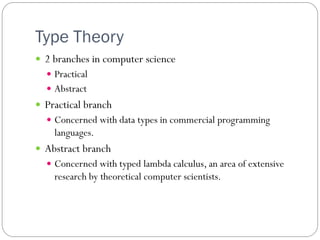
24. Union Type : Implementation
 Implemented by using the same address for every variant
 Storage is allocated to largest variant
11101000 00000011 00000000 00000000
C[0] => 232 C[1] = 3
a => 100010 (11111010002)
*32 bits is allocated because
int has larger size

25. Pointer Problems: Dangling Pointer
 Dangling pointer or Dangling reference
 occurs when a pointer stores the address of an already
deallocated heap-dynamic variable.
 Explicit deallocation is the major reason causing this.
 Problem:
 Location can be reallocated to a new heap-dynamic variable.
 the location now could be temporarily used by storage
management system.
74569 46314
46314

26. Solution: Tombstone
 Tombstones:
 Every heap-dynamic variable includes an extra cell called
tombstone
 The Tombstone is a pointer to the heap dynamic variable.
 When the heap-dynamic variable is deallocated, the tombstone
is set to NULL.
 Disadvantages :
 Costly in memory and time.
74569 65742 46314
65742 NULL
46314
Pointer Tombstone Heap-dynamic Variable

27. Solution: Lock-and-Keys
 Pointers instead of only being an address, also have a key and are made
into a pair. (key, address)
 Heap-dynamic variables also have a header containing a lock.
 When allocated, the keya and the lock are set the same. (key=lock)
 Access is granted only if the lock and key match. Otherwise it’s an error.
 In deallocating, the lock is cleared to an illegal lock value. When other
pointers try to access it, the key doesn’t match the lock hence it is not
allowed.
Pointer
12 54
12
KEY address LOCK Heap-dynamic variable

28. Lost Heap-Dynamic Variables
 An allocated heap-dynamic variable that is not accessible
anymore.
 This happens regardless of deallocation happening implicitly
or explicitly.
int* p;
p= new int;
p= new int;
74569 46314
P 23171
46314
23171

29. Reference Type
 A pointer refers to an address, a reference refers to an
object.
 In C++, reference is a constant pointer. Since it is constant,
should be initialized and cannot be changed later.
 A reference is always dereferenced implicitly.
int a=1;
int& b=a; //reference type
// “a” and “b” are aliases. 46314
a 1
74569
b 46314
46314

30. Heap Management: Single-Sized
 All cells are linked together (linked-list).
 It make a list of available space.
 Allocating is taking a fixed number of cells.
 Deallocating is more complex.
 The reason: hard to know when a variable is no longer useful.
 Two methods:
 Reference counters ( eager approach )
 Mark-sweep ( lazy approach )

31. Reference counters
 Every cell has a counter.
 The counter counts the number of the pointers pointing to it.
 When the counter reaches zero, the cell is deemed garbage and
returned to the list of available space.
 problems:
 Costly in execution time and space
 Cells connected circularly are never reclaimed.
 The advantage : the cells are reclaimed when they are found to be
garbage. the reclaimation is done throughout the program so never
causes any big delays. P1
0
2
1
P2 Counter Variable

32. Mark-Sweep
 Allocates cell and disconnect them, without reclaiming. (lets the
garbage to build up)
 After all the available space is allocated, mark-sweep process
reclaims all the garbage floating around.
 The problem is that it isn’t frequent enough and costly in time.
 Mark-sweep 3 phases:
1
 Set phase 0
1 0
1
G Variable
 Mark phase G Variable G Variable
1 1
 Sweep phase 1 1
0 G Variable
G Variable
G Variable G Variable
0
1
1 0
1
G Variable
G Variable G Variable

33. Heap Management: Variable-sized
 Additional problems arise. In case of mark-sweep:
 Setting all the bits to indicate garbage is difficult. Scanning of all
the different sized cells is a problem.
 Solution: each cell have a field to indicate its size.
 cells with no pointers. How can you follow a chain?
 Solution: adding internal pointers to every cell.
 maintaining a list of available space.
 Solution: sorting the list according to block size.

34. Type Checking
 Process to verify that the operands of an operator are
compatible types.
 A compatible type is
 legal for the operator OR
 allowed under language rules to be automatically converted by
the compiler-generated code to a legal type (also known as
coercion).

35. Example of a compatible type:
int x, y, z;
x = y + z;
Example of coercion in Java where the the int variable is coerced to
float:
int x;
float y, z;
y = x + z;

36. Type Error
 Happens when an operator is applied to an operand with
inappropriate type.
Types of type checking:
 Static type checking
 Dynamic type checking

37. Static type checking
 occurs at compile-time
 allows type errors to be found early
 languages include Ada, C, C++, C#
Dynamic type checking
 occurs at run-time
 more flexibility
 languages include JavaScript, PHP, Lisp, Perl

38. Strong Typing
 A strongly typed programming language has severe
restrictions that prevents the compilation of code with data
that is used in an invalid way.
 Type errors are always detected.
 Requires that the types of all operands determined either
at compile-time or run-time.
 Example:
Integer addition operation may not be used on strings.
 Importance of strong typing
- Detect all misuses of variables that result in type errors.

39.  The value of strong typing is however weakened by coercion as it
results in the loss of error detection.
 Reliability of a language
- Coercion↑ Reliability↓
- Coercion↓ Reliability↑

40. Strong Typing in Different Languages
Fortran 95, C, C++
 Not strongly typed.
 The use of Equivalence in Fortran allows a variable of one type to
refer to a value of a different type, without the system being able
to check the type of the value when one of the Equivalenced
variables is referenced or assigned.
 C and C++ both include union types which are not type
checked.

41. Ada, Java, C#
 Nearly strongly typed.
 Ada allows programmers to breach type-checking rules which
can only be done when Unchecked_Conversion is called.

42. Type Equivalence
 Strict form of type compatibility.
 No coercion.
 2 ways to define type equivalence
 Name type equivalence
 Structure type equivalence

43. Name Type Equivalence
 2 variables have equivalent types if they are defined in the same declaration or
in declarations that use the same type name.
 Easy to implement.
 Compare only 2 type names.
 All types must have names.
 Restrictive.
 For example, a variable’s type with subrange of integers is not equivalent to an
integer type variable.
 Sample code from Ada
type Indextype is 1..100;
count : Integer;
index : Indextype;
Count and Index are not equivalent.

44. Structure Type Equivalence
 2 variables have equivalent types if their types have identical
structures.
 More flexible compared to name type equivalence.
 Difficult to implement.
 Entire structures of 2 types have to be compared.

45. Derived Type Subtype
 A new type based on  Type equivalent with parent
previously defined type. type.
 Has identical structure with
parent type, but not
equivalent.
 Inherits all properties of
parent type.

46. Type Theory
 2 branches in computer science
 Practical
 Abstract
 Practical branch
 Concerned with data types in commercial programming
languages.
 Abstract branch
 Concerned with typed lambda calculus, an area of extensive
research by theoretical computer scientists.

47. Data Type
 Defines a set of values.
 Defines a collection of operations on those values.
 Elements are often ordered.
 Set operations can be used on data types to define new data
types.
 Structured data types are defined by type operators or
constructors

48. Thank You!

49. Q&A