good presentation for hive

1. Apache Pig
Based on slides from Adam Shook

2. What Is Pig?
• Developed by Yahoo! and a top level Apache project
• Immediately makes data on a cluster available to non-
Java programmers via Pig Latin – a dataflow language
• Interprets Pig Latin and generates MapReduce jobs that
run on the cluster
• Enables easy data summarization, ad-hoc reporting and
querying, and analysis of large volumes of data
• Pig interpreter runs on a client machine – no
administrative overhead required

3. Pig Terms
• All data in Pig one of four types:
– An Atom is a simple data value - stored as a string but
can be used as either a string or a number
– A Tuple is a data record consisting of a sequence of
"fields"
• Each field is a piece of data of any type (atom, tuple or bag)
– A Bag is a set of tuples (also referred to as a ‘Relation’)
• The concept of a “kind of a” table
– A Map is a map from keys that are string literals to
values that can be any data type
• The concept of a hash map

4. Pig Capabilities
• Support for
– Grouping
– Joins
– Filtering
– Aggregation
• Extensibility
– Support for User Defined Functions (UDF’s)
• Leverages the same massive parallelism as
native MapReduce

5. Pig Basics
• Pig is a client application
– No cluster software is required
• Interprets Pig Latin scripts to MapReduce jobs
– Parses Pig Latin scripts
– Performs optimization
– Creates execution plan
• Submits MapReduce jobs to the cluster

6. Execution Modes
• Pig has two execution modes
– Local Mode - all files are installed and run using your local host
and file system
– MapReduce Mode - all files are installed and run on a Hadoop
cluster and HDFS installation
• Interactive
– By using the Grunt shell by invoking Pig on the command line
$ pig
grunt>
• Batch
– Run Pig in batch mode using Pig Scripts and the "pig" command
$ pig –f id.pig –p <param>=<value> ...

7. Pig Latin
• Pig Latin scripts are generally organized as follows
– A LOAD statement reads data
– A series of “transformation” statements process the data
– A STORE statement writes the output to the filesystem
• A DUMP statement displays output on the screen
• Logical vs. physical plans:
– All statements are stored and validated as a logical plan
– Once a STORE or DUMP statement is found the logical plan
is executed

8. Example Pig Script
-- Load the content of a file into a pig bag named ‘input_lines’
input_lines = LOAD 'CHANGES.txt' AS (line:chararray);
-- Extract words from each line and put them into a pig bag named ‘words’
words = FOREACH input_lines GENERATE FLATTEN(TOKENIZE(line)) AS word;
-- filter out any words that are just white spaces
filtered_words = FILTER words BY word MATCHES 'w+';
-- create a group for each word
word_groups = GROUP filtered_words BY word;
-- count the entries in each group
word_count = FOREACH word_groups GENERATE COUNT(filtered_words) AS count, group AS
word;
-- order the records by count
ordered_word_count = ORDER word_count BY count DESC;
-- Store the results ( executes the pig script )
STORE ordered_word_count INTO 'output’;

9. Basic “grunt” Shell Commands
• Help is available
$ pig -h
• Pig supports HDFS commands
grunt> pwd
– put, get, cp, ls, mkdir, rm, mv, etc.

10. About Pig Scripts
• Pig Latin statements grouped together in a file
• Can be run from the command line or the
shell
• Support parameter passing
• Comments are supported
– Inline comments '--'
– Block comments /* */

11. Simple Data Types
Type Description
int 4-byte integer
long 8-byte integer
float 4-byte (single precision) floating point
double 8-byte (double precision) floating point
bytearray Array of bytes; blob
chararray String (“hello world”)
boolean True/False (case insensitive)
datetime A date and time
biginteger Java BigInteger
bigdecimal Java BigDecimal

12. Complex Data Types
Type Description
Tuple Ordered set of fields (a “row / record”)
Bag Collection of tuples (a “resultset / table”)
Map A set of key-value pairs
Keys must be of type chararray

13. Pig Data Formats
• BinStorage
– Loads and stores data in machine-readable (binary) format
• PigStorage
– Loads and stores data as structured, field delimited text
files
• TextLoader
– Loads unstructured data in UTF-8 format
• PigDump
– Stores data in UTF-8 format
• YourOwnFormat!
– via UDFs

14. Loading Data Into Pig
• Loads data from an HDFS file
var = LOAD 'employees.txt';
var = LOAD 'employees.txt' AS (id, name,
salary);
var = LOAD 'employees.txt' using PigStorage()
AS (id, name, salary);
• Each LOAD statement defines a new bag
– Each bag can have multiple elements (atoms)
– Each element can be referenced by name or position ($n)
• A bag is immutable
• A bag can be aliased and referenced later

15. Input And Output
• STORE
– Writes output to an HDFS file in a specified directory
grunt> STORE processed INTO 'processed_txt';
• Fails if directory exists
• Writes output files, part-[m|r]-xxxxx, to the directory
– PigStorage can be used to specify a field delimiter
• DUMP
– Write output to screen
grunt> DUMP processed;

16. Relational Operators
• FOREACH
– Applies expressions to every record in a bag
• FILTER
– Filters by expression
• GROUP
– Collect records with the same key
• ORDER BY
– Sorting
• DISTINCT
– Removes duplicates

17. FOREACH . . .GENERATE
• Use the FOREACH …GENERATE operator to work
with rows of data, call functions, etc.
• Basic syntax:
alias2 = FOREACH alias1 GENERATE expression;
• Example:
DUMP alias1;
(1,2,3) (4,2,1) (8,3,4) (4,3,3) (7,2,5) (8,4,3)
alias2 = FOREACH alias1 GENERATE col1, col2;
DUMP alias2;
(1,2) (4,2) (8,3) (4,3) (7,2) (8,4)

18. FILTER. . .BY
• Use the FILTER operator to restrict tuples or rows
of data
• Basic syntax:
alias2 = FILTER alias1 BY expression;
• Example:
DUMP alias1;
(1,2,3) (4,2,1) (8,3,4) (4,3,3) (7,2,5) (8,4,3)
alias2 = FILTER alias1 BY (col1 == 8) OR (NOT
(col2+col3 > col1));
DUMP alias2;
(4,2,1) (8,3,4) (7,2,5) (8,4,3)

19. GROUP. . .ALL
• Use the GROUP…ALL operator to group data
– Use GROUP when only one relation is involved
– Use COGROUP with multiple relations are involved
• Basic syntax:
alias2 = GROUP alias1 ALL;
• Example:
DUMP alias1;
(John,18,4.0F) (Mary,19,3.8F) (Bill,20,3.9F)
(Joe,18,3.8F)
alias2 = GROUP alias1 BY col2;
DUMP alias2;
(18,{(John,18,4.0F),(Joe,18,3.8F)})
(19,{(Mary,19,3.8F)})
(20,{(Bill,20,3.9F)})

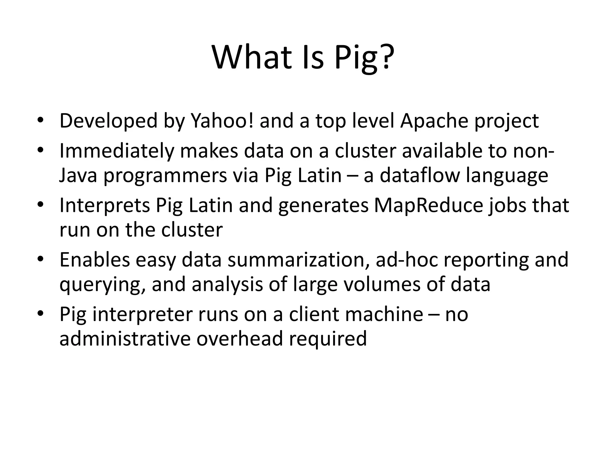
20. ORDER. . .BY
• Use the ORDER…BY operator to sort a relation
based on one or more fields
• Basic syntax:
alias = ORDER alias BY field_alias [ASC|DESC];
• Example:
DUMP alias1;
(1,2,3) (4,2,1) (8,3,4) (4,3,3) (7,2,5) (8,4,3)
alias2 = ORDER alias1 BY col3 DESC;
DUMP alias2;
(7,2,5) (8,3,4) (1,2,3) (4,3,3) (8,4,3) (4,2,1)

21. DISTINCT. . .
• Use the DISTINCT operator to remove
duplicate tuples in a relation.
• Basic syntax:
alias2 = DISTINCT alias1;
• Example:
DUMP alias1;
(8,3,4) (1,2,3) (4,3,3) (4,3,3) (1,2,3)
alias2= DISTINCT alias1;
DUMP alias2;
(8,3,4) (1,2,3) (4,3,3)

22. Relational Operators
• FLATTEN
– Used to un-nest tuples as well as bags
• INNER JOIN
– Used to perform an inner join of two or more relations based on
common field values
• OUTER JOIN
– Used to perform left, right or full outer joins
• SPLIT
– Used to partition the contents of a relation into two or more
relations
• SAMPLE
– Used to select a random data sample with the stated sample
size

23. INNER JOIN. . .
• Use the JOIN operator to perform an inner, equi-
join join of two or more relations based on
common field values
• The JOIN operator always performs an inner join
• Inner joins ignore null keys
– Filter null keys before the join
• JOIN and COGROUP operators perform similar
functions
– JOIN creates a flat set of output records
– COGROUP creates a nested set of output records

24. INNER JOIN Example
DUMP Alias1;
(1,2,3)
(4,2,1)
(8,3,4)
(4,3,3)
(7,2,5)
(8,4,3)
DUMP Alias2;
(2,4)
(8,9)
(1,3)
(2,7)
(2,9)
(4,6)
(4,9)
Join Alias1 by Col1 to
Alias2 by Col1
Alias3 = JOIN Alias1 BY
Col1, Alias2 BY Col1;
Dump Alias3;
(1,2,3,1,3)
(4,2,1,4,6)
(4,3,3,4,6)
(4,2,1,4,9)
(4,3,3,4,9)
(8,3,4,8,9)
(8,4,3,8,9)

25. OUTER JOIN. . .
• Use the OUTER JOIN operator to perform left, right, or
full outer joins
– Pig Latin syntax closely adheres to the SQL standard
• The keyword OUTER is optional
– keywords LEFT, RIGHT and FULL will imply left outer, right
outer and full outer joins respectively
• Outer joins will only work provided the relations which
need to produce nulls (in the case of non-matching
keys) have schemas
• Outer joins will only work for two-way joins
– To perform a multi-way outer join perform multiple two-
way outer join statements

26. User-Defined Functions
• Natively written in Java, packaged as a jar file
– Other languages include JavaScript, Ruby, Groovy,
and Python
• Register the jar with the REGISTER statement
• Optionally, alias it with the DEFINE statement
REGISTER /src/myfunc.jar;
A = LOAD 'students';
B = FOREACH A GENERATE myfunc.MyEvalFunc($0);

27. DEFINE
• DEFINE can be used to work with UDFs and also
streaming commands
– Useful when dealing with complex input/output
formats
/* read and write comma-delimited data */
DEFINE Y 'stream.pl' INPUT(stdin USING PigStreaming(','))
OUTPUT(stdout USING PigStreaming(','));
A = STREAM X THROUGH Y;
/* Define UDFs to a more readable format */
DEFINE MAXNUM org.apache.pig.piggybank.evaluation.math.MAX;
A = LOAD ‘student_data’ AS (name:chararray, gpa1:float, gpa2:double);
B = FOREACH A GENERATE name, MAXNUM(gpa1, gpa2);
DUMP B;

28. References
• http://pig.apache.org

29. Apache Hive
Based on Slides by Adam Shook

30. What Is Hive?
• Developed by Facebook and a top-level Apache project
• A data warehousing infrastructure based on Hadoop
• Immediately makes data on a cluster available to non-
Java programmers via SQL like queries
• Built on HiveQL (HQL), a SQL-like query language
• Interprets HiveQL and generates MapReduce jobs that
run on the cluster
• Enables easy data summarization, ad-hoc reporting and
querying, and analysis of large volumes of data

31. What Hive Is Not
• Hive, like Hadoop, is designed for batch
processing of large datasets
• Not an OLTP or real-time system
• Latency and throughput are both high
compared to a traditional RDBMS
– Even when dealing with relatively small data (
<100 MB )

32. Data Hierarchy
• Hive is organised hierarchically into:
– Databases: namespaces that separate tables and
other objects
– Tables: homogeneous units of data with the same
schema
• Analogous to tables in an RDBMS
– Partitions: determine how the data is stored
• Allow efficient access to subsets of the data
– Buckets/clusters
• For sub-sampling within a partition
• Join optimization

33. HiveQL
• HiveQL / HQL provides the basic SQL-like
operations:
– Select columns using SELECT
– Filter rows using WHERE
– JOIN between tables
– Evaluate aggregates using GROUP BY
– Store query results into another table
– Download results to a local directory (i.e., export
from HDFS)
– Manage tables and queries with CREATE, DROP, and
ALTER

34. Primitive Data Types
Type Comments
TINYINT, SMALLINT, INT, BIGINT 1, 2, 4 and 8-byte integers
BOOLEAN TRUE/FALSE
FLOAT, DOUBLE Single and double precision real numbers
STRING Character string
TIMESTAMP Unix-epoch offset or datetime string
DECIMAL Arbitrary-precision decimal
BINARY Opaque; ignore these bytes

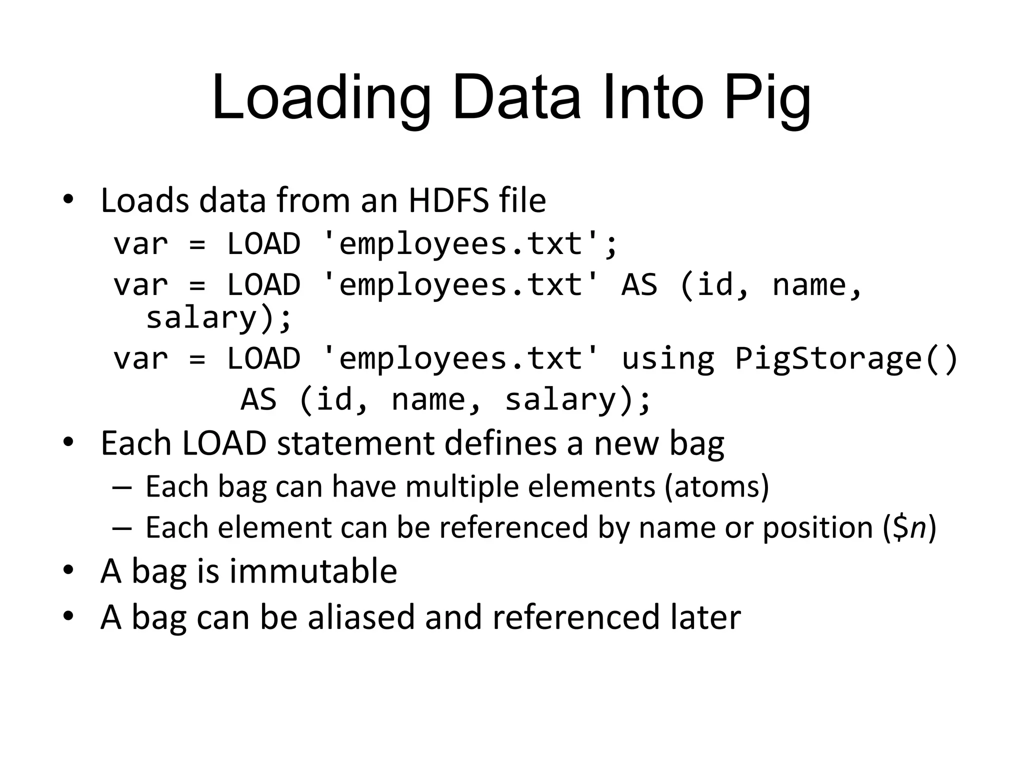
35. Complex Data Types
Type Comments
STRUCT A collection of elements
If S is of type STRUCT {a INT, b INT}:
S.a returns element a
MAP Key-value tuple
If M is a map from 'group' to GID:
M['group'] returns value of GID
ARRAY Indexed list
If A is an array of elements ['a','b','c']:
A[0] returns 'a'

36. HiveQL Limitations
• HQL only supports equi-joins, outer joins, left
semi-joins
• Because it is only a shell for Map-Reduce,
complex queries can be hard to optimise
• Missing large parts of full SQL specification:
– HAVING clause in SELECT
– Correlated sub-queries
– Sub-queries outside FROM clauses
– Updatable or materialized views
– Stored procedures

37. Hive Metastore
• Stores Hive metadata
• Default metastore database uses Apache Derby
• Various configurations:
– Embedded (in-process metastore, in-process
database)
• Mainly for unit tests
– Local (in-process metastore, out-of-process database)
• Each Hive client connects to the metastore directly
– Remote (out-of-process metastore, out-of-process
database)
• Each Hive client connects to a metastore server, which
connects to the metadata database itself

38. Hive Warehouse
• Hive tables are stored in the Hive
“warehouse”
– Default HDFS location: /user/hive/warehouse
• Tables are stored as sub-directories in the
warehouse directory
• Partitions are subdirectories of tables
• External tables are supported in Hive
• The actual data is stored in flat files

39. Hive Schemas
• Hive is schema-on-read
– Schema is only enforced when the data is read (at
query time)
– Allows greater flexibility: same data can be read
using multiple schemas
• Contrast with an RDBMS, which is schema-on-
write
– Schema is enforced when the data is loaded
– Speeds up queries at the expense of load times

40. Create Table Syntax
CREATE TABLE table_name
(col1 data_type,
col2 data_type,
col3 data_type,
col4 datatype )
ROW FORMAT DELIMITED
FIELDS TERMINATED BY ','
STORED AS format_type;

41. Simple Table
CREATE TABLE page_view
(viewTime INT,
userid BIGINT,
page_url STRING,
referrer_url STRING,
ip STRING COMMENT 'IP Address of the User' )
ROW FORMAT DELIMITED
FIELDS TERMINATED BY 't'
STORED AS TEXTFILE;

42. More Complex Table
CREATE TABLE employees (
(name STRING,
salary FLOAT,
subordinates ARRAY<STRING>,
deductions MAP<STRING, FLOAT>,
address STRUCT<street:STRING,
city:STRING,
state:STRING,
zip:INT>)
ROW FORMAT DELIMITED
FIELDS TERMINATED BY 't'
STORED AS TEXTFILE;

43. External Table
CREATE EXTERNAL TABLE page_view_stg
(viewTime INT,
userid BIGINT,
page_url STRING,
referrer_url STRING,
ip STRING COMMENT 'IP Address of the User')
ROW FORMAT DELIMITED
FIELDS TERMINATED BY 't'
STORED AS TEXTFILE
LOCATION '/user/staging/page_view';

44. More About Tables
• CREATE TABLE
– LOAD: file moved into Hive’s data warehouse directory
– DROP: both metadata and data deleted
• CREATE EXTERNAL TABLE
– LOAD: no files moved
– DROP: only metadata deleted
– Use this when sharing with other Hadoop
applications, or when you want to use multiple
schemas on the same data

45. Partitioning
• Can make some queries faster
• Divide data based on partition column
• Use PARTITION BY clause when creating table
• Use PARTITION clause when loading data
• SHOW PARTITIONS will show a table’s
partitions

46. Bucketing
• Can speed up queries that involve sampling
the data
– Sampling works without bucketing, but Hive has
to scan the entire dataset
• Use CLUSTERED BY when creating table
– For sorted buckets, add SORTED BY
• To query a sample of your data, use
TABLESAMPLE

47. Browsing Tables And Partitions
Command Comments
SHOW TABLES; Show all the tables in the database
SHOW TABLES 'page.*'; Show tables matching the
specification ( uses regex syntax )
SHOW PARTITIONS page_view; Show the partitions of the page_view
table
DESCRIBE page_view; List columns of the table
DESCRIBE EXTENDED page_view; More information on columns (useful
only for debugging )
DESCRIBE page_view
PARTITION (ds='2008-10-31');
List information about a partition

48. Loading Data
• Use LOAD DATA to load data from a file or
directory
– Will read from HDFS unless LOCAL keyword is
specified
– Will append data unless OVERWRITE specified
– PARTITION required if destination table is partitioned
LOAD DATA LOCAL INPATH '/tmp/pv_2008-06-8_us.txt'
OVERWRITE INTO TABLE page_view
PARTITION (date='2008-06-08', country='US')

49. Inserting Data
• Use INSERT to load data from a Hive query
– Will append data unless OVERWRITE specified
– PARTITION required if destination table is
partitioned
FROM page_view_stg pvs
INSERT OVERWRITE TABLE page_view
PARTITION (dt='2008-06-08', country='US')
SELECT pvs.viewTime, pvs.userid,
pvs.page_url, pvs.referrer_url
WHERE pvs.country = 'US';

50. Loading And Inserting Data: Summary
Use this For this purpose
LOAD Load data from a file or directory
INSERT Load data from a query
• One partition at a time
• Use multiple INSERTs to insert into
multiple partitions in the one query
CREATE TABLE AS (CTAS) Insert data while creating a table
Add/modify external file Load new data into external table

51. Sample Select Clauses
• Select from a single table
SELECT *
FROM sales
WHERE amount > 10 AND
region = "US";
• Select from a partitioned table
SELECT page_views.*
FROM page_views
WHERE page_views.date >= '2008-03-01' AND
page_views.date <= '2008-03-31'

52. Relational Operators
• ALL and DISTINCT
– Specify whether duplicate rows should be returned
– ALL is the default (all matching rows are returned)
– DISTINCT removes duplicate rows from the result set
• WHERE
– Filters by expression
– Does not support IN, EXISTS or sub-queries in the
WHERE clause
• LIMIT
– Indicates the number of rows to be returned

53. Relational Operators
• GROUP BY
– Group data by column values
– Select statement can only include columns
included in the
GROUP BY clause
• ORDER BY / SORT BY
– ORDER BY performs total ordering
• Slow, poor performance
– SORT BY performs partial ordering
• Sorts output from each reducer

54. Advanced Hive Operations
• JOIN
– If only one column in each table is used in the join, then
only one MapReduce job will run
• This results in 1 MapReduce job:
SELECT * FROM a JOIN b ON a.key = b.key JOIN c ON b.key = c.key
• This results in 2 MapReduce jobs:
SELECT * FROM a JOIN b ON a.key = b.key JOIN c ON b.key2 = c.key
– If multiple tables are joined, put the biggest table last and
the reducer will stream the last table, buffer the others
– Use left semi-joins to take the place of IN/EXISTS
SELECT a.key, a.val FROM a LEFT SEMI JOIN b on a.key = b.key;

55. Advanced Hive Operations
• JOIN
– Do not specify join conditions in the WHERE clause
• Hive does not know how to optimise such queries
• Will compute a full Cartesian product before filtering it
• Join Example
SELECT
a.ymd, a.price_close, b.price_close
FROM stocks a
JOIN stocks b ON a.ymd = b.ymd
WHERE a.symbol = 'AAPL' AND
b.symbol = 'IBM' AND
a.ymd > '2010-01-01';

56. Hive Stinger
• MPP-style execution of Hive queries
• Available since Hive 0.13
• No MapReduce
• We will talk about this more when we get to
SQL on Hadoop

57. References
• http://hive.apache.org