
Recommended
Recommended
More Related Content
Similar to Physics teacher support material 1Investigation 6Pag.docx
Similar to Physics teacher support material 1Investigation 6Pag.docx (8)
More from mattjtoni51554
More from mattjtoni51554 (20)
Recently uploaded
Recently uploaded (20)
Physics teacher support material 1Investigation 6Pag.docx
- 1. Physics teacher support material 1 Investigation 6 Page 1 Physical and mathematical models of the greenhouse effect My Research Questions If the Earth had no atmosphere, its average surface temperature would be about –18°C. However, the heat trapping effect of the atmosphere, called the greenhouse effect, means that a dynamic equilibrium occurs around 14°C, and thus we can live a sustainable life on earth.(1) The visible and short‐infrared radiation from the sun passes easily through the atmosphere and warms the earth’s surface. However, being cooler than the sun, the earth’s surface radiates back at a longer infrared wavelength. Moleculesof water vapor and carbon dioxide in the atmosphere absorb someof this radiation. These then emit infrared radiation in all directions, including back towards the earth. The atmosphere and the earth’s surface both warm up until a higher equilibrium temperature
- 2. is reached. As more of the atmosphere absorbs and re‐radiates heat, the overall temperature of the earthincreases. This effect is called global‐warming. By burning fossil fuels, industrial societies like Western Europe and the Americas are putting carbon dioxide into the atmosphere at a faster rate than plants can absorb it. This is adding to the greenhouse effect, hence an enhanced greenhouse effect occurs, and this may be causing global warming. There is strong evidence that the average temperature of the earthis increasing. Although the effects of global warming cannot be predicted with any certainty, this phenomenon is worthy of further study. Moreover,when we covered the physics topic8.2 “Thermal energy transfer” we learned the basics of the greenhouse effect, the enhanced greenhouse effect, the energy balance in the earthsurface‐atmosphere system, climate change and (my biggest concern) global warming. My passion for saving the environment and education people about the dangers of global warming have been developed in my physics IA project. I had two approaches in mind, and my teacher encouraged me to follow both physical and mathematical models of the greenhouse effect. The purpose of my physics exploration is two‐fold. First, I want to demonstrate global warming by a physical model. This will consist of
- 3. two largesoda bottles, one with flat soda and another with fizzysoda. The fizzysoda will produce an atmosphere with CO2 while the flat soda will not. Both bottles are then set in direct sunlight for an hour and a record of the temperatures of each are recorded. The CO2 atmosphere bottle ends up with a higher equilibrium temperature, thus demonstrating the greenhouse effect, the enhanced greenhouse effect and so demonstrating global warming. The second part of this exploration is to produce a simple one‐dimensional mathematical model of the atmosphere. This is done in Excel. The various parameters affecting the balanced or equilibrium temperature are explored. Physics teacher support material 2 Investigation 6 Page 2 A PHYSICAL MODEL OF THE GREENHOUSE EFFECT My physical model of the greenhouse effect consisted of two identical plastic bottles set in the sun but one bottle had flat soda in it and the otherhad fresh, fizzysoda producing an atmosphere of CO2 in it.(3)I then measured the
- 4. temperature over time and observed the effect of the different atmospheres on the absorption of heat from the sun. I took two identical 2‐liter clear plastic soda drink bottles and fitted them each with thermometer probes connected to a Vernier’s LabPro interface data logger unit and then into my computer using Vernier’s LoggerPro graphing software.(4) Next I took two identical 12 once bottles of soda at roomtemperature and opened one and poured it into a largemixing bowl. I agitated the soda until all the fizz was gone. This was the flat or non‐CO2 soda. Using a funnel I filled one of the 2‐litre bottles with the flat soda and then opened a freshbottle of soda and poured it into the second 2‐litre bottle. Both bottles were situated in the direct sunlight. I started data logging and sealed the bottle caps with the thermometer leadspassing through a small hole in the lid. I recorded the temperature every two seconds for about an hour. As expected, I found that the CO2 bottle retained slightly more of the radiant energy from the sun and hence had a higher temperature. Graph 1 is a closeup of the first minute of data, and as you can see therewas no temperature change
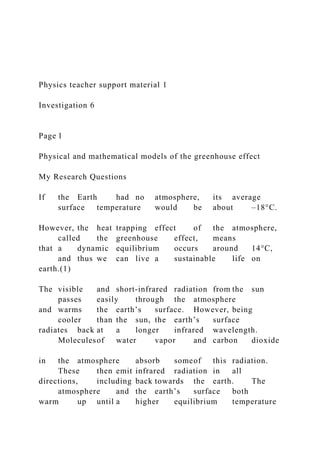
- 5. for about the first ten seconds. It took this long to prepare the bottles. Soonafter this the temperatures of both bottles started rising, and by 20 seconds the CO2 bottle was getting warmer the non‐C02 bottle. Photograph of the setup. Above: Photograph of experimental setup, outside in the sun. Right: Graph 1, A Close Up of Temperature and time for the first 50 seconds. Graph 2 (below) is temperature against time for about an hour. The CO2 bottle is always slightly warmer than the flat soda bottle. Eventually they both reach equilibrium, but not at the same temperature. The CO2 bottle remains about one‐half a degree higher compared to the non‐C02 bottle. The small blip around 2766 seconds was due to a cloud passing overhead.
- 6. Physics teacher support material 3 Investigation 6 Page 3 Graph 2: Temperature and Time for Entire Run Graph 3: Equilibrium Temperatures In Graph 3, the upper line is soda with CO2 and the lower black line is flat soda. Soonafter 3210 seconds both bottles reached equilibrium temperatures. The typical temperature difference was around 0.5 C. The slight fluctuation may be due to thermal noise, and does not really make any difference in my results. This experiment was performedseveral times and the temperature variation ranged from 1 C° to about 0.5° difference. Graph 4 is an example where the difference was the greatest, one‐degree, and it was performedon a different day.
- 7. The upper line in Graph 4 is soda with CO2 and the lower red line is flat soda. In this run, I did not start recording temperature until the bottles were filled and set out in the sun. It was difficult to read the computer screen in bright sunlight, but the resulting graph clearly shows that the atmosphere in the C02 bottle retained more heat compared to the flat soda atmosphere. Graph 4: Temperature and Time, Another Data Set In conclusion, both bottles mimic the greenhouse effect, and the CO2 bottle mimics the enhanced greenhouse effect—hence global warming— with a higher temperature, even at equilibrium, than the non‐CO2 bottle. My purpose was qualitative only.My physical model was for pedagogical uses, to illustrate with a hands‐on approach the greenhouse effect. It was not to model planetary atmosphere but to provide a simple hand‐on demonstration of the effects of greenhouse gases. The differences between the demonstration and planetary atmosphere are very complex but not relevant to this inquiry; errors and uncertainties need not be measured. However, sources of error include a slight agitating when filling the bottle to the flat bottle of soda that causes someCO2; not starting at the same temperature (which is difficult); placing the two bottle in identical sunlight locations, with no shadow of one on
- 8. the other; having the bottle on the same surface; and theremay be somegas escaping from the lid and temperature probe connection. Further extensions might include recording data for several days (includingthe nighttime); building a larger container and adding living plants. Physics teacher support material 4 Investigation 6 Page 4 Although the hands‐on model conclusions are exciting, a mathematical model is needed. We now turn to a mathematical model of the greenhouse effect. A MATHEMATICAL MODEL OF THE GREENHOUSE EFFECT Next I produced a Microsoft(5) Excel spreadsheet program using the physics equations of solar radiation and the relevant greenhouse effect equations.The first spreadsheet investigation (spreadsheet A) starts with the earth’s temperature at 0°C and accepts the standard values of solar radiation, emissivityand albedo. I then progress in one‐year steps to determine how long it takesfor the earth’s temperature to reach equilibrium.
- 9. The second spreadsheet investigation (spreadsheet B) continues this exploration by selecting a range of different starting temperature from very cold to very hot and then determines the time it takesto reach equilibrium. The third spreadsheet investigation (spreadsheet C) varies of value of the earth’s emissivityand then determines the time to reach equilibrium. The fourth spreadsheet investigation (spreadsheet D) increases the C02 content and hence demonstrates the growing nature of the enhanced greenhouse effect and thus also demonstrates global warming. Unfortunately, the technical details here proved beyond the scope of my inquiry, and my results were unrealistic. Technical Terms and Equations Instead of footnoting each equation or numerical value I simply mention here that I used Wikipediaas a source of constant values and my IB physics textbook for the relevant equations.(6) The equations involving temperature use the absolute or Kelvin scalebut I graph the results using the Celsius scale. The conversion is straightforward.
- 10. 3.15 Stefan‐Boltzmann Constant (sigma, is a constant of proportionality relating the total energy radiated per unit surface area of a black body in unit time;the S‐F law states a proportionality to the fourth power of the thermodynamictemperature. The constant is: The solar constant ( Ksolar ) for the earthis the solar power (electromagnetic radiation) per unit area. It has an approximate but accepted value. However, the total power received by the earthis proportional to the crosssectional Physics teacher support material 5 Investigation 6 Page 5 area On average this power is distributed over the surface of the earththat is
- 11. 2 . To get the average power per square meter we therefore need to divide the solar constant by 4. This is explained on the Wikipediaweb site for the solar constant. Hence I do this in the relevant equations,such as: Ksolar 4 4 At the surface of the earth, the albedo is the ratio between the incoming radiation intensity and the amount reflected expressed as a coefficient or percentage. The value varies with surface material but an overall average for the earthis given. The absorbed solar radiation per square meter Iin is therefore:
- 12. Ksolar 4 Ksolar 4 4 The emissivity of a material is the relative ability of its surface to emit energy by radiation. It is the ratio of energy radiated by a given material to the energy radiated by an ideal or black body at the same temperature. A true black body would have but for all otherreal bodies The emitted radiation of the earththus depends on the average or emissivity, and can be taken as: The Stefan‐Boltzmann Law for a given surface area of one square meter can thus express the emitted radiation Iout of the earthon average. Temperature T is on the Kelvin scale. 4
- 13. For the earthat a temperature of 0°C this gives an value of: When the radiation intensity coming into the earth just equals the intensity going out, we have a state of equilibrium. For the earththis equilibrium turnsout to be about 14°C. We can solve for this as follows. 4 4
- 14. Physics teacher support material 6 Investigation 6 Page 6 When the inputand output radiation are not in equilibrium then it is a disturbed state, and here the net radiation absorbed ( I net ) (also in units of is simply the difference between the incoming and outgoing energy intensities: An example of the net radiation absorbed at time zero to one year is: The general equation for surface heat capacity is Q The energy is Q and the surface area is A
- 15. and the change in temperature is on the Kelvin scale, where C is the specific heat capacity. Here, however, we will understand surface heat capacity per unit area, hence the equation for the earth’s surface heat capacity will be: Surface heat capacity of the earthis the heat required to raise the temperature of a unit area of a surface by one Kelvin, in units of watts years per square meter per Kelvin. The average global heat capacity C has been estimated in terms of power for a year (recall that energy = power x time) for a unit area and a unit of temperature. Cearth surface one ye I now writean expression for the change in temperature per unit area over one year for the earth’s surface as follows:
- 16. For the first year starting at T = 0°C we find the temperature change as follows: Qone year per unit area Csurface Inet tyear Csurface In the first year, with starting temperature 0 °C, the change in temperature would be about 2.5 K, so the new temperature would be 2.5 °C. Excel Equations Here are the equations I used in the spreadsheet. Starting Temperature of 0°C on Kelvin scalein cell D2: 273.15 The year progression is generated by cell C3: =C2+1
- 17. Physics teacher support material 7 Investigation 6 Page 7 I(out) in cell E2: =(0.0000000567)*(0.612)*(D2+273.15)^4 Iout at starting temperature of 0°C is: I(net) in cell F2: =(235.8075)-E2 Inet at starting temperatures of 0°C is: The change in temperature T at year intervals is calculated as D3: =D2+(F2/16.9) At the end of the first interval this is equal to:
- 18. Inet C 42.6377 16.9 Spreadsheet A—Time to Reach Equilibrium The following is the textbook model of the earth. The solar constant is 1367 W m–2 and the albedo ratio is 0.31 with an emissivityof 0.613. The earth’s surface heat capacity is taken as 16.9 W yr m–2 K–1. The data runs from a starting temperature of 0°C for 60 years, more than enough time to find the equilibrium temperature. Here (on the right) is a sample of my data. And on for 60 years.
- 19. Physics teacher support material 8 Investigation 6 Page 8 Here is the graph of the earth’s temperature as a function of time based on the above model. Earth’s Temperature against Time The time to reach equilibrium is approximately 25 years. When looking at threesignificant figures, the temperature of 13.9°C is reached after 26 year. Looking at the equilibrium temperature to threedecimal places, however, it takes43 years to reach 13.964°C. Spreadsheet B—Different Starting Temperatures and Equilibrium Time In the next investigation I varied the initial temperature from –250°C to +250°C and then I determined the relationship between the starting temperature of the earthand the number
- 20. of years it took to reach equilibrium. The results are interesting. Time to Reach Equilibrium as a Function of Starting Temperature Range from –250°C to +250°C This graph indicates the time in years to reach equilibrium with different starting temperatures. Given the initial parameters for the earth, the natural equilibrium is around 14°Cso a starting temperature at 14°Cwould require no time to reach equilibrium. The actual equilibrium temperature has been calculated to be 13.965 °C. It is interesting to note that the curve is not symmetrical on either side of the equilibrium position. In one case the earthis warming up and the otherit is cooling down. Physics teacher support material 9 Investigation 6 Page 9
- 21. Spreadsheet C—Different Emissivity Values and Equilibrium Temperature In the next investigation I varied the emissivity ratio from low to high and then I revealed a relationship between emissivityand equilibrium temperature. Equilibrium Temperature as a Function of Emissivity Ratio In the above graph, the emissivityratio ranges from 0.10 to 0.99 revealing an equilibrium range from 177°C to –18.6°C. This is what you would expect: a decreasing equilibrium temperature as more of the intensity of incident radiation is reflected outwards. Spreadsheet D—Adding CO2 to the Model In my last investigation I made the model more realistic. My othermathematical models were simplified, of course, when compared to the real world. First, they are one‐ dimensional whereas the earth’s atmosphere is three‐dimensional; second, they took steps on one year intervals whereas in the real world the process is continuous; and third, most importantly, my model assumed greenhouse gases were constant, which they are not. A more realistic model would add a factor for the increasingC02 and othergreenhouse gases as a function of time.I should add a
- 22. factor to account for the every increasing rate of CO2. The net result would be a higher equilibrium temperature, and a more dynamic process. We are told in a Wikipediaarticle that if the CO2 level were to double then the temperature would increase by +3K. There is a mathematical factor called “radiative forcing” that increases the rate of the greenhouse gases. The equation is only an approximation to the first order, but it would be interesting to use this in my model. The equation is: C C0 where (a proportionality constant for the earth) and C is the CO2 concentration and C0 is the concentration reference. See the Carbon Dioxide Information Analysis Center
- 23. Physics teacher support material 10 Investigation 6 Page 10 (CDIAC) online at http://cdiac.ornl.gov/pns/current_ghg.html and see the Wikipediaarticle on Radiative Forcing. Here is one example of a calculation. Over 250 years ago, in 1750, the CO2 content was about 280 parts per million, and today it is 388.5 ppm. The ratio or the increase is thus: 1.3875, and so the temperature change over this period is about 1.4 K. C0
- 24. 280 Here is my graph of temperature against time with enhanced greenhouse gas.
- 25. Temperature against Time for (+) Fixed Amount of C02 and My original model had a fixedvalue for CO2, and had an equilibrium temperature of 13.96°C. See the cross(+) data points on the graph. They represent my original data. When I added a factor that increased CO2 each year, the equilibrium temperature was higher, this time at 15.34°C. See the black circle data points on the graph. This does not compare to the accepted value of temperature increase, which over the past 100 year was +0.8 °C. My model had an increase of 1.38 K, way too much as it represents a CO2 increase of about 50%.My model needs serious work. However, this last part of my mathematical model is left for future studies. Footnotes (1) Various textbooks and web sites were consulted for the general information in this study. The same or similar details can be found from many different sources. Here are the main sources of information I
- 26. consulted for this study. “Elementary Climate Physics” by F. W. Taylor (Oxford University Press, 2006), Chapters 1 and 7. “Physics for the IB Diploma” by K.A. Tsokos (5th edition, Cambridge University Press), Topic 7. “Physics for use with the IB Diploma Programme” by G. Kerr and P. Ruth, (3rd edition, IBID Press), Chapter 8. http://www.esrl.noaa.gov/gmd/outreach/lesson_plans/Modeling %20the%20Greenhouse%20Effect.pdf http://passporttoknowledge.com/scic/greenhouseeffect/educators /greenhouseeffect.pdf Physics teacher support material 11 Investigation 6
- 27. Page 11 http://www.espere.net/Unitedkingdom/water/uk_watexpgreenho use.htm http://www.wested.org//earthsystems/energy/greenhouse.html (2) The best Internet simulation for the greenhouse effect can be found at the University of Colorado at Boulder web site for Physics Education Technology, PhET. http://phet.colorado.edu/ Other simulations include: http://earthguide.ucsd.edu/earthguide/diagrams/greenhouse / and http://epa.gov/climatechange/kids/global_warming_version2.ht ml (3) My initial idea camefrom a slightly different experiment but one using a similar technique and this can be found at http://www.ucar.edu/learn/1_3_2_12t.htm. Further research revealed two excellent sources of technical help and ideas: “Greenhouse Effect Study Apparatus,” American Journal of Physics, Volume 41, #442, March 1973, and “A Simple Experiment to Demonstrate the Effects of
- 28. Greenhouse Gases” by C. F. Keating in The Physics Teacher Volume 45, September 2007, pages 376 to 378. (4) Vernier hardware and software information can be found at http://www.vernier.com/. Note that I used the Surface Temperature Sensor and not the Temperature Probe because the surface sensor is better suited for low‐density measurements, like air. (5) http://office.microsoft.com/en‐us/excel/ (6) For numerical values with as many as possible decimal places, I used Wikipediaas a source (http://en.wikipedia.org/) and my textbook “Physics for the IB Diploma” by K.A. Tsokos (Cambridge Press) for the relevant equations. Physics teacher support material 1 Investigation 6 Page 1
- 29. Physical and mathematical models of the greenhouse effect My Research Questions If the Earth had no atmosphere, its average surface temperature would be about –18°C. However, the heat trapping effect of the atmosphere, called the greenhouse effect, means that a dynamic equilibrium occurs around 14°C, and thus we can live a sustainable life on earth.(1) The visible and short‐infrared radiation from the sun passes easily through the atmosphere and warms the earth’s surface. However, being cooler than the sun, the earth’s surface radiates back at a longer infrared wavelength. Moleculesof water vapor and carbon dioxide in the atmosphere absorb someof this radiation. These then emit infrared radiation in all directions, including back towards the earth. The atmosphere and the earth’s surface both warm up until a higher equilibrium temperature is reached. As more of the atmosphere absorbs and re‐radiates heat, the overall temperature of the earthincreases. This effect is called global‐warming. By burning fossil fuels, industrial societies like Western Europe and the Americas are putting carbon dioxide into the atmosphere at a faster rate than plants can absorb it. This is adding to the greenhouse effect, hence an
- 30. enhanced greenhouse effect occurs, and this may be causing global warming. There is strong evidence that the average temperature of the earthis increasing. Although the effects of global warming cannot be predicted with any certainty, this phenomenon is worthy of further study. Moreover,when we covered the physics topic8.2 “Thermal energy transfer” we learned the basics of the greenhouse effect, the enhanced greenhouse effect, the energy balance in the earthsurface‐atmosphere system, climate change and (my biggest concern) global warming. My passion for saving the environment and education people about the dangers of global warming have been developed in my physics IA project. I had two approaches in mind, and my teacher encouraged me to follow both physical and mathematical models of the greenhouse effect. The purpose of my physics exploration is two‐fold. First, I want to demonstrate global warming by a physical model. This will consist of two largesoda bottles, one with flat soda and another with fizzysoda. The fizzysoda will produce an atmosphere with CO2 while the flat soda will not. Both bottles are then set in direct sunlight for an hour and a record of the temperatures of each are recorded. The CO2 atmosphere bottle ends up with a higher equilibrium temperature, thus demonstrating the greenhouse effect, the enhanced greenhouse effect and so demonstrating global warming.
- 31. The second part of this exploration is to produce a simple one‐dimensional mathematical model of the atmosphere. This is done in Excel. The various parameters affecting the balanced or equilibrium temperature are explored. Physics teacher support material 2 Investigation 6 Page 2 A PHYSICAL MODEL OF THE GREENHOUSE EFFECT My physical model of the greenhouse effect consisted of two identical plastic bottles set in the sun but one bottle had flat soda in it and the otherhad fresh, fizzysoda producing an atmosphere of CO2 in it.(3)I then measured the temperature over time and observed the effect of the different atmospheres on the absorption of heat from the sun. I took two identical 2‐liter clear plastic soda drink bottles and fitted them each with thermometer probes connected to a Vernier’s LabPro interface data logger unit and then into my computer using Vernier’s LoggerPro graphing software.(4)
- 32. Next I took two identical 12 once bottles of soda at roomtemperature and opened one and poured it into a largemixing bowl. I agitated the soda until all the fizz was gone. This was the flat or non‐CO2 soda. Using a funnel I filled one of the 2‐litre bottles with the flat soda and then opened a freshbottle of soda and poured it into the second 2‐litre bottle. Both bottles were situated in the direct sunlight. I started data logging and sealed the bottle caps with the thermometer leadspassing through a small hole in the lid. I recorded the temperature every two seconds for about an hour. As expected, I found that the CO2 bottle retained slightly more of the radiant energy from the sun and hence had a higher temperature. Graph 1 is a closeup of the first minute of data, and as you can see therewas no temperature change for about the first ten seconds. It took this long to prepare the bottles. Soonafter this the temperatures of both bottles started rising, and by 20 seconds the CO2 bottle was getting warmer the non‐C02 bottle. Photograph of the setup.
- 33. Above: Photograph of experimental setup, outside in the sun. Right: Graph 1, A Close Up of Temperature and time for the first 50 seconds. Graph 2 (below) is temperature against time for about an hour. The CO2 bottle is always slightly warmer than the flat soda bottle. Eventually they both reach equilibrium, but not at the same temperature. The CO2 bottle remains about one‐half a degree higher compared to the non‐C02 bottle. The small blip around 2766 seconds was due to a cloud passing overhead. Physics teacher support material 3 Investigation 6 Page 3
- 34. Graph 2: Temperature and Time for Entire Run Graph 3: Equilibrium Temperatures In Graph 3, the upper line is soda with CO2 and the lower black line is flat soda. Soonafter 3210 seconds both bottles reached equilibrium temperatures. The typical temperature difference was around 0.5 C. The slight fluctuation may be due to thermal noise, and does not really make any difference in my results. This experiment was performedseveral times and the temperature variation ranged from 1 C° to about 0.5° difference. Graph 4 is an example where the difference was the greatest, one‐degree, and it was performedon a different day. The upper line in Graph 4 is soda with CO2 and the lower red line is flat soda. In this run, I did not start recording temperature until the bottles were filled and set out in the sun. It was difficult to read the computer screen in bright sunlight, but the resulting graph clearly shows that the atmosphere in the C02 bottle retained more heat compared to the flat soda atmosphere.
- 35. Graph 4: Temperature and Time, Another Data Set In conclusion, both bottles mimic the greenhouse effect, and the CO2 bottle mimics the enhanced greenhouse effect—hence global warming— with a higher temperature, even at equilibrium, than the non‐CO2 bottle. My purpose was qualitative only.My physical model was for pedagogical uses, to illustrate with a hands‐on approach the greenhouse effect. It was not to model planetary atmosphere but to provide a simple hand‐on demonstration of the effects of greenhouse gases. The differences between the demonstration and planetary atmosphere are very complex but not relevant to this inquiry; errors and uncertainties need not be measured. However, sources of error include a slight agitating when filling the bottle to the flat bottle of soda that causes someCO2; not starting at the same temperature (which is difficult); placing the two bottle in identical sunlight locations, with no shadow of one on the other; having the bottle on the same surface; and theremay be somegas escaping from the lid and temperature probe connection. Further extensions might include recording data for several days (includingthe nighttime); building a larger container and adding living plants. Physics teacher support material 4
- 36. Investigation 6 Page 4 Although the hands‐on model conclusions are exciting, a mathematical model is needed. We now turn to a mathematical model of the greenhouse effect. A MATHEMATICAL MODEL OF THE GREENHOUSE EFFECT Next I produced a Microsoft(5) Excel spreadsheet program using the physics equations of solar radiation and the relevant greenhouse effect equations.The first spreadsheet investigation (spreadsheet A) starts with the earth’s temperature at 0°C and accepts the standard values of solar radiation, emissivityand albedo. I then progress in one‐year steps to determine how long it takesfor the earth’s temperature to reach equilibrium. The second spreadsheet investigation (spreadsheet B) continues this exploration by selecting a range of different starting temperature from very cold to very hot and then determines the time it takesto reach equilibrium. The third spreadsheet investigation (spreadsheet C) varies of value of the earth’s emissivityand then determines the time to reach
- 37. equilibrium. The fourth spreadsheet investigation (spreadsheet D) increases the C02 content and hence demonstrates the growing nature of the enhanced greenhouse effect and thus also demonstrates global warming. Unfortunately, the technical details here proved beyond the scope of my inquiry, and my results were unrealistic. Technical Terms and Equations Instead of footnoting each equation or numerical value I simply mention here that I used Wikipediaas a source of constant values and my IB physics textbook for the relevant equations.(6) The equations involving temperature use the absolute or Kelvin scalebut I graph the results using the Celsius scale. The conversion is straightforward. Stefan‐Boltzmann Constant (sigma, is a constant of proportionality relating the total energy radiated per unit surface area of a black body in unit time;the S‐F law states a proportionality to the fourth power of the thermodynamictemperature. The constant is:
- 38. The solar constant ( Ksolar ) for the earthis the solar power (electromagnetic radiation) per unit area. It has an approximate but accepted value. However, the total power received by the earthis proportional to the crosssectional Physics teacher support material 5 Investigation 6 Page 5 area On average this power is distributed over the surface of the earththat is 2 . To get the average power per square meter we therefore need to divide the solar constant by 4. This is explained on the Wikipediaweb site for the solar constant. Hence I do this in the relevant equations,such as:
- 39. Ksolar 4 4 At the surface of the earth, the albedo is the ratio between the incoming radiation intensity and the amount reflected expressed as a coefficient or percentage. The value varies with surface material but an overall average for the earthis given. The absorbed solar radiation per square meter Iin is therefore: Ksolar 4 Ksolar 4 4
- 40. The emissivity of a material is the relative ability of its surface to emit energy by radiation. It is the ratio of energy radiated by a given material to the energy radiated by an ideal or black body at the same temperature. A true black body would have but for all otherreal bodies The emitted radiation of the earththus depends on the average or emissivity, and can be taken as: The Stefan‐Boltzmann Law for a given surface area of one square meter can thus express the emitted radiation Iout of the earthon average. Temperature T is on the Kelvin scale. 4 For the earthat a temperature of 0°C this gives an value of: When the radiation intensity coming into the earth just equals the intensity going out, we have a state of equilibrium.
- 41. For the earththis equilibrium turnsout to be about 14°C. We can solve for this as follows. 4 4 Physics teacher support material 6 Investigation 6 Page 6
- 42. When the inputand output radiation are not in equilibrium then it is a disturbed state, and here the net radiation absorbed ( I net ) (also in units of is simply the difference between the incoming and outgoing energy intensities: An example of the net radiation absorbed at time zero to one year is: The general equation for surface heat capacity is Q The energy is Q and the surface area is A and the change in temperature is on the Kelvin scale, where C is the specific heat capacity. Here, however, we will understand surface heat capacity per unit area, hence the equation for the earth’s surface heat capacity will be:
- 43. Surface heat capacity of the earthis the heat required to raise the temperature of a unit area of a surface by one Kelvin, in units of watts years per square meter per Kelvin. The average global heat capacity C has been estimated in terms of power for a year (recall that energy = power x time) for a unit area and a unit of temperature. I now writean expression for the change in temperature per unit area over one year for the earth’s surface as follows: For the first year starting at T = 0°C we find the temperature change as follows: Qone year per unit area Csurface Inet tyear
- 44. Csurface In the first year, with starting temperature 0 °C, the change in temperature would be about 2.5 K, so the new temperature would be 2.5 °C. Excel Equations Here are the equations I used in the spreadsheet. Starting Temperature of 0°C on Kelvin scalein cell D2: 273.15 The year progression is generated by cell C3: =C2+1 Physics teacher support material 7 Investigation 6 Page 7
- 45. I(out) in cell E2: =(0.0000000567)*(0.612)*(D2+273.15)^4 Iout at starting temperature of 0°C is: I(net) in cell F2: =(235.8075)-E2 Inet at starting temperatures of 0°C is: The change in temperature T at year intervals is calculated as D3: =D2+(F2/16.9) At the end of the first interval this is equal to: Inet C
- 46. 42.6377 16.9 Spreadsheet A—Time to Reach Equilibrium The following is the textbook model of the earth. The solar constant is 1367 W m–2 and the albedo ratio is 0.31 with an emissivityof 0.613. The earth’s surface heat capacity is taken as 16.9 W yr m–2 K–1. The data runs from a starting temperature of 0°C for 60 years, more than enough time to find the equilibrium temperature. Here (on the right) is a sample of my data. And on for 60 years. Physics teacher support material 8 Investigation 6 Page 8
- 47. Here is the graph of the earth’s temperature as a function of time based on the above model. Earth’s Temperature against Time The time to reach equilibrium is approximately 25 years. When looking at threesignificant figures, the temperature of 13.9°C is reached after 26 year. Looking at the equilibrium temperature to threedecimal places, however, it takes43 years to reach 13.964°C. Spreadsheet B—Different Starting Temperatures and Equilibrium Time In the next investigation I varied the initial temperature from –250°C to +250°C and then I determined the relationship between the starting temperature of the earthand the number of years it took to reach equilibrium. The results are interesting. Time to Reach Equilibrium as a Function of Starting Temperature Range from –250°C to +250°C This graph indicates the time in years to reach
- 48. equilibrium with different starting temperatures. Given the initial parameters for the earth, the natural equilibrium is around 14°Cso a starting temperature at 14°Cwould require no time to reach equilibrium. The actual equilibrium temperature has been calculated to be 13.965 °C. It is interesting to note that the curve is not symmetrical on either side of the equilibrium position. In one case the earthis warming up and the otherit is cooling down. Physics teacher support material 9 Investigation 6 Page 9 Spreadsheet C—Different Emissivity Values and Equilibrium Temperature In the next investigation I varied the emissivity ratio from low to high and then I revealed a relationship between emissivityand equilibrium temperature. Equilibrium Temperature
- 49. as a Function of Emissivity Ratio In the above graph, the emissivityratio ranges from 0.10 to 0.99 revealing an equilibrium range from 177°C to –18.6°C. This is what you would expect: a decreasing equilibrium temperature as more of the intensity of incident radiation is reflected outwards. Spreadsheet D—Adding CO2 to the Model In my last investigation I made the model more realistic. My othermathematical models were simplified, of course, when compared to the real world. First, they are one‐ dimensional whereas the earth’s atmosphere is three‐dimensional; second, they took steps on one year intervals whereas in the real world the process is continuous; and third, most importantly, my model assumed greenhouse gases were constant, which they are not. A more realistic model would add a factor for the increasingC02 and othergreenhouse gases as a function of time.I should add a factor to account for the every increasing rate of CO2. The net result would be a higher equilibrium temperature, and a more dynamic process. We are told in a Wikipediaarticle that if the CO2 level were to double then the temperature would increase by +3K. There is a mathematical factor called “radiative forcing” that increases the rate of the greenhouse gases. The equation is only an
- 50. approximation to the first order, but it would be interesting to use this in my model. The equation is: C C0 where (a proportionality constant for the earth) and C is the CO2 concentration and C0 is the concentration reference. See the Carbon Dioxide Information Analysis Center Physics teacher support material 10 Investigation 6 Page 10 (CDIAC) online at
- 51. http://cdiac.ornl.gov/pns/current_ghg.html and see the Wikipediaarticle on Radiative Forcing. Here is one example of a calculation. Over 250 years ago, in 1750, the CO2 content was about 280 parts per million, and today it is 388.5 ppm. The ratio or the increase is thus: 1.3875, and so the temperature change over this period is about 1.4 K. C0
- 52. 280 Here is my graph of temperature against time with enhanced greenhouse gas. Temperature against Time for (+) Fixed Amount of C02 and My original model had a fixedvalue for CO2, and had an equilibrium temperature of 13.96°C. See the cross(+) data points on the graph. They
- 53. represent my original data. When I added a factor that increased CO2 each year, the equilibrium temperature was higher, this time at 15.34°C. See the black circle data points on the graph. This does not compare to the accepted value of temperature increase, which over the past 100 year was +0.8 °C. My model had an increase of 1.38 K, way too much as it represents a CO2 increase of about 50%.My model needs serious work. However, this last part of my mathematical model is left for future studies. Footnotes (1) Various textbooks and web sites were consulted for the general information in this study. The same or similar details can be found from many different sources. Here are the main sources of information I consulted for this study. “Elementary Climate Physics” by F. W. Taylor (Oxford University Press, 2006), Chapters 1 and 7. “Physics for the IB Diploma” by K.A. Tsokos (5th edition, Cambridge University Press), Topic 7.
- 54. “Physics for use with the IB Diploma Programme” by G. Kerr and P. Ruth, (3rd edition, IBID Press), Chapter 8. http://www.esrl.noaa.gov/gmd/outreach/lesson_plans/Modeling %20the%20Greenhouse%20Effect.pdf http://passporttoknowledge.com/scic/greenhouseeffect/educators /greenhouseeffect.pdf Physics teacher support material 11 Investigation 6 Page 11 http://www.espere.net/Unitedkingdom/water/uk_watexpgreenho use.htm http://www.wested.org//earthsystems/energy/greenhouse.html (2) The best Internet simulation for the greenhouse
- 55. effect can be found at the University of Colorado at Boulder web site for Physics Education Technology, PhET. http://phet.colorado.edu/ Other simulations include: http://earthguide.ucsd.edu/earthguide/diagrams/greenhouse / and http://epa.gov/climatechange/kids/global_warming_version2.ht ml (3) My initial idea camefrom a slightly different experiment but one using a similar technique and this can be found at http://www.ucar.edu/learn/1_3_2_12t.htm. Further research revealed two excellent sources of technical help and ideas: “Greenhouse Effect Study Apparatus,” American Journal of Physics, Volume 41, #442, March 1973, and “A Simple Experiment to Demonstrate the Effects of Greenhouse Gases” by C. F. Keating in The Physics Teacher Volume 45, September 2007, pages 376 to 378. (4) Vernier hardware and software information can be found at http://www.vernier.com/. Note that I used the Surface Temperature Sensor and not the
- 56. Temperature Probe because the surface sensor is better suited for low‐density measurements, like air. (5) http://office.microsoft.com/en‐us/excel/ (6) For numerical values with as many as possible decimal places, I used Wikipediaas a source (http://en.wikipedia.org/) and my textbook “Physics for the IB Diploma” by K.A. Tsokos (Cambridge Press) for the relevant equations.