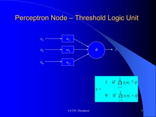
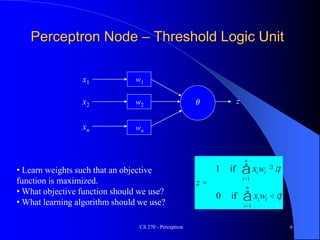
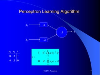
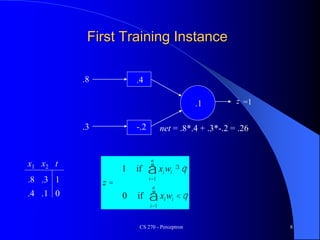
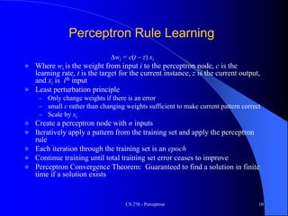
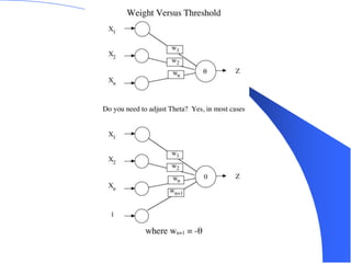
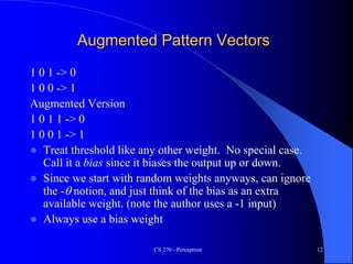
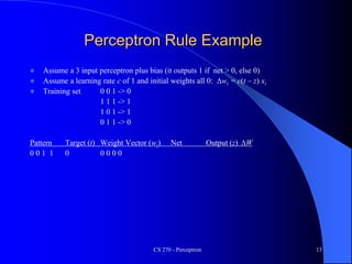
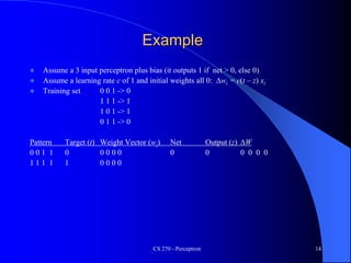
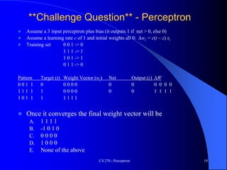
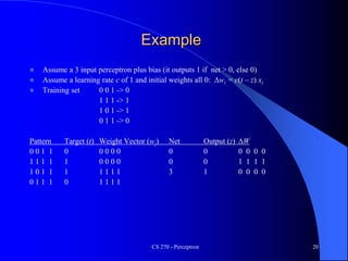
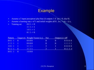
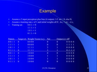
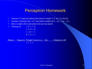
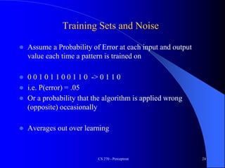
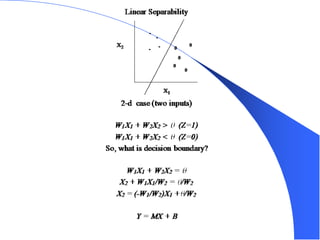
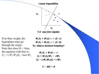
CS 270 - Perceptron 1
CS 270 - Perceptron 2
Basic Neuron
CS 270 - Perceptron 3
Expanded Neuron
CS 270 - Perceptron 4
Perceptron Learning Algorithm
 First neural network learning model in the 1960’s
– Frank Rosenblatt
 Simple and limited (single layer model)
 Basic concepts are similar for multi-layer models so this is
a good learning tool
 Still used in some current applications (large business
problems, where intelligibility is needed, etc.)
CS 270 - Perceptron 5
Perceptron Node – Threshold Logic Unit
x1
xn
x2
w1
w2
wn
z
q
q
q
<
=
³
å
å
=
=
i
n
i
i
i
n
i
i
w
x
z
w
x
1
1
if
0
if
1
𝜃
CS 270 - Perceptron 6
Perceptron Node – Threshold Logic Unit
x1
xn
x2
w1
w2
wn
z
q
q
<
=
³
å
å
=
=
i
n
i
i
i
n
i
i
w
x
z
w
x
1
1
if
0
if
1
• Learn weights such that an objective
function is maximized.
• What objective function should we use?
• What learning algorithm should we use?
𝜃
CS 270 - Perceptron 7
Perceptron Learning Algorithm
x1
x2
z
q
q
<
=
³
å
å
=
=
i
n
i
i
i
n
i
i
w
x
z
w
x
1
1
if
0
if
1
.4
-.2
.1
x1 x2 t
0
1
.1
.3
.4
.8
CS 270 - Perceptron 8
First Training Instance
.8
.3
z
q
q
<
=
³
å
å
=
=
i
n
i
i
i
n
i
i
w
x
z
w
x
1
1
if
0
if
1
.4
-.2
.1
net = .8*.4 + .3*-.2 = .26
=1
x1 x2 t
0
1
.1
.3
.4
.8
CS 270 - Perceptron 9
Second Training Instance
.4
.1
z
q
q
<
=
³
å
å
=
=
i
n
i
i
i
n
i
i
w
x
z
w
x
1
1
if
0
if
1
.4
-.2
.1
x1 x2 t
0
1
.1
.3
.4
.8
net = .4*.4 + .1*-.2 = .14
=1
Dwi = (t - z) * c * xi
CS 270 - Perceptron 10
Perceptron Rule Learning
Dwi = c(t – z) xi
 Where wi is the weight from input i to the perceptron node, c is the
learning rate, t is the target for the current instance, z is the current output,
and xi is ith input
 Least perturbation principle
– Only change weights if there is an error
– small c rather than changing weights sufficient to make current pattern correct
– Scale by xi
 Create a perceptron node with n inputs
 Iteratively apply a pattern from the training set and apply the perceptron
rule
 Each iteration through the training set is an epoch
 Continue training until total training set error ceases to improve
 Perceptron Convergence Theorem: Guaranteed to find a solution in finite
time if a solution exists
CS 270 - Perceptron 11
CS 270 - Perceptron 12
Augmented Pattern Vectors
1 0 1 -> 0
1 0 0 -> 1
Augmented Version
1 0 1 1 -> 0
1 0 0 1 -> 1
 Treat threshold like any other weight. No special case.
Call it a bias since it biases the output up or down.
 Since we start with random weights anyways, can ignore
the - notion, and just think of the bias as an extra
available weight. (note the author uses a -1 input)
 Always use a bias weight
CS 270 - Perceptron 13
Perceptron Rule Example
 Assume a 3 input perceptron plus bias (it outputs 1 if net > 0, else 0)
 Assume a learning rate c of 1 and initial weights all 0: Dwi = c(t – z) xi
 Training set 0 0 1 -> 0
1 1 1 -> 1
1 0 1 -> 1
0 1 1 -> 0
Pattern Target (t) Weight Vector (wi) Net Output (z) DW
0 0 1 1 0 0 0 0 0
CS 270 - Perceptron 14
Example
 Assume a 3 input perceptron plus bias (it outputs 1 if net > 0, else 0)
 Assume a learning rate c of 1 and initial weights all 0: Dwi = c(t – z) xi
 Training set 0 0 1 -> 0
1 1 1 -> 1
1 0 1 -> 1
0 1 1 -> 0
Pattern Target (t) Weight Vector (wi) Net Output (z) DW
0 0 1 1 0 0 0 0 0 0 0 0 0 0 0
1 1 1 1 1 0 0 0 0
CS 270 - Perceptron 15
Example
 Assume a 3 input perceptron plus bias (it outputs 1 if net > 0, else 0)
 Assume a learning rate c of 1 and initial weights all 0: Dwi = c(t – z) xi
 Training set 0 0 1 -> 0
1 1 1 -> 1
1 0 1 -> 1
0 1 1 -> 0
Pattern Target (t) Weight Vector (wi) Net Output (z) DW
0 0 1 1 0 0 0 0 0 0 0 0 0 0 0
1 1 1 1 1 0 0 0 0 0 0 1 1 1 1
1 0 1 1 1 1 1 1 1
Peer Instruction
 I pose a challenge question (often multiple choice), which
will help solidify understanding of topics we have studied
– Might not just be one correct answer
 You each get some time (1-2 minutes) to come up with
your answer and vote – use Mentimeter (anonymous)
 Then you get some time to convince your group
(neighbors) why you think you are right (2-3 minutes)
– Learn from and teach each other!
 You vote again. May change your vote if you want.
 We discuss together the different responses, show the
votes, give you opportunity to justify your thinking, and
give you further insights
CS 270 - Perceptron 16
Peer Instruction (PI) Why
 Studies show this approach improves learning
 Learn by doing, discussing, and teaching each other
– Curse of knowledge/expert blind-spot
– Compared to talking with a peer who just figured it out and who can
explain it in your own jargon
– You never really know something until you can teach it to someone
else – More improved learning!
 Learn to reason about your thinking and answers
 More enjoyable - You are involved and active in the learning
CS 270 - Perceptron 17
How Groups Interact
 Best if group members have different initial answers
 3 is the “magic” group number
– You can self-organize "on-the-fly" or sit together specifically to be a
group
– Can go 2-4 on a given day to make sure everyone is involved
 Teach and learn from each other: Discuss, reason, articulate
 If you know the answer, listen to where colleagues are coming
from first, then be a great humble teacher, you will also learn by
doing that, and you’ll be on the other side in the future
– I can’t do that as well because every small group has different
misunderstandings and you get to focus on your particular questions
 Be ready to justify to the class your vote and justifications!
CS 270 - Perceptron 18
CS 270 - Perceptron 19
**Challenge Question** - Perceptron
 Assume a 3 input perceptron plus bias (it outputs 1 if net > 0, else 0)
 Assume a learning rate c of 1 and initial weights all 0: Dwi = c(t – z) xi
 Training set 0 0 1 -> 0
1 1 1 -> 1
1 0 1 -> 1
0 1 1 -> 0
Pattern Target (t) Weight Vector (wi) Net Output (z) DW
0 0 1 1 0 0 0 0 0 0 0 0 0 0 0
1 1 1 1 1 0 0 0 0 0 0 1 1 1 1
1 0 1 1 1 1 1 1 1
 Once it converges the final weight vector will be
A. 1 1 1 1
B. -1 0 1 0
C. 0 0 0 0
D. 1 0 0 0
E. None of the above
CS 270 - Perceptron 20
Example
 Assume a 3 input perceptron plus bias (it outputs 1 if net > 0, else 0)
 Assume a learning rate c of 1 and initial weights all 0: Dwi = c(t – z) xi
 Training set 0 0 1 -> 0
1 1 1 -> 1
1 0 1 -> 1
0 1 1 -> 0
Pattern Target (t) Weight Vector (wi) Net Output (z) DW
0 0 1 1 0 0 0 0 0 0 0 0 0 0 0
1 1 1 1 1 0 0 0 0 0 0 1 1 1 1
1 0 1 1 1 1 1 1 1 3 1 0 0 0 0
0 1 1 1 0 1 1 1 1
CS 270 - Perceptron 21
Example
 Assume a 3 input perceptron plus bias (it outputs 1 if net > 0, else 0)
 Assume a learning rate c of 1 and initial weights all 0: Dwi = c(t – z) xi
 Training set 0 0 1 -> 0
1 1 1 -> 1
1 0 1 -> 1
0 1 1 -> 0
Pattern Target (t) Weight Vector (wi) Net Output (z) DW
0 0 1 1 0 0 0 0 0 0 0 0 0 0 0
1 1 1 1 1 0 0 0 0 0 0 1 1 1 1
1 0 1 1 1 1 1 1 1 3 1 0 0 0 0
0 1 1 1 0 1 1 1 1 3 1 0 -1 -1 -1
0 0 1 1 0 1 0 0 0
CS 270 - Perceptron 22
Example
 Assume a 3 input perceptron plus bias (it outputs 1 if net > 0, else 0)
 Assume a learning rate c of 1 and initial weights all 0: Dwi = c(t – z) xi
 Training set 0 0 1 -> 0
1 1 1 -> 1
1 0 1 -> 1
0 1 1 -> 0
Pattern Target (t) Weight Vector (wi) Net Output (z) DW
0 0 1 1 0 0 0 0 0 0 0 0 0 0 0
1 1 1 1 1 0 0 0 0 0 0 1 1 1 1
1 0 1 1 1 1 1 1 1 3 1 0 0 0 0
0 1 1 1 0 1 1 1 1 3 1 0 -1 -1 -1
0 0 1 1 0 1 0 0 0 0 0 0 0 0 0
1 1 1 1 1 1 0 0 0 1 1 0 0 0 0
1 0 1 1 1 1 0 0 0 1 1 0 0 0 0
0 1 1 1 0 1 0 0 0 0 0 0 0 0 0
CS 270 - Perceptron 23
Perceptron Homework
 Assume a 3 input perceptron plus bias (it outputs 1 if net > 0, else 0)
 Assume a learning rate c of 1 and initial weights all 1: Dwi = c(t – z) xi
 Show weights after each pattern for just one epoch
 Training set 1 0 1 -> 0
1 .5 0 -> 0
1 -.4 1 -> 1
0 1 .5 -> 1
Pattern Target (t) Weight Vector (wi) Net Output (z) DW
1 1 1 1
CS 270 - Perceptron 24
Training Sets and Noise
 Assume a Probability of Error at each input and output
value each time a pattern is trained on
 0 0 1 0 1 1 0 0 1 1 0 -> 0 1 1 0
 i.e. P(error) = .05
 Or a probability that the algorithm is applied wrong
(opposite) occasionally
 Averages out over learning
CS 270 - Perceptron 25
CS 270 - Perceptron 26
If no bias weight, the
hyperplane must go
through the origin.
Note that since 𝛳 = -bias,
the equation with bias is:
X2 = (-W1/W2)X1 - bias/W2
CS 270 - Perceptron 27
Linear Separability
CS 270 - Perceptron 28
Linear Separability and Generalization
When is data noise vs. a legitimate exception
CS 270 - Perceptron 29
Limited Functionality of Hyperplane
How to Handle Multi-Class Output
 This is an issue with learning models which only support binary
classification (perceptron, SVM, etc.)
 Create 1 perceptron for each output class, where the training set
considers all other classes to be negative examples (one vs the
rest)
– Run all perceptrons on novel data and set the output to the class of the
perceptron which outputs high
– If there is a tie, choose the perceptron with the highest net value
 Another approach: Create 1 perceptron for each pair of output
classes, where the training set only contains examples from the
2 classes (one vs one)
– Run all perceptrons on novel data and set the output to be the class
with the most wins (votes) from the perceptrons
– In case of a tie, use the net values to decide
– Number of models grows by the square of the output classes
CS 270 - Perceptron 30
CS 270 - Perceptron 31
UC Irvine Machine Learning Data Base
Iris Data Set
4.8,3.0,1.4,0.3, Iris-setosa
5.1,3.8,1.6,0.2, Iris-setosa
4.6,3.2,1.4,0.2, Iris-setosa
5.3,3.7,1.5,0.2, Iris-setosa
5.0,3.3,1.4,0.2, Iris-setosa
7.0,3.2,4.7,1.4, Iris-versicolor
6.4,3.2,4.5,1.5, Iris-versicolor
6.9,3.1,4.9,1.5, Iris-versicolor
5.5,2.3,4.0,1.3, Iris-versicolor
6.5,2.8,4.6,1.5, Iris-versicolor
6.0,2.2,5.0,1.5, Iris-viginica
6.9,3.2,5.7,2.3, Iris-viginica
5.6,2.8,4.9,2.0, Iris-viginica
7.7,2.8,6.7,2.0, Iris-viginica
6.3,2.7,4.9,1.8, Iris-viginica
Objective Functions: Accuracy/Error
 How do we judge the quality of a particular model (e.g.
Perceptron with a particular setting of weights)
 Consider how accurate the model is on the data set
– Classification accuracy = # Correct/Total instances
– Classification error = # Misclassified/Total instances (= 1 – acc)
 Usually minimize a Loss function (aka cost, error)
 For real valued outputs and/or targets
– Pattern error = Target – output: Errors could cancel each other
 S|tj – zj| (L1 loss), where j indexes all outputs in the pattern
 Common approach is Squared Error = S(tj – zj)2 (L2 loss)
– Total sum squared error = S pattern squared errors = S S (tij – zij)2
where i indexes all the patterns in training set
 For nominal data, pattern error is typically 1 for a mismatch and
0 for a match
– For nominal (including binary) output and targets, L!, L2, and
classification error are equivalent
CS 270 - Perceptron 32
Mean Squared Error
 Mean Squared Error (MSE) – SSE/n where n is the number of
instances in the data set
– This can be nice because it normalizes the error for data sets of
different sizes
– MSE is the average squared error per pattern
 Root Mean Squared Error (RMSE) – is the square root of the
MSE
– This puts the error value back into the same units as the features and
can thus be more intuitive
 Since we squared the error on the SSE
– RMSE is the average distance (error) of targets from the outputs in the
same scale as the features
– Note RMSE is the root of the total data set MSE, and NOT the sum of
the root of each individual pattern MSE
CS 270 - Perceptron 33
**Challenge Question** - Error
 Given the following data set, what is the L1 (S|ti – zi|), SSE (L2)
(S(ti – zi)2), MSE, and RMSE error for the entire data set?
CS 270 - Perceptron 34
x y Output Target Data Set
2 -3 1 1
0 1 0 1
.5 .6 .8 .2
L1 ?
SSE ?
MSE ?
RMSE ?
A. .4 1 1 1
B. 1.6 2.36 1 1
C. .4 .64 .21 0.453
D. 1.6 1.36 .67 .82
E. None of the above
**Challenge Question** - Error
CS 270 - Perceptron 35
x y Output Target Data Set
2 -3 1 1
0 1 0 1
.5 .6 .8 .2
L1 1.6
SSE 1.36
MSE 1.36/3 = .453
RMSE .45^.5 = .67
A. .4 1 1 1
B. 1.6 2.36 1 1
C. .4 .64 .21 0.453
D. 1.6 1.36 .67 .82
E. None of the above
 Given the following data set, what is the L1 (S|ti – zi|), SSE (L2)
(S(ti – zi)2), MSE, and RMSE error for the entire data set?
Error Values Homework
 Given the following data set, what is the L1, SSE (L2), MSE,
and RMSE error of Output1, Output2, and the entire data set?
Fill in cells that have a ?.
– Notes: For instance 1 the L1 pattern error is 1 + .6 = 1.6 and the SSE
pattern error is 1 + .16 = 1.16. The Data Set L1 and SSE errors will
just be the sum of each of the pattern errors.
CS 270 - Perceptron 36
Instance x y Output1 Target1 Output2 Target 2 Data Set
1 -1 -1 0 1 .6 1.0
2 -1 1 1 1 -.3 0
3 1 -1 1 0 1.2 .5
4 1 1 0 0 0 -.2
L1 ? ? ?
SSE ? ? ?
MSE ? ? ?
RMSE ? ? ?
CS 270 - Perceptron 37
Gradient Descent Learning: Minimize
(Maximize) the Objective Function
Total SSE:
Sum
Squared
Error
S (t – z)2
0
Error Landscape
Weight Values
CS 270 - Perceptron 38
 Goal is to decrease overall error (or other loss function)
each time a weight is changed
 Total Sum Squared error one possible loss function
E: S (t – z)2
 Seek a weight changing algorithm such that is
negative
 If a formula can be found then we have a gradient descent
learning algorithm
 Delta rule is a variant of the perceptron rule which gives a
gradient descent learning algorithm with perceptron nodes
Deriving a Gradient Descent Learning
Algorithm
ij
w
E


CS 270 - Perceptron 39
Delta rule algorithm
 Delta rule uses (target - net) before the net value goes through the
threshold in the learning rule to decide weight update
 Weights are updated even when the output would be correct
 Because this model is single layer and because of the SSE objective
function, the error surface is guaranteed to be parabolic with only one
minima
 Learning rate
– If learning rate is too large can jump around global minimum
– If too small, will get to minimum, but will take a longer time
– Can decrease learning rate over time to give higher speed and still
attain the global minimum (although exact minimum is still just for
training set and thus…)
Dwi = c(t -net)xi
Batch vs Stochastic Update
 To get the true gradient with the delta rule, we need to sum
errors over the entire training set and only update weights
at the end of each epoch
 Batch (gradient) vs stochastic (on-line, incremental)
– SGD (Stochastic Gradient Descent)
– With the stochastic delta rule algorithm, you update after every pattern,
just like with the perceptron algorithm (even though that means each
change may not be along the true gradient)
– Stochastic is more efficient and best to use in almost all cases, though not
all have figured it out yet
– We’ll talk about this in more detail when we get to Backpropagation
CS 270 - Perceptron 40
CS 270 - Perceptron 41
Perceptron rule vs Delta rule
 Perceptron rule (target - thresholded output) guaranteed to
converge to a separating hyperplane if the problem is
linearly separable. Otherwise may not converge – could
get in a cycle
 Singe layer Delta rule guaranteed to have only one global
minimum. Thus, it will converge to the best SSE solution
whether the problem is linearly separable or not.
– Could have a higher misclassification rate than with the perceptron
rule and a less intuitive decision surface – we will discuss this later
with regression where Delta rules is more appropriate
 Stopping Criteria – For these models we stop when no
longer making progress
– When you have gone a few epochs with no significant
improvement/change between epochs (including oscillations)
CS 270 - Perceptron 42
Exclusive Or
X1
X2
1
1
0
0
Is there a dividing hyperplane?
CS 270 - Perceptron 43
Linearly Separable Boolean Functions
 d = # of dimensions (i.e. inputs)
CS 270 - Perceptron 44
Linearly Separable Boolean Functions
 d = # of dimensions
 P = 2d = # of Patterns
CS 270 - Perceptron 45
Linearly Separable Boolean Functions
 d = # of dimensions
 P = 2d = # of Patterns
 2P = 22d
= # of Functions
n Total Functions Linearly Separable Functions
0 2 2
1 4 4
2 16 14
CS 270 - Perceptron 46
Linearly Separable Boolean Functions
 d = # of dimensions
 P = 2d = # of Patterns
 2P = 22d
= # of Functions
n Total Functions Linearly Separable Functions
0 2 2
1 4 4
2 16 14
3 256 104
4 65536 1882
5 4.3 × 10⁹ 94572
6 1.8 × 10¹⁹ 1.5 × 10⁷
7 3.4 × 1038 8.4 × 10⁹
CS 270 - Perceptron 47
Linearly Separable Functions
LS(P,d) = 2 å
i=0
d
(P-1)!
(P-1-i)!i! for P > d
= 2P for P ≤ d
(All patterns for d=P)
i.e. all 8 ways of dividing 3 vertices of a
cube for d=P=3
Where P is the # of patterns for training and
d is the # of inputs
lim
d -> ∞ (# of LS functions) = ∞
Linear Models which are Non-Linear in the
Input Space
 So far we have used
 We could preprocess the inputs in a non-linear way and do
 To the perceptron algorithm it is the same but with
more/different inputs. It still uses the same learning algorithm.
 For example, for a problem with two inputs x and y (plus the
bias), we could also add the inputs x2, y2, and x·y
 The perceptron would just think it is a 5-dimensional task, and it
is linear (5-d hyperplane) in those 5 dimensions
– But what kind of decision surfaces would it allow for the original 2-d
input space?
CS 270 - Perceptron 48
f (x,w) = sign( wixi
1=1
n
å )
f (x,w) = sign( wifi(x
1=1
m
å ))
Quadric Machine
 All quadratic surfaces (2nd order)
– ellipsoid
– parabola
– etc.
 That significantly increases the number of problems that
can be solved
 Can we solve XOR with this setup?
CS 270 - Perceptron 49
Quadric Machine
 All quadratic surfaces (2nd order)
– ellipsoid
– parabola
– etc.
 That significantly increases the number of problems that
can be solved
 But still many problem which are not quadrically separable
 Could go to 3rd and higher order features, but number of
possible features grows exponentially
 Multi-layer neural networks will allow us to discover high-
order features automatically from the input space
CS 270 - Perceptron 50
Simple Quadric Example
 What is the decision surface for a 1-d (1 input) problem?
 Perceptron with just feature f1 cannot separate the data
 Could we add a transformed feature to our perceptron?
CS 270 - Perceptron 51
-3 -2 -1 0 1 2 3
f1
Simple Quadric Example
 Perceptron with just feature f1 cannot separate the data
 Could we add a transformed feature to our perceptron?
 f2 = f1
2
CS 270 - Perceptron 52
-3 -2 -1 0 1 2 3
f1
Simple Quadric Example
 Perceptron with just feature f1 cannot separate the data
 Could we add another feature to our perceptron f2 = f1
2
 Note could also think of this as just using feature f1 but now
allowing a quadric surface to divide the data
– Note that f1 not actually needed in this case
CS 270 - Perceptron 53
-3 -2 -1 0 1 2 3
f1
-3 -2 -1 0 1 2 3
f2
f1
Quadric Machine Homework
 Assume a 2-input perceptron expanded to be a quadric (2nd order)
perceptron, with 5 input weights (x, y, x·y, x2, y2) and the bias weight
– Assume it outputs 1 if net > 0, else 0
 Assume a learning rate c of .5 and initial weights all 0
– Dwi = c(t – z) xi
 Show all weights after each pattern for one epoch with the following
training set
CS 270 - Perceptron 54
x y Target
0 .4 0
-.1 1.2 1
.5 .8 0

Perceptron noural network algorithme .pptx

  • 1.
    CS 270 -Perceptron 1
  • 2.
    CS 270 -Perceptron 2 Basic Neuron
  • 3.
    CS 270 -Perceptron 3 Expanded Neuron
  • 4.
    CS 270 -Perceptron 4 Perceptron Learning Algorithm  First neural network learning model in the 1960’s – Frank Rosenblatt  Simple and limited (single layer model)  Basic concepts are similar for multi-layer models so this is a good learning tool  Still used in some current applications (large business problems, where intelligibility is needed, etc.)
  • 5.
    CS 270 -Perceptron 5 Perceptron Node – Threshold Logic Unit x1 xn x2 w1 w2 wn z q q q < = ³ å å = = i n i i i n i i w x z w x 1 1 if 0 if 1 𝜃
  • 6.
    CS 270 -Perceptron 6 Perceptron Node – Threshold Logic Unit x1 xn x2 w1 w2 wn z q q < = ³ å å = = i n i i i n i i w x z w x 1 1 if 0 if 1 • Learn weights such that an objective function is maximized. • What objective function should we use? • What learning algorithm should we use? 𝜃
  • 7.
    CS 270 -Perceptron 7 Perceptron Learning Algorithm x1 x2 z q q < = ³ å å = = i n i i i n i i w x z w x 1 1 if 0 if 1 .4 -.2 .1 x1 x2 t 0 1 .1 .3 .4 .8
  • 8.
    CS 270 -Perceptron 8 First Training Instance .8 .3 z q q < = ³ å å = = i n i i i n i i w x z w x 1 1 if 0 if 1 .4 -.2 .1 net = .8*.4 + .3*-.2 = .26 =1 x1 x2 t 0 1 .1 .3 .4 .8
  • 9.
    CS 270 -Perceptron 9 Second Training Instance .4 .1 z q q < = ³ å å = = i n i i i n i i w x z w x 1 1 if 0 if 1 .4 -.2 .1 x1 x2 t 0 1 .1 .3 .4 .8 net = .4*.4 + .1*-.2 = .14 =1 Dwi = (t - z) * c * xi
  • 10.
    CS 270 -Perceptron 10 Perceptron Rule Learning Dwi = c(t – z) xi  Where wi is the weight from input i to the perceptron node, c is the learning rate, t is the target for the current instance, z is the current output, and xi is ith input  Least perturbation principle – Only change weights if there is an error – small c rather than changing weights sufficient to make current pattern correct – Scale by xi  Create a perceptron node with n inputs  Iteratively apply a pattern from the training set and apply the perceptron rule  Each iteration through the training set is an epoch  Continue training until total training set error ceases to improve  Perceptron Convergence Theorem: Guaranteed to find a solution in finite time if a solution exists
  • 11.
    CS 270 -Perceptron 11
  • 12.
    CS 270 -Perceptron 12 Augmented Pattern Vectors 1 0 1 -> 0 1 0 0 -> 1 Augmented Version 1 0 1 1 -> 0 1 0 0 1 -> 1  Treat threshold like any other weight. No special case. Call it a bias since it biases the output up or down.  Since we start with random weights anyways, can ignore the - notion, and just think of the bias as an extra available weight. (note the author uses a -1 input)  Always use a bias weight
  • 13.
    CS 270 -Perceptron 13 Perceptron Rule Example  Assume a 3 input perceptron plus bias (it outputs 1 if net > 0, else 0)  Assume a learning rate c of 1 and initial weights all 0: Dwi = c(t – z) xi  Training set 0 0 1 -> 0 1 1 1 -> 1 1 0 1 -> 1 0 1 1 -> 0 Pattern Target (t) Weight Vector (wi) Net Output (z) DW 0 0 1 1 0 0 0 0 0
  • 14.
    CS 270 -Perceptron 14 Example  Assume a 3 input perceptron plus bias (it outputs 1 if net > 0, else 0)  Assume a learning rate c of 1 and initial weights all 0: Dwi = c(t – z) xi  Training set 0 0 1 -> 0 1 1 1 -> 1 1 0 1 -> 1 0 1 1 -> 0 Pattern Target (t) Weight Vector (wi) Net Output (z) DW 0 0 1 1 0 0 0 0 0 0 0 0 0 0 0 1 1 1 1 1 0 0 0 0
  • 15.
    CS 270 -Perceptron 15 Example  Assume a 3 input perceptron plus bias (it outputs 1 if net > 0, else 0)  Assume a learning rate c of 1 and initial weights all 0: Dwi = c(t – z) xi  Training set 0 0 1 -> 0 1 1 1 -> 1 1 0 1 -> 1 0 1 1 -> 0 Pattern Target (t) Weight Vector (wi) Net Output (z) DW 0 0 1 1 0 0 0 0 0 0 0 0 0 0 0 1 1 1 1 1 0 0 0 0 0 0 1 1 1 1 1 0 1 1 1 1 1 1 1
  • 16.
    Peer Instruction  Ipose a challenge question (often multiple choice), which will help solidify understanding of topics we have studied – Might not just be one correct answer  You each get some time (1-2 minutes) to come up with your answer and vote – use Mentimeter (anonymous)  Then you get some time to convince your group (neighbors) why you think you are right (2-3 minutes) – Learn from and teach each other!  You vote again. May change your vote if you want.  We discuss together the different responses, show the votes, give you opportunity to justify your thinking, and give you further insights CS 270 - Perceptron 16
  • 17.
    Peer Instruction (PI)Why  Studies show this approach improves learning  Learn by doing, discussing, and teaching each other – Curse of knowledge/expert blind-spot – Compared to talking with a peer who just figured it out and who can explain it in your own jargon – You never really know something until you can teach it to someone else – More improved learning!  Learn to reason about your thinking and answers  More enjoyable - You are involved and active in the learning CS 270 - Perceptron 17
  • 18.
    How Groups Interact Best if group members have different initial answers  3 is the “magic” group number – You can self-organize "on-the-fly" or sit together specifically to be a group – Can go 2-4 on a given day to make sure everyone is involved  Teach and learn from each other: Discuss, reason, articulate  If you know the answer, listen to where colleagues are coming from first, then be a great humble teacher, you will also learn by doing that, and you’ll be on the other side in the future – I can’t do that as well because every small group has different misunderstandings and you get to focus on your particular questions  Be ready to justify to the class your vote and justifications! CS 270 - Perceptron 18
  • 19.
    CS 270 -Perceptron 19 **Challenge Question** - Perceptron  Assume a 3 input perceptron plus bias (it outputs 1 if net > 0, else 0)  Assume a learning rate c of 1 and initial weights all 0: Dwi = c(t – z) xi  Training set 0 0 1 -> 0 1 1 1 -> 1 1 0 1 -> 1 0 1 1 -> 0 Pattern Target (t) Weight Vector (wi) Net Output (z) DW 0 0 1 1 0 0 0 0 0 0 0 0 0 0 0 1 1 1 1 1 0 0 0 0 0 0 1 1 1 1 1 0 1 1 1 1 1 1 1  Once it converges the final weight vector will be A. 1 1 1 1 B. -1 0 1 0 C. 0 0 0 0 D. 1 0 0 0 E. None of the above
  • 20.
    CS 270 -Perceptron 20 Example  Assume a 3 input perceptron plus bias (it outputs 1 if net > 0, else 0)  Assume a learning rate c of 1 and initial weights all 0: Dwi = c(t – z) xi  Training set 0 0 1 -> 0 1 1 1 -> 1 1 0 1 -> 1 0 1 1 -> 0 Pattern Target (t) Weight Vector (wi) Net Output (z) DW 0 0 1 1 0 0 0 0 0 0 0 0 0 0 0 1 1 1 1 1 0 0 0 0 0 0 1 1 1 1 1 0 1 1 1 1 1 1 1 3 1 0 0 0 0 0 1 1 1 0 1 1 1 1
  • 21.
    CS 270 -Perceptron 21 Example  Assume a 3 input perceptron plus bias (it outputs 1 if net > 0, else 0)  Assume a learning rate c of 1 and initial weights all 0: Dwi = c(t – z) xi  Training set 0 0 1 -> 0 1 1 1 -> 1 1 0 1 -> 1 0 1 1 -> 0 Pattern Target (t) Weight Vector (wi) Net Output (z) DW 0 0 1 1 0 0 0 0 0 0 0 0 0 0 0 1 1 1 1 1 0 0 0 0 0 0 1 1 1 1 1 0 1 1 1 1 1 1 1 3 1 0 0 0 0 0 1 1 1 0 1 1 1 1 3 1 0 -1 -1 -1 0 0 1 1 0 1 0 0 0
  • 22.
    CS 270 -Perceptron 22 Example  Assume a 3 input perceptron plus bias (it outputs 1 if net > 0, else 0)  Assume a learning rate c of 1 and initial weights all 0: Dwi = c(t – z) xi  Training set 0 0 1 -> 0 1 1 1 -> 1 1 0 1 -> 1 0 1 1 -> 0 Pattern Target (t) Weight Vector (wi) Net Output (z) DW 0 0 1 1 0 0 0 0 0 0 0 0 0 0 0 1 1 1 1 1 0 0 0 0 0 0 1 1 1 1 1 0 1 1 1 1 1 1 1 3 1 0 0 0 0 0 1 1 1 0 1 1 1 1 3 1 0 -1 -1 -1 0 0 1 1 0 1 0 0 0 0 0 0 0 0 0 1 1 1 1 1 1 0 0 0 1 1 0 0 0 0 1 0 1 1 1 1 0 0 0 1 1 0 0 0 0 0 1 1 1 0 1 0 0 0 0 0 0 0 0 0
  • 23.
    CS 270 -Perceptron 23 Perceptron Homework  Assume a 3 input perceptron plus bias (it outputs 1 if net > 0, else 0)  Assume a learning rate c of 1 and initial weights all 1: Dwi = c(t – z) xi  Show weights after each pattern for just one epoch  Training set 1 0 1 -> 0 1 .5 0 -> 0 1 -.4 1 -> 1 0 1 .5 -> 1 Pattern Target (t) Weight Vector (wi) Net Output (z) DW 1 1 1 1
  • 24.
    CS 270 -Perceptron 24 Training Sets and Noise  Assume a Probability of Error at each input and output value each time a pattern is trained on  0 0 1 0 1 1 0 0 1 1 0 -> 0 1 1 0  i.e. P(error) = .05  Or a probability that the algorithm is applied wrong (opposite) occasionally  Averages out over learning
  • 25.
    CS 270 -Perceptron 25
  • 26.
    CS 270 -Perceptron 26 If no bias weight, the hyperplane must go through the origin. Note that since 𝛳 = -bias, the equation with bias is: X2 = (-W1/W2)X1 - bias/W2
  • 27.
    CS 270 -Perceptron 27 Linear Separability
  • 28.
    CS 270 -Perceptron 28 Linear Separability and Generalization When is data noise vs. a legitimate exception
  • 29.
    CS 270 -Perceptron 29 Limited Functionality of Hyperplane
  • 30.
    How to HandleMulti-Class Output  This is an issue with learning models which only support binary classification (perceptron, SVM, etc.)  Create 1 perceptron for each output class, where the training set considers all other classes to be negative examples (one vs the rest) – Run all perceptrons on novel data and set the output to the class of the perceptron which outputs high – If there is a tie, choose the perceptron with the highest net value  Another approach: Create 1 perceptron for each pair of output classes, where the training set only contains examples from the 2 classes (one vs one) – Run all perceptrons on novel data and set the output to be the class with the most wins (votes) from the perceptrons – In case of a tie, use the net values to decide – Number of models grows by the square of the output classes CS 270 - Perceptron 30
  • 31.
    CS 270 -Perceptron 31 UC Irvine Machine Learning Data Base Iris Data Set 4.8,3.0,1.4,0.3, Iris-setosa 5.1,3.8,1.6,0.2, Iris-setosa 4.6,3.2,1.4,0.2, Iris-setosa 5.3,3.7,1.5,0.2, Iris-setosa 5.0,3.3,1.4,0.2, Iris-setosa 7.0,3.2,4.7,1.4, Iris-versicolor 6.4,3.2,4.5,1.5, Iris-versicolor 6.9,3.1,4.9,1.5, Iris-versicolor 5.5,2.3,4.0,1.3, Iris-versicolor 6.5,2.8,4.6,1.5, Iris-versicolor 6.0,2.2,5.0,1.5, Iris-viginica 6.9,3.2,5.7,2.3, Iris-viginica 5.6,2.8,4.9,2.0, Iris-viginica 7.7,2.8,6.7,2.0, Iris-viginica 6.3,2.7,4.9,1.8, Iris-viginica
  • 32.
    Objective Functions: Accuracy/Error How do we judge the quality of a particular model (e.g. Perceptron with a particular setting of weights)  Consider how accurate the model is on the data set – Classification accuracy = # Correct/Total instances – Classification error = # Misclassified/Total instances (= 1 – acc)  Usually minimize a Loss function (aka cost, error)  For real valued outputs and/or targets – Pattern error = Target – output: Errors could cancel each other  S|tj – zj| (L1 loss), where j indexes all outputs in the pattern  Common approach is Squared Error = S(tj – zj)2 (L2 loss) – Total sum squared error = S pattern squared errors = S S (tij – zij)2 where i indexes all the patterns in training set  For nominal data, pattern error is typically 1 for a mismatch and 0 for a match – For nominal (including binary) output and targets, L!, L2, and classification error are equivalent CS 270 - Perceptron 32
  • 33.
    Mean Squared Error Mean Squared Error (MSE) – SSE/n where n is the number of instances in the data set – This can be nice because it normalizes the error for data sets of different sizes – MSE is the average squared error per pattern  Root Mean Squared Error (RMSE) – is the square root of the MSE – This puts the error value back into the same units as the features and can thus be more intuitive  Since we squared the error on the SSE – RMSE is the average distance (error) of targets from the outputs in the same scale as the features – Note RMSE is the root of the total data set MSE, and NOT the sum of the root of each individual pattern MSE CS 270 - Perceptron 33
  • 34.
    **Challenge Question** -Error  Given the following data set, what is the L1 (S|ti – zi|), SSE (L2) (S(ti – zi)2), MSE, and RMSE error for the entire data set? CS 270 - Perceptron 34 x y Output Target Data Set 2 -3 1 1 0 1 0 1 .5 .6 .8 .2 L1 ? SSE ? MSE ? RMSE ? A. .4 1 1 1 B. 1.6 2.36 1 1 C. .4 .64 .21 0.453 D. 1.6 1.36 .67 .82 E. None of the above
  • 35.
    **Challenge Question** -Error CS 270 - Perceptron 35 x y Output Target Data Set 2 -3 1 1 0 1 0 1 .5 .6 .8 .2 L1 1.6 SSE 1.36 MSE 1.36/3 = .453 RMSE .45^.5 = .67 A. .4 1 1 1 B. 1.6 2.36 1 1 C. .4 .64 .21 0.453 D. 1.6 1.36 .67 .82 E. None of the above  Given the following data set, what is the L1 (S|ti – zi|), SSE (L2) (S(ti – zi)2), MSE, and RMSE error for the entire data set?
  • 36.
    Error Values Homework Given the following data set, what is the L1, SSE (L2), MSE, and RMSE error of Output1, Output2, and the entire data set? Fill in cells that have a ?. – Notes: For instance 1 the L1 pattern error is 1 + .6 = 1.6 and the SSE pattern error is 1 + .16 = 1.16. The Data Set L1 and SSE errors will just be the sum of each of the pattern errors. CS 270 - Perceptron 36 Instance x y Output1 Target1 Output2 Target 2 Data Set 1 -1 -1 0 1 .6 1.0 2 -1 1 1 1 -.3 0 3 1 -1 1 0 1.2 .5 4 1 1 0 0 0 -.2 L1 ? ? ? SSE ? ? ? MSE ? ? ? RMSE ? ? ?
  • 37.
    CS 270 -Perceptron 37 Gradient Descent Learning: Minimize (Maximize) the Objective Function Total SSE: Sum Squared Error S (t – z)2 0 Error Landscape Weight Values
  • 38.
    CS 270 -Perceptron 38  Goal is to decrease overall error (or other loss function) each time a weight is changed  Total Sum Squared error one possible loss function E: S (t – z)2  Seek a weight changing algorithm such that is negative  If a formula can be found then we have a gradient descent learning algorithm  Delta rule is a variant of the perceptron rule which gives a gradient descent learning algorithm with perceptron nodes Deriving a Gradient Descent Learning Algorithm ij w E ¶ 
  • 39.
    CS 270 -Perceptron 39 Delta rule algorithm  Delta rule uses (target - net) before the net value goes through the threshold in the learning rule to decide weight update  Weights are updated even when the output would be correct  Because this model is single layer and because of the SSE objective function, the error surface is guaranteed to be parabolic with only one minima  Learning rate – If learning rate is too large can jump around global minimum – If too small, will get to minimum, but will take a longer time – Can decrease learning rate over time to give higher speed and still attain the global minimum (although exact minimum is still just for training set and thus…) Dwi = c(t -net)xi
  • 40.
    Batch vs StochasticUpdate  To get the true gradient with the delta rule, we need to sum errors over the entire training set and only update weights at the end of each epoch  Batch (gradient) vs stochastic (on-line, incremental) – SGD (Stochastic Gradient Descent) – With the stochastic delta rule algorithm, you update after every pattern, just like with the perceptron algorithm (even though that means each change may not be along the true gradient) – Stochastic is more efficient and best to use in almost all cases, though not all have figured it out yet – We’ll talk about this in more detail when we get to Backpropagation CS 270 - Perceptron 40
  • 41.
    CS 270 -Perceptron 41 Perceptron rule vs Delta rule  Perceptron rule (target - thresholded output) guaranteed to converge to a separating hyperplane if the problem is linearly separable. Otherwise may not converge – could get in a cycle  Singe layer Delta rule guaranteed to have only one global minimum. Thus, it will converge to the best SSE solution whether the problem is linearly separable or not. – Could have a higher misclassification rate than with the perceptron rule and a less intuitive decision surface – we will discuss this later with regression where Delta rules is more appropriate  Stopping Criteria – For these models we stop when no longer making progress – When you have gone a few epochs with no significant improvement/change between epochs (including oscillations)
  • 42.
    CS 270 -Perceptron 42 Exclusive Or X1 X2 1 1 0 0 Is there a dividing hyperplane?
  • 43.
    CS 270 -Perceptron 43 Linearly Separable Boolean Functions  d = # of dimensions (i.e. inputs)
  • 44.
    CS 270 -Perceptron 44 Linearly Separable Boolean Functions  d = # of dimensions  P = 2d = # of Patterns
  • 45.
    CS 270 -Perceptron 45 Linearly Separable Boolean Functions  d = # of dimensions  P = 2d = # of Patterns  2P = 22d = # of Functions n Total Functions Linearly Separable Functions 0 2 2 1 4 4 2 16 14
  • 46.
    CS 270 -Perceptron 46 Linearly Separable Boolean Functions  d = # of dimensions  P = 2d = # of Patterns  2P = 22d = # of Functions n Total Functions Linearly Separable Functions 0 2 2 1 4 4 2 16 14 3 256 104 4 65536 1882 5 4.3 × 10⁹ 94572 6 1.8 × 10¹⁹ 1.5 × 10⁷ 7 3.4 × 1038 8.4 × 10⁹
  • 47.
    CS 270 -Perceptron 47 Linearly Separable Functions LS(P,d) = 2 å i=0 d (P-1)! (P-1-i)!i! for P > d = 2P for P ≤ d (All patterns for d=P) i.e. all 8 ways of dividing 3 vertices of a cube for d=P=3 Where P is the # of patterns for training and d is the # of inputs lim d -> ∞ (# of LS functions) = ∞
  • 48.
    Linear Models whichare Non-Linear in the Input Space  So far we have used  We could preprocess the inputs in a non-linear way and do  To the perceptron algorithm it is the same but with more/different inputs. It still uses the same learning algorithm.  For example, for a problem with two inputs x and y (plus the bias), we could also add the inputs x2, y2, and x·y  The perceptron would just think it is a 5-dimensional task, and it is linear (5-d hyperplane) in those 5 dimensions – But what kind of decision surfaces would it allow for the original 2-d input space? CS 270 - Perceptron 48 f (x,w) = sign( wixi 1=1 n å ) f (x,w) = sign( wifi(x 1=1 m å ))
  • 49.
    Quadric Machine  Allquadratic surfaces (2nd order) – ellipsoid – parabola – etc.  That significantly increases the number of problems that can be solved  Can we solve XOR with this setup? CS 270 - Perceptron 49
  • 50.
    Quadric Machine  Allquadratic surfaces (2nd order) – ellipsoid – parabola – etc.  That significantly increases the number of problems that can be solved  But still many problem which are not quadrically separable  Could go to 3rd and higher order features, but number of possible features grows exponentially  Multi-layer neural networks will allow us to discover high- order features automatically from the input space CS 270 - Perceptron 50
  • 51.
    Simple Quadric Example What is the decision surface for a 1-d (1 input) problem?  Perceptron with just feature f1 cannot separate the data  Could we add a transformed feature to our perceptron? CS 270 - Perceptron 51 -3 -2 -1 0 1 2 3 f1
  • 52.
    Simple Quadric Example Perceptron with just feature f1 cannot separate the data  Could we add a transformed feature to our perceptron?  f2 = f1 2 CS 270 - Perceptron 52 -3 -2 -1 0 1 2 3 f1
  • 53.
    Simple Quadric Example Perceptron with just feature f1 cannot separate the data  Could we add another feature to our perceptron f2 = f1 2  Note could also think of this as just using feature f1 but now allowing a quadric surface to divide the data – Note that f1 not actually needed in this case CS 270 - Perceptron 53 -3 -2 -1 0 1 2 3 f1 -3 -2 -1 0 1 2 3 f2 f1
  • 54.
    Quadric Machine Homework Assume a 2-input perceptron expanded to be a quadric (2nd order) perceptron, with 5 input weights (x, y, x·y, x2, y2) and the bias weight – Assume it outputs 1 if net > 0, else 0  Assume a learning rate c of .5 and initial weights all 0 – Dwi = c(t – z) xi  Show all weights after each pattern for one epoch with the following training set CS 270 - Perceptron 54 x y Target 0 .4 0 -.1 1.2 1 .5 .8 0