pdfcoffee.com_pathloss-5-pdf-free.pdf

Welcome to Pathloss 5.0 - Network help
This file contains help for the Network elements of the Pathloss program
DRAFT
Basic operation
On start-up, the network display will be in one of the following states:
· If the default GIS default file contains backdrop imagery or vectors, the extents of the display will be set to the backdrop
imagery or vector extents and these will be drawn
· If the default GIS file does not contain backdrop imagery or vectors, the display extents are undefined and the the screen is
blank.
· Once sites / links have been added, the network display extents will be set to the extents of the sites / links and these will be
drawn.
To illustrate the basic operation, the example network file - "lagos.gr5" will be used. A network file
contains the following information:
· a list of all sites (names, coordinates, elevation, tower height and display attributes)
· a list of all links (end site ids, link type - point to point or point to mulitpoint, display attributes and the full path name of the
link data file (file suffix pl5). A pl5 file contains all of the data for a single radio link and includes the terrain path profile
and all equipment parameters.
· the full path name of the GIS definition file (file suffix p5g). This file defines the digital elevation and clutter databases, the
backdrop imagery and vector files.
· local and area study files. These will be covered in a later section.
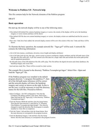
The example file is located in the directory "Pathloss 5examplesgislagos". Select Files - Open and
load the "lagos.gr5" file.
If the Pathloss program was installed in the default
program directory "c:program filespathloss 5", then
all of the full path name references will be correct
and the network display will show the backdrop
imagery and vectors as shown on the right. In this is
not the case, it will be necessary to reset the directory
names for the GIS files. Proceed as follows:
· Select Configure - Set GIS configuration. Note that the
Configure GIS dialog contains a file menu. Select Files -
Open and load the file "lagos.p5g" in the directory "Pathloss
5examplesgislagos".
· Click the Primary DEM tab and then click the Setup button.
Note that the main directory is specified as "C:Program
FilesPathloss 5examplesgislagosheight". This must be
changed to match the directory that the program is actually
installed in. Click OK on completion.
· Click the Clutter 1 tab and then click the Setup button. Rest
the main directory to correspond to the program location.
· Click the Backdrop imagery 1 tab and then click the Setup
button. Rest the main directory to correspond to the program location.
Page 1 of 53
3/10/2015
file://C:UsersaAppDataLocalTemp~hhEAAF.htm

· Click the Vector data tab and then click the Setup button. Rest the main directory to correspond to the program location.
· Save the GIS setup. Select Files - Save and save the file in the original location. Click OK to close the dialog. The Network
display will be reformatted to show the backdrop and vectors.
In the following descriptions of the basic operation, the example file can be used to illustrate the
concepts.
DRAFT
Navigating the network display
The first five buttons on the tool bar set the cursor mode which controls the network display
Pan cursor
Press the left mouse button and move the mouse to pan the network display. If the Ctrl key is
down then the operation changes to zoom as described below
Zoom cursor
Click the left or right mouse button to zoom or shrink the network display by 10%. The display
will be centered on the mouse cursor location. Alternately, left click and drag to zoom to the focus
rectangle extents. If the Ctrl key is held down, the operation changes to pan as described above.
Two additional buttons are used to zoom the network display. The 1:1 magnifying glass
button is only active when a backdrop image is present. The zoom level is set so that the
screen resolution is equal to the image resolution which is the optimum zoom for the image
resolution.
The extents button sets the zoom level to display the total drawing extents. This is determined by the
maximum of the site extents, image and vector extents.
Mouse wheel action
Rotate the mouse wheel forward or backwards to zoom in or out, This operates in any cursor mode and
has exactly the same effect as a left or right mouse button click in the zoom cursor mode.
Click the mouse wheel to enter the auto panning mode. The display panning direction and speed is
controlled by the mouse position, Left click to exit the auto panning mode
Link cursors
Link cursors are used to create links between sites and to access the link design sections.
Separate cursors are provided for point to point and point to multipoint links. These cursors are shown as
an arrow with sites attached to it - two sites for point to point and three sites for point to multipoint. The
only difference between these two cursors occurs when a link is created by a left click and drag between
two sites. The point to point cursor creates a point to point link. With the point to multipoint cursor, the
first site must be a base station to create a point to multipoint link
In the link cursor mode, hold down the shift key to temporarily switch to the pan
cursor. Hole down the Ctrl key to temporarily switch to the zoom cursor. With
Page 2 of 53
3/10/2015

these features and the mouse wheel operation, there should no need to change to
the pan or zoom cursors with the toolbar buttons.
In the link cursor mode, a left click on a site legend is used only to create new links by a click and drag
operation.
Right click on a site legend to access the site operations menu. These are described in Operations section
to follow
Left click on a link to access the design sections for that link. Note that only the
transmission analysis and terrain data selections will be active if the design
does not exist or a terrain profile is not available in the design
Right click on a link to access the link operations menu
Selection cursor
Network operations can be restricted to named
groups of sites / links. These groups are saved in the gr5
file. A selection is a temporary group and only one selection can exist at a time. The selection cursor
uses the standard windows arrow cursor. The operation is described below:
· Left click on a site to select it. Left click on a link to select the link and the sites at the ends of the link.
· Hold down the Ctrl key and left click on a site or link to add it to the selection or remove it from an existing selection.
· Click and drag to select the sites and links inside the focus rectangle
· Hold down the Ctrl key and click and drag to add the sites and links
· To clear a selection, click anywhere on the network display other than on a site or link
On screen measurements
Click and drag to measure the distance and azimuth between two points. The results can be copied.
Click Continue to make another measurement or click the check mark to end the measurements session
and return to the previous cursor mode.
DRAFT
Network display pictures
Pictures can be placed on the network display for presentation purposes. These can be in any of the
following image formats: bitmap, jpeg, gif or png. Click the picture button on the tool bar and click and
drag a rectangle to set the location of the picture. When the left button is released, an open file dialog
appears to open the required image file. While in the picture cursor mode, click on the picture and drag
Page 3 of 53
3/10/2015

to change the location or click on one of the corners and drag to change the size. Click on any other
cursor button to exit the picture cursor mode.
Select Backdrops - Pictures to edit the drawing order of the
pictures. The drawing order is top to bottom. The last picture in the
list will be on top of ay overlapping picture above this. Select a
picture file name and use the up and down arrows to change its
order in the list.
The erase button will delete a picture.
When a gr5 file is saved, the full path name of the pictures is save
in the file. When the file is loaded there is no error message if a
picture file is not found
DRAFT
On screen profile generation
A clutter data base is included in the Lagos.gr5 example. To enable this feature in this profile generation
example, select Configure - Set PL50L options - Terrain data - Profile generation and then select "Use
clutter 1 database.
Click the generate profile button. A profile preview window will appear. Position and size this window
as required. Click and drag to generate the profile. Note that clutter is not used on the profile preview.
On completion, the profile is regenerated to include the clutter and is presented in the antenna heights
design section of the PL50L link design program. The user can proceed to establish the feasibility of the
path and complete the design
If the profile starts on an existing site (the mouse cursor is inside a site legend when the click and drag is
initiated) then the coordinates of that site will be used. Similarly if the mouse cursor is inside a site
legend when the left mouse button is released, then the coordinates of the end site will be used.
Otherwise, the coordinates will be determined from the screen pixel location. Depending on the zoom
level, screen resolution, and the nature of the backdrop (geo referenced or edge referenced) inaccuracies
may result.
DRAFT
Elevation and clutter backdrops
Elevation and clutter backdrops are created for the current network display zoom level. The coordinates
of each pixel on the network display are determined and the elevation or clutter value is read from the
Page 4 of 53
3/10/2015

database. A bit map is created and displayed. If the display is subsequently zoomed, the bitmap is not
regenerated but simply zoomed to the new scale. These backdrops are therefore very dynamic. As the
network display view is changed to different areas, the user will regenerate the backdrop.
Two elevation backdrops are provided. The first button produces a display based only on the elevation
color ramp. The second button produces a shaded elevation. The third button produces the clutter
backdrop.
When an elevation or color backdrop is active the status bar shows the elevation and clutter type.
Elevation backdrop colors are set in the Backdrops - Elevation color ramp selection. Details of this
control are given in the general program operation section. The clutter colors are set in the GIS
configuration.
DRAFT
Extents - layers
Select the View - Extents-layers menu item. This dialog serves the following purposes:
· Shows the extents of each component of the network display and the composite extents. Any of these components can be
excluded from the composite extents
· allows the user to specify the extents of the network display. Click the Display button to show the extents of the current
network display. Note that this feature can be use on a new project which does not have imagery of vector data to define
the extents. The user would specify the extents and then create an elevation view to begin the project.
Page 5 of 53
3/10/2015

· Allows the user to selectively hide any of the network components. The toolbar buttons labelled B,
E, C and V, perform the same functions for the imagery backdrop, elevation and clutter backdrops
and vector data respectively.
· Sets the overall transparency of the elevation and clutter views and local and area studies. Note that
the transparencies of the individual colors can be set for elevation, local and area studies using the color ramp control. The
transparency cannot be set for the individual clutter colors
DRAFT
3D elevation view
The 3D terrain view provides an interactive view of the terrain, sites, links and fresnel zones in three
dimensions from any angle. The view uses the current elevation backdrop.
Create an elevation back drop for the area of interest and click the 3D display button on the tool bar. The
initial display shows the terrain viewed from above. Click the "Manual view" button to enter the
interactive display mode. The mouse movement, and the keys W, A, S, and D now control the
viewpoint. To exit this interactive mode, click the left mouse button.
· Moving the mouse forward or backward moves the view point ahead or back
· Move the mouse to the left or right to rotate the view point in that direction.
· The W key moves the view point ahead in the direction it is facing (zoom in)
· The S key moves the view point away in the direction it is facing (zoom out)
· The A key moves the view point to the left perpendicular to the direction that it
is facing (pan left)
· The D key moves the view point to the right perpendicular to the direction that
it is facing (pan right)
All of the keys and the mouse movement can be used
simultaneously to explore the display. Some dexterity and practice
is required. Experience with video games is an asset here.
Click the Reset viewpoint button to return to the initial display
3D Display
Toolbar
· The movement sensitivity slider controls the view point rate of change as the movement keys are pressed. Move the slider
to the left to decrease the rate and to the right to increase it.
· The display can include the following components:
terrain - draws all the ground and water.
Page 6 of 53
3/10/2015

Links - draws the links between sites as a straight line.
Sites - draws the actual tower at all site locations in the region.
Fresnel zone - draws the 3D Fresnel zones on all links
Fresnel grid - draws the 3D Fresnel zone as a grid of lines.
Orientation compass
· The "Copy" button copies the 3D display to the windows clipboard. It can be pasted into another program.
Settings
Click the Settings button to access additional
options for the 3D display. These settings can also
be accessed from the menu selection Configure -
PL50 program options - 3D terrain view. Note that
the link line width and vertical multiplier can be set
on the toolbar or in the program options. The
following options are available:
· Colors for link lines, Fresnel zones, Fresnel grids and site
towers
· link line width - the value is in relative units and has no
physical meaning. This number is used to create an
aesthetically pleasing and informative display. The number
can be set higher so the links can be viewed from a distance. It can be set to a low value to inspect links or Fresnel zone
intersections at close range.
· vertical multiplier - this exaggerates all the elevations in the 3D Display and is used to make mountain ranges or valleys
more prominent when viewing a large region.
· Fresnel zone reference (100% F1, 60% F1, 30% F1, F2, F4)
· Earth radius factor (K = 4/3, 1, 2/3 and infinity) - this will apply earth curvature to the terrain in the 3D Display. The terrain
will fall away on all sides from the center of the display The value of k determines the effective shape of earth to display.
Set K = infinity for flat earth.
Click on the green check mark when all the options are set as desired. The 3D display will be updated
automatically.
DRAFT
Groups and selections
Page 7 of 53
3/10/2015

Groups and selections of sites and links are used in all design operations. This is an essential feature
when working with large networks. A selection is temporary group which is created for a special
operation. Only one selection can be active at one time. Any number of groups of sites and links can be
created with individual names and these are saved with the gr5 file. Groups can overlap one another and
can be used to control the network display visibility.
Creating a selection
Click the selection button on the tool bar and create the selection using the methods below:
· click on a site or link to select it.
· hold the Ctrl key down and click on a site or link to add it to the selection -- or to remove it if it is already selected.
· click and drag to select a group of sites and links within the focus rectangle.
· hold the Ctrl key down and click and drag to add a group of sites and links to the selection.
To clear a selection, simply click anywhere on the network display other than on a site or link.
Creating groups
Select the Configure -- Group manager menu item to access the group manager dialog. To create a new
group, click the Add group button and enter a name for the new group. To add sites and links to the
group, just click on the sites and links to add or remove them from the group. In this mode, there is no
need to hold the Ctrl key down. You can also click and drag to add a group of sites and links.
The same procedure is used to edit an existing group. Set the current group in the drop down list and add
or delete the sites - links.
Add on Condition
Page 8 of 53
3/10/2015

Links can be added which meet certain conditions. At present the criteria are:
· path length
· frequency
· fade margin
Click the "Add on condition button, select the criteria and enter the range of values to be used to add the
group. Note that it is not necessary go enter values for both greater than and less than. For example, a
group of links with fade margins less than 15 dB, the greater than field would be left blank.
Edit as List
For advanced editing of group members,
click the Edit Group Members button.
This brings up another dialog box. The
group that you are editing is displayed at
the top. There are two list boxes that list
all the sites and links in the network.
Any sites or links that are in the group
will be highlighted in these lists.
Simply click on any site or link name to
add it or remove it from the working
group. You can click and drag down the
list to quickly select many sites or links.
Using Groups and Selections
An example of group operations is the
interference analysis. There are two drop
down lists labelled "Analyse [scope]
against [scope]
These `scope defining' items can be set to a selection, any group, all links or the master database. The
interference calculation will then be performed by testing only those sites in the Analyse group versus
only the sites in the against group. The members of the two scope groups can partially overlap,
completely overlap, or be totally distinct.
The network display will highlight the sites and links to show the scope. The first group will be
highlighted in blue, the second group will be highlighted in red. If part or all of the scope is overlapping,
those sites or links will be highlighted in purple.
Note: most operations work on either links or site, but not usually both. Groups can contain both sites
and links. When a group is chosen as a scope for some operation, only the correct members (sites or
links) are considered.
Creating Groups in the Site List and Link List
In the site list, select the sites to be added to the
group by left clicking in the first column. Hold
down the Shift or Ctrl key to multiselect the
Page 9 of 53
3/10/2015

sites. Then select the Create group menu item.
The sites can be added to a new group or an existing group.
The same procedure is used to add links to a group from the link list
Visibility of Groups
Click the Visibility button to show and hide groups.
All defined groups are shown in a list. If a group is
highlighted, its members will be displayed, if it is not
highlighted, its members may not be displayed.
There is also an option to hide or show sites and links
that do not belong to a group. For example, to display
a single group, check the "Hide ungrouped sites and
links" and then unselect every group in the list except
the one to be displayed.
Because sites and links may belong to multiple
groups the following rules determine if is a site is to
be shown:
· A site that is a member of any group marked as visible is
always visible.
· A site that is not a member of any group is hidden if the "Hide
Ungrouped Sites and Links" checkbox is checked.
· A site that is a member of one or more groups is hidden only if all of the groups of which it is a member are not visible.
(Corollary of first point)
Links follow the same rules as sites for visibility with one extra rule:
· If the site at either end of a link is hidden for any reason, the link will be hidden as well.
File operations
This section describes the procedures under the files menu and includes the export formats, moving
network files and operation with several people simultaneously accessing the network display gr5 file
Export to Shapefile
An ESRI shapefile actually consists of 3 different files. Two files (with extensions.shp and.shx) describe
the shapes themselves and another database file (.dbf) contains additional information about the vectors.
To export the network to a shapefile select Files - Export - Shapefile. You will be prompted for a file
name. This file name will be used for the three files that are created. Any extension you provide will be
ignored because shapefiles must have the expected extensions to function.
The links are stored as lines with end points in geographic coordinates referenced to the site datum.
Because a shapefile can only contain one type of shape, the sites are stored as lines as well except the
end points are the same and they have no length. The database file contains information about the sites
only. The following data is included: Site Name, Address, City, State, Country, Owner Code, Call Sign,
Page 10 of 53
3/10/2015

Station Code, Operator Code, Elevation, Tower Height, Latitude, and Longitude.
Export to Google Earth
This function creates a kml file from the network display. This file can be loaded in to Google Earth.
To export the network to Google Earth, select Files - Export - Google Earth kml. You will be prompted
to select which elements to export and then to choose a file name for the kml file.
If you included Sites and Links, they are included in the kml as points and lines.
If you selected Local Studies, image files will be created in the same directory as the kml file. There will
be one png image file for each local study. These image files are referenced as overlays in the kml file.
If the kml file is moved, these files must be moved to the same directory to be displayed.
If you selected Area Studies, a single image file is created for the area study and works in the same
fashion as local studies.
The studies in the kml use the current colors and criteria set in the color ramps for local and area studies.
The png format supports per-pixel transparency as does Google Earth.
To load the kml file in Google Earth simply select Files - Open and browse to the kml file. Google Earth
should automatically fly to the area.
DRAFT
Link design
Page 11 of 53
3/10/2015

The link design dialog is used to set the design rules, calculation methods, algorithms and all equipment
parameters in point to point and point to multipoint applications.
Note that the dialog contains a Files menu and a Set PL50L option menu selection. The design
specifications are saved in a link design file with the suffix ld5. Access to the PL50L options is
necessary to select the basic application and algorithms.
The differences between point to point and point to multipint applications are given below:
· The "Antenna heights - TX lines" options requires a fixed height for the base station in a point to mulitpoint application. In
the point to point version, the antenna heights at both ends of the path can be calculated.
· In a point to point application, the equipment parameters are specified and saved in the ld5 file. In a point to multipoint
application, the equipment parameters are considered to be part of the base stations and are saved in the gr5 file.
The example on the right is for a point to point link design as used in the transmission analysis design
section for a single link. In the network display, the link design dialog is the core of the following
operations:
· create point to point links
· create point to multipint links
· design point to point links
Page 12 of 53
3/10/2015

· design point to multipint links
DRAFT
Design scope
The design scope options depend on the specific operation required.
Generate terrain profile
A terrain database must be configured for this operation. If a path profile exists, it will be automatically
overwritten if the profile has been flagged as invalid. If the profile has been modified, the user will be
prompted to change the profile.
Calculate / assign antenna heights
If this option is not checked, the existing antenna heights will be used; otherwise, the antenna heights
will be set as specified in the "Antenna heights - TX lines" dialog below.
Add data
separate options are provided for antenna, transmission lines, antenna coupling unit and radio
equipment. On a new link design all of these would be applicable; however, the operation could also
involve only a change of radio equipment
DRAFT
Point to point antenna heights - TX lines
Antenna height calculation
If the point to point link design is
being used to determine network
connectivity, then the antenna
height calculation method will
depend on the rejection criteria.
If the rejection criteria is antenna
height, then do not check the "Limit
antenna heights to the maximum
specified values".
If the rejection criteria is diffraction
loss, the "Limit antenna heights to
the maximum specified values"
must be checked.
Unless fixed heights are used at site
1 and site 2, the antenna heights
will be calculated using the
specified clearance criteria
Page 13 of 53
3/10/2015

Transmission line length
Several options are provided to specify the transmission line length, The transmission line unit loss is
specified under the equipment specifications section
DRAFT
Point to multipoint antenna heights - TX lines
Antenna height calculation
Click the Antenna heights button on the Link design dialog. The hub sight antenna height must be set in
point to multipoint applications.
If the operation is to create PTMP links and determine their feasibility, the antenna height calculation
method will depend on the rejection criteria.
If the rejection criteria is antenna height, then do not check the "Limit remote antenna heights to the
maximum specified value".
If the rejection criteria is diffraction loss, the "Limit remote antenna heights to the maximum specified
value" must be checked and this maximum value specified.
The remote antenna heights will be calculated using the specified clearance criteria, unless a remote
fixed height has been specified.
Transmission line length
Page 14 of 53
3/10/2015

Several options are provided to specify the transmission line length, The transmission line unit loss is
specified under the equipment specifications section
Antenna coupling unit
Click the Antenna coupling unit button in the Link design dialog. The specific format of the data entry
form will depend on the application (microwave, adaptive modulation or land mobile.
DRAFT
Point to point equipment specifications
Click the Equipment specifications button in
the Link design dialog. Antenna, transmission
lines and radio equipment are specified here.
Data can be added by either using a template
file or the standard equipment index files.
Click the blue button opposite the equipment
type to access that index file.
A template file is any pl5 file which has the
required equipment specifications. Click the
template file button and open the pl5 file.
DRAFT
Point to multipoint equipment specifications
Page 15 of 53
3/10/2015

Click the Equipment specifications button in the Link design dialog. The equipment specifications in
point to multipoint systems are part of the base station. This data is saved with the base station in the gr5
file. Note that in the case of point to point equipment specifications, the data is saved in the link design
ld5 file. The point to multipoint dialog is organized into the following sections:
Hub (base station) sector antenna - radio data
Always do the data entry for sector 1. When sector 2 is initially selected, the data from sector 1 will be
copied into sector 2. Manual data entry can be used for single sector omnidirectional antenna. In this
case there will be no adjustment for vertical angles. Click the blue button for the base antenna code to
access the antenna index. An antenna code is required for interference calculations and for multi sector
antenna arrangements.
Manual data entry is adequate for coverage analysis. A radio code is required for interference analysis.
Click the blue button for the base radio code to access the radio index.
Set the polarization and the channel id for an interference analysis.
Sector definition
Page 16 of 53
3/10/2015

A maximum of 8 sectors can be specified. The specific sector number to be displayed is set here.
symmetrical sectors - if this selection is checked, only the azimuth of sector 1 can be edited. The
program will calculate the azimuth for the other sectors. If this is unchecked all sectors azimuths can be
edited
Provision is made to set the same antenna and radio data and polarization in all sectors. Click the click
the corresponding blue button
For interference analysis, click the blue button to load the frequency plan and identify the base station or
remote site as the high frequency site.
Mobile (remote) antenna - radio data
Manual data entry can be used for the remote antenna. In this case there will be no adjustment for
vertical angles. Click the blue button for the remote code to access the antenna index. An antenna code
is required for interference calculations.
Manual data entry is adequate for coverage analysis. A radio code is required for interference analysis.
Click the blue button for the remote radio code to access the radio index.
Transmission lines
If transmission line lengths have been specified for the base or remote antenna in the Antenna heights
and transmission line lengths section, then click the blue button corresponding to that transmission line
and select the transmission line. The transmission line data can also be entered manually.
Duplex and multiple access technology
The calculation of the composite interfering signal depends on the duplex and multiple access
technology used in the radios. The duplex technology can be frequency or time division duplex -
synchronized or non synchronized.
The multiple access technology can be frequency division multiple access, time division multiple access,
code division multiple access or OFDMA.
DRAFT
Reliability parameters
The format will depend on the current multipath fade probability algorithm. Remember that this can be
changed by selecting the Set PL50L options menu item. The dialog for each algorithm is shown below.
The data entry requirements are self explanatory and are described in the transmission analysis section.
Page 17 of 53
3/10/2015

of 53
3/10/2015

DRAFT
Rain parameters
The format will depend on the current rain algorithm setting - Crane or ITU530. Remember that this can
be changed by selecting the Set PL50L options menu item. The dialog for each algorithm is shown
below
Network
operations
This section
describes the
operations
under the
Operations
menu in the
network
display.
Many of
these
operations
use groups
and selections and the Basic operation section of the
documentation is a prerequisite to this section.
DRAFT
Add site on screen
Select Configure - Add site to access the Add SIte dialog. The add site cursor will appear on the network
display. Position the cursor and click the Add button to create a new site at the cursor location. If the
"auto name sites" option is checked, the site name will be created using the format specification show
Page 19 of 53
3/10/2015

and the new site will be automatically entered into the site list and shown on the network display.
If auto site naming is not used, then an intermediate data entry
form will appear with all of the available site data fields
Note that the site coordinates are calculated from the screen
pixel location. Depending on the zoom level, screen resolution,
and the nature of the backdrop (geo referenced or edge
referenced) inaccuracies may result.
Move site on screen
Invoke the Move Site dialog by either of the following means:
 Right click on the site legend and select move site
 Select Operation - Move site and then left click on the site legend to identify the site to move
Click on the display to position the move site cursor and then click the OK button to move the site. This
procedure will invalidate any path profiles associated with the new site location.
Note that the site coordinates are calculated from the screen pixel location. Depending on the zoom
level, screen resolution, and the nature of the backdrop (geo referenced or edge referenced) inaccuracies
may result.
DRAFT
Create point to point links
This procedure uses the point to point link design
rules to determine the best overall connectivity
for a group of sites and to complete the link
design for the final configuration.
The following combinations of sites can be used
Page 20 of 53
3/10/2015

for the analysis:
· from all sites to all sites.
· from one named group to another named group
· from a selection to a named group
· from all sites to all sites in a selection
There are practical limitations for the total number of links that can analysed. For example a network of
100 sites would generate n*(n-1)/2 = 4950 links using the all sites to all sites combination
Create the required group(s) - selections for the analysis and select Operations - Create point to point
links.
Click the Link design button and set the design rules and parameters.
Click the Display criteria button and
select the display criteria and the
associated color legend. Currently the
available display criteria are antenna
height, diffraction and fade margin. Note
that for antenna height and diffraction, the
equipment specifications are not
necessary.
Refer to the general program operation
section for setting up the color ramp. Any
number of ranges can be specified;
however, as only the link lines will be
colored, choose distinctive colors for each
range.
Click the Create links button. The links
will be created and color coded according
to the display criteria settings.
Click on a specific link to view the
parameters
Specify the rejection criteria. Leave any
unused criteria blank. Click reject links to
hide the rejected links.
Page 21 of 53
3/10/2015

Once the final link configuration is determined. Click
finalize links to create pl5 files for the links and register
these on the display.
DRAFT
Create point to multipoint links
This
procedure
uses
the
point
to
multipoint
point
link
design
rules
to
create
links
from
a
base station to a defined set of remote sites. The links can be rejected based on path length, remote
antenna heights, diffraction loss or fade margin.
There are several ways to control the number of remote stations to be connected:
· create a selection of the remote stations
· create a group of remote stations
· specify a radius from the base station.
The first two methods must be completed before starting the procedure.
Page 22 of 53
3/10/2015

Right click on the site legend of the central site and select the "create PTMP links" menu item. This site
will become a base station.
Select the link sites method to either the
group or selection or to sites within the
specified radius. In the first case select the
group or selection. In the second case
enter the radius or click the blue button
and then click on the network display to
specify the radius.
Click the Link design button and set the
design rules and parameters. If sectorized
antennas will be used, these should be
specified at this time. The design
procedure will assign each remote to the
best sector and will take the sector
antenna pattern, azimuth and elevation
angle into account.
Click the Display criteria button and
select the display criteria and the
associated color legend. Currently the
available display criteria are antenna
height, diffraction and fade margin. Note
that for antenna height and diffraction, the
equipment specifications are not
necessary.
Refer to the general program operation
section for setting up the color ramp. Any number of ranges can be specified; however, as only the link
lines will be colored, choose distinctive colors for each range.
Click the Create links button. The links will be created and color coded according to the display criteria
settings.
Click on a specific link to view the parameters. Specify the rejection criteria. Leave any unused criteria
blank. Click reject links to hide the rejected links.
Page 23 of 53
3/10/2015

Once the final link configuration is determined. Click
finalize links to create pl5 files for the links and register
these on the display.
DRAFT
Design links
The design links feature operates on the following:
· a named group or selection consisting of point to point links.
· a name group or selection consiting of point to multipoint links connected to the same base station.
Page 24 of 53
3/10/2015

The links can be new links or existing links with pl5 file associations. The link desing will be saved in
the pl5 file.
Select Operations - Design links to access the design links dialog.
The Link design dialog is used to set the design rules and parameters. Click the Design criteria button to
access this dialog.
Check the required file naming convention and click the Design links button to carry out the design.
Frequency assignments
A pl5 file contains the channel frequency and polarization assignments. These are set in the transmission
analysis section on a link by link basis. The frequency assignment utility allows these assignments to
made in the network display.
Create a selection or a named group of the links requiring frequency assignments. Each link must have a
pl5 file association. Select Operations - Frequency assignments. Select the required group or selection.
Only the selected group or selection will be displayed.
The default frequency plan (the last used frequency plan) is initially loaded. If required, click the "Open
frequency plan file" button and load the required file. Set the channel number to be used in the
assignments.
The first step is to identify the high frequency sites. Click the "Identify high frequency site(s)" button.
Click on the site legend of a high frequency site. All links connected to this site will be automatically set
Page 25 of 53
3/10/2015

based on the site initial designated as high. Repeat this high frequency site assignment for any
unconnected links.
The "Reset all high - low designations" simply resets all sites to the undefined high - low state.
Two buttons are provided for polarization assignments. The "Set all polarizations to vertical" resets all
links to vertical. The link polarization is show as a label on the link lines. Click the "Toggle polarization
H<->V" button. Then click on a link to change its polarization.
At this point the selected channel number and polarization can be assigned to all sites. Click the "Add
new channel assignment" button. To add additional channel assignment, select the new channel number,
change the polarizations if required and click the "Add new channel assignment" button again.
The "Clear all channel assignments" will erase the TX channel records in the pl5 files for all links
The TX channel tables of the individual links can be directly edited in the network display. Click the
"Edit channel assignments" button. Then click on a link to edit the channel table
DRAFT
Performance reports
The performance - objective report feature
uses a named group of links. The normal
"All links" or a selection cannot be used.
The order of the links and the direction can
be edited and this is saved as part of the
group. Create the group of links for the
performance report and select Operations -
performance.
The initial display shows the list of the
available groups and the link members in
each group. The buttons on the right side of
the display are used to set the order of the
links and the direction as they will appear in
the report.
Click
the
Objectives
button
and
if
necessary
select
the
calculation
method
and
Page 26 of 53
3/10/2015

enter
the performance objectives. Note that if the specific objectives are not entered, then the report will only
show the calculated performance.
The objectives can be referenced to the total length of the selected links or to a hypothetical reference
path. In the latter case the reference length in kilometers is required.
Click the OK button on completion of the objective settings and click the report button on the initial
display to generate the report.
DRAFT
Site coordinates datum
Two utilities are provided to deal with datum discrepancies between the network display GIS settings
and the associated pl5 files.
Transform site coordinates
Select Operations - Transform coordinates. The "To datum" is fixed and represents the datum specified
for the site coordinates tab in the GIS setup.
Set the "From datum" to correspond to the site coordinates that require transformation. In most cases,
the coordinates in the associated pl5 file will also need to be changed.
Set pl5 files datum projection.
Page 27 of 53
3/10/2015

This utility simply changes the datum and projection in a group / selection of pl5 files. The datum will
be changed to that specified for the site coordinates tab in the GIS setup. Several recalculation methods
are also provided if a projection is used.
DRAFT
Thematic mapping
The default site and link attributes offer a limited selection of shapes and line styles to differentiate
between different classes of site and links. These attributes are described in first part of this section. The
second part deals with thematic mapping of sites and links which includes the capability of coloring the
legends according to their status
Site attributes
Select PL50 program options -
Attributes - Site name - legend. The
following default attributes can be set
for the site legend:
· color
· shape (circle, square or triangle)
· solid fill or outline
· size expressed in millimeters
Existing sites in the network display can
be reset to any or all of these attributes.
These attributes will be assigned to all
new sites.
The following default attributes can be
Page 28 of 53
3/10/2015

set for the site name label.
· base font, font style (bold or italic), color and point size
· the name label can include the site name, call sign, coordinates and the elevation.
· the "default positions" button sets the site name label position relative to the site legend to the initial default location.
To set the attributes of a particular site,
right click on the site legend or site
name.
On dense networks the display can be
more readable when the site name label
is switched off. To view the name or
turn the label back on, right click on
the site legend.
To set the position of the site name
label, left click on the label and drag it
to the new location
Link
Attributes
Select
PL50
program
options -
Attributes
- Link
lines.
The
following
default attributes can be set for link lines:
· color
· line style (solid, dash or dot)
· line width
Existing links in the network display can be reset to any or all of these attributes. These attributes will be
assigned to all new links
To set the attributes of a particular link, right click on the link
and select site legend or site name. The same attributes are
available as in the default link attributes above
Link
Labels
Select
PL50
Page 29 of 53
3/10/2015

program
options - Attributes - Link labels to set the default link label or right click on a link and select Link label
to set the label for a specific link.
Label format
A label can either have a fixed free format or can be one of the predefined formats. In the latter case, the
label data will be taken from the pl5 file associated with the link. If a file association does not exist, the
label will not be drawn. The following label formats are available:
· TX frequency and polarization
· TX channel ID and polarization
· distance and azimuth
Link labels use the site name font
Link Attributes
Link labels use the site font. The font style (bold, italic), color and the point size can be set.
If the shrink to fit option is checked, the label drawing will start at the specified point size and if
necessary the point size will be reduced until the label fits on the link line.
Label drawing can be suspended by checking the "Do not draw" option
Labels can be drawn above or below the link line.
The "Update Labels" button in the default link label options will reread the label data from the
associated pl5 files.
Site Thematic Legends
True type fonts are used for the site legends in thematic mapping The webdings and wingdings fonts
contain characters which are suitable for this purpose. There are two parts to a thematic site legend. The
site type determines the symbol and the site status determines the color. At present, 8 site types and 8
site status values are available.
If both site type and site status are undefined then the standard circle, square and triangle shapes are
used. If the site type is defined and the site status is not defined, then the font can be edited using any
combination of colors.
Click the "site list" tool bar button or select the View - Site list menu. The thematic site legend columns
are Site type and Site status. These are both drop down lists include a "not specified - defined" item and
the 8 site and status types.
Site Type
Select the "Thematic
mapping - Site type" menu
Page 30 of 53
3/10/2015

Place the marker on the
symbol cell for the site number being defined and click Enter or double click on the cell. Each time a
symbol is defined, it will be added to a list of symbols. This list is automatically saved in the
file..cstmdatathsymbol.lst.
Click the New button to create a new symbol. Click the Font
menu and choose a font. Double click on a character to select it.
If the site status will not be used,
then click the edit button and set
the colors as desired
Enter a name for the site type (the
default names are "Type 1 to 8), set
the active state and the point size
of the legend
Site Status
Select the "Thematic mapping -
Site status" menu
Enter a name for the status, set the
active state and double click on the
color column to set the color.
In the site list double click on the
Site type cell or Site status cell to
set the particular value
Thematic links
Click the link list button on the toolbar or select the View - Link list menu.
A thematic link line consists of three components. The link type and link status are equivalent to the site
type and status described above. The link type determines the line style and the link status determines
the line color. The third component is actually a second link line whose style and color represent another
status variable for the link. The expected use of this second links line is to track the line of sight testing
on large metropolitan networks. This status is designated LoS
At present, 8 link types and 8 link status and 8 LoS status values are available.
Page 31 of 53
3/10/2015

If both link type and link status are undefined then the standard solid, dash dot lines defined under link
line attributes are used. If the link type is defined and the link status is not defined, then the line color set
in the line type definition is used.
Note that the Los line (second link line) is drawn first. The link status line is drawn on top of the LoS
line. The line styles, widths and colors should be chosen, so that both lines are visible.
The thematic link line columns are Link type, Link status and Line of sight (LoS) status. These are both
drop down lists include a "not specified - defined" item and the 8 link, status and LoS states.
Link type
Select the "Thematic mapping - Link type" menu. Enter a name for the link type (the default names are
Page 32 of 53
3/10/2015

"Type 1 to 8) and set the active state.
To set the line style, double click on the line style cell. Choose one of the Windows standard line styles
or create a saw tooth, square wave or sine wave line. If the link status is not defined, the line color can
be specified; otherwise the link status color will be used.
Link status
Select the "Thematic mapping - Link status" menu
Enter a name for the status, set the active state and double click on the color column to set the color.
Line of sight status
Select the "Thematic mapping - LOS status" menu
Enter a name for the LOS status and set the active state.
Double click on the line style cell. Choose one of the Windows standard line styles or create a saw tooth,
square wave or sine wave line. Both the LOS status and the Link type lines are displayed.
DRAFT
Overview
Intra system interference is calculated in the Network module. The calculation considers only the
displayed layers. All sites and links which are not on an active layer will be ignored. The calculations
use antenna and radio codes. An antenna or radio code is the data file name without an extension. These
contain the parameters required for an interference calculation and are described in detail in this section.
The minimum conditions to calculate intra system interference are listed below:
· A Pathloss data file (pl4 or pl5) must be associated with each link to be used in the calculation.
· An antenna code must be specified for each antenna in the Pathloss data file.
· The transmission analysis must be complete to the level of a receive signal calculation.
· Transmit and receive frequency assignments must be specified for the Pathloss data files used in the calculation.
A radio code is optional; however, only the interfering level will be calculated without this file. A radio
code is required to calculate filter improvement and threshold degradation.
Note that there is no provision to calculate the interference from a transmitter into a receiver located at
the same site.
On completion of an interference calculation, the user is prompted to save the calculation results. The
default file name is the gr5 file name with the extension ifr. The file can be reloaded provided that the
current gr5 file was used to create the interference file or the network display is blank.
DRAFT
Interference calculation procedure
Page 33 of 53
3/10/2015

Select Interference - Calculate Interference from the Network display menu bar. The "Intra System
Interference" dialog box sets the options for the calculation.
Study scope
Interference is calculated between two sets of links. One set of links can act as the interfering
transmitters and the other as the victim receivers or both sets can act as interfering transmitters. These
sets of links can be a selection, a named group of links, all links or the master data base.
Select the two sets of sites and click on the green arrow to change between a single direction and
bidirectional analysis. Note that if the two sets are the same, then the calculation is inherently
bidirectional and the specified direction has no effect.
When analysing one set of links against second set of links, it is expected, that the user will define two
independent sets without any overlapping links. If there are overlapping links an intra system calculation
will be carried out in the overlap area will be carried out and this can result in duplicate interference
cases. These duplicates are removed from the results; however, as a cautionary measure, the user is
advised to examine the cross reference report to verify that duplicates are not present.
When an interference analysis between the network display and the master data base is carried out,
duplicate interference cases can also occur. In this case, the test for duplicate interference cases can be
ambiguous and the user is responsible to delete any duplicates.
Digital interference objective
The objective is specified in terms of the allowable receiver threshold degradation. For frequency
coordination with other operators, the usual value is 1 dB; however, for intra system interference, the
final criteria is determined by the increased outage times resulting from the actual threshold degradation.
Note that the allowable threshold degradation determines the composite interfering level. A calculation
Page 34 of 53
3/10/2015

margin described below is subtracted from this composite interfering level to established a reporting
threshold level. The following example illustrates this procedure.
threshold degradation 1 dB - user specified
receiver noise floor -107 dBm - calculated from RX threshold data
interfering level -113 dBm - calculated from receiver noise floor and threshold degradation
calculation margin 10 dB - user specified
reporting threshold -123 dBm - all interfering signals below this level will be ignored
Sometimes an analysis shows that there are no interference cases and the user would like to examine all
interference calculations. This can be accomplished by lowering the reporting threshold using a
threshold degradation of 0.01 dB and a calculation margin of 200 dB. In the above example, these values
would result in a reporting threshold of -333.5 dBm which will show all cases in any practical system
Default Minimum Interference Level
In the above reporting threshold example, the interfering level required to meet the threshold
degradation objective was calculated from the receiver noise floor. In the event that the receiver noise
floor is not available, the default minimum interference level will be used as the interfering level
required to meet the threshold degradation objective. The reporting threshold level will then be given by
the default minimum interference level minus the calculation margin.
Calculation Margin
The calculation margin sets a tolerance on the reporting of interference cases. If the interference level
objective for the receiver under test is -104 dBm and the calculation margin is set to 10 dB, then all
interference cases greater than -114 dBm (-104 - 10) will be reported.
The threshold degradation objective will be converted to an interference level objective for each receiver
in the calculation.
Coordination Distance
Interference is not calculated if the interfering path length is greater than the specified coordination
distance.
Maximum Frequency Separation
Interference is not calculated if the difference between the interfering transmitter and victim receiver
frequencies is greater than the specified maximum value.
Note that if a radio data file is not available, a cochannel interference analysis can be carried out by
setting the maximum frequency separation to some value less than the TX to RX frequency spacing.
Ignore Diversity Antennas
This option ignores all receive frequencies associated with a space diversity receive only antenna. In the
initial frequency analysis, this option will reduce the number of cases by 50%. If the main and diversity
antenna gains are different, then the final analysis should consider the diversity antennas.
Ignore Adjacent Channels
Page 35 of 53
3/10/2015

This option applies to 1 for N systems. Once the threshold degradation of the adjacent channels has been
established, use this option to limit the number of interference cases.
Calculate OHLOSS automatically
This option will automatically calculate the over the horizon loss (OHLOSS) on all interfering paths
which do not have a direct link to the affected receiver. Click the OHLOSS option button to set the
specific options for the OHLOSS calculation.
OHLOSS calculations can be a contentious item when resolving interference case between different
organizations It is important to note that if an OHLOSS calculation results in a interfering level below
the reporting threshold, the interference case will not appear in any report. If the OHLOSS calculations
are carried out in the case detail report screen after the main calculation is complete, the OHLOSS cases
will remain in the analysis.
OHLOSS options
Click the OHLOSS options button in the Intra system interference dialog. These options will be used in
all OHLOSS calculations in the present analysis. Refer to the help in the diffraction loss section of the
PL50L program for complete details on the OHLOSS calculation procedure.
An OHLOSS calculation takes time variability into account. Current practice is to compute a long term
and a short term time variability. The long term is normally set to 80%. Threshold degradation
objectives refer to this long term objective. In the short term, the allowable threshold degradation can be
significantly higher.
If required set the diffraction algorithm, the climatic region and the short and long term time
percentages.
DRAFT
Correlation options
Page 36 of 53
3/10/2015

When an interference path is the same as the main path, the interference case is defined as correlated. In
this case it is expected that fading on the interfering main paths will occur at the same time. In the case
of multipath fading, the actual fade depths on the two paths will depend on the type of correlation. If the
interfering transmitter antenna heights are the same as the main transmitter heights, then the two paths
are completely correlated. In this case it is common practice to ignore the case, particularly if automatic
transmit power control is employed. The main path will increase power in response to the fade; however
the interfering transmitter may not change.
A partially correlated situation exists when the interfering transmitter antenna heights are different than
the main transmitter antenna height. In this case, an additional loss in the order of 5 to 10 dB is added to
the interfering signal
Although the same correlation options are used for both mulipath and rain, the definition of correlation
is actually whether the interfering and main paths are in the same rain cell.
Click the Correlation options button in the Intra system interference dialog to set the correlation options
DRAFT
Interference calculation
The calculation starts by building transmitter and receiver tables for the two sets of links. If the two sets
are the same, then only one set of transmitter and receiver tables is required.
If the integrated PL50L program is running with one of the required links, the transmit and receive data
is taken from the PL50L data; otherwise, the data is read from the Pathloss data file associated with each
link. The Pathloss data file in memory can be edited and when the interference is recalculated to see the
effects of the changes.
Interfering level objective
The interfering level objective Iobj is calculated for each receiver as follows:
(1)
where:
Page 37 of 53
3/10/2015

T
do
allowable threshold degradation specified in the Interference dialog box.
N
rx
receiver noise threshold in dBm
The receiver noise threshold calculation will depend on the specific data available in the radio data file
Threshold to Interference T_I and the 10
-6
BER receiver threshold RXthr
Nrx = RXthr -- T_I + 5.868 dBm
3 dB carrier to interference C_I3dB measured at the 10
-6
BER receiver threshold RXthr10^6
Nrx = RXthr10^6 - C_I3dB
3 dB carrier to interference C_I3dB measured at the 10
-3
BER receiver threshold RXthr10^3
Nrx = RXthr10^3 - C_I3dB dBm
Receiver noise figure NF and 3 dB receiver bandwidth BW3dB
Nrx = 10 * log10(n_f) + 30. + NF dBm
where
n_f = K * T * BW
3dB
* 1.E6
K 1.380658E-23 (Boltzman's constant)
T 290 degrees Kelvin
and the 3 dB bandwidth is expressed in MHz
This interfering level objective represents the total power in the victim receiver passband which will
degrade the receiver threshold by the specified amount. At this point, the frequencies and the
bandwidths of the interfering transmitter and victim receiver are not considered. These will be used later
to calculate the filter improvement.
If the receiver noise threshold is not available due to missing data, the default minimum interfering level
will be used as the objective.
Note that Iobj - calculation margin is the reporting threshold.
Interference case rejection
As the calculation proceeds, an interference case will be rejected at any point if its interfering level is
less than the reporting threshold, Several other conditions to reject an interference case are as follows:
· The difference between the transmitter and receiver frequencies is greater than the specified maximum.
· The transmitter is located at the same station as the receiver.
Page 38 of 53
3/10/2015

· The transmitter is associated with the receiver under test.
· The interfering path length is greater than the specified coordination distance. The path length is calculated from the receive
and transmit coordinates.
Free Space Loss Interfering Signal
The free space loss interfering signal level is calculated as follows:
Ifs = TX power + TX antenna gain + RX antenna gain - TX loss - RX loss - free space loss.
Antenna Discrimination
The effects of the transmit and receive antenna discriminations are now considered:
· Calculate the antenna discrimination angles for the TX and RX antennas.
· Calculate the antenna discrimination for the TX and RX antennas. This calculation uses the antenna data files.
· Calculate the interfering signal levels for all combinations of TX and RX antenna polarizations.
Antenna discrimination is characterized by the four polarization combinations HH, HV, VV, and VH.
The first letter is the polarization of the antenna under test. The second letter is the polarization of the
signal being received or transmitted. For example, the term HV is the response of a horizontally
polarized antenna to a vertically polarized signal.
At first glance, the total antenna discrimination would be obtained by adding the appropriate
polarization combinations of the interfering transmit antenna and the victim receiver antenna.
Unfortunately, this is not the case, as the ratio of horizontal and vertical polarized signals is unknown.
The following polarization combinations are determined and the minimum value is assigned as the total
antenna discrimination:
Tx H Rx H (HH) HH HH
HV HV
Tx H Rx V (HV) HV VV
HH VH
Tx V Rx V (VV) VV VV
VH VH
Tx V Rx H (VH) VH HH
VV HV
An example of this analysis is given below for a free space loss interfering signal level of -38.59 dBm.
The first letter in the polarization combination is the transmit polarization; the second letter is the
receive polarization.
Page 39 of 53
3/10/2015

Antenna Discrimination HH HV VV VH
Interfering TX 0.00 32.00 0.00 32.00
Victim RX 65.00 69.00 67.00 69.00
Total Discrimination (dB) 65.00 69.00 67.00 69.00
Interfering Signal (dBm) -103.59 -107.59 -105.59 -107.59
If the interfering level for the specified polarization is less than (Iobj - calculation margin), then the
interference case is rejected.
If this is a cochannel case (same transmit and receive frequencies) and the same radio codes are used for
the transmitter and receiver, the calculation for this interference case is complete.
Filter Improvement
Radio data files are required to calculate the filter
improvement. If a radio data file does not exist for
the victim receiver, the calculation terminates. The
calculation sequence for filter improvement proceed with the following steps.
· If the transmitter modulation is designated as "Analog", the filter improvement will be interpolated from the receive radio
code receiver selectivity curve.
· If the receiver and transmitter codes are the same and the code file contains a TtoI_Same curve or an IRF_Same curve, the
filter improvement will be interpolated from this curve.
· if the receiver code file contains an TtoI_Other curve or an IRF_Other curve for the transmit radio code, the filter
improvement will be interpolated from this curve.
If the required T to I or interference reduction factor curve is not available, the filter improvement will
be calculated by convoluting the spectrum of the interfering transmitter against the victim receiver
selectivity. There are two levels of default for both the transmitter and receiver.
If the transmitter radio data file includes a measured transmit spectrum, this will be used; otherwise, the
default emission mask is used. In both cases, the data is normalized, so that the area under the curve is
unity as shown in Equation (2).
(2)
where PI(f) is the power spectral density of the interfering transmitter. This normalization
was carried out when the radio data file was created from the ASCII version
The receiver selectivity calculation curve
(RX_SELECTIVITY_CALC) is generated when
the radio data file is created using the following
priorities for the source data:
· user receiver selectivity data. This must represent the
composite receiver selectivity curve and include the RF,
IF, and baseband (Nyquist) filtering
Page 40 of 53
3/10/2015

· T to I curve for a carrier wave modulated (CW) interferer
· default receiver selectivity mask
This curve is optimized for the convolution process by using a variable point density concentrated
around the receiver passband.
The receiver selectivity and interfering power spectral density are convoluted together to calculate the
filter improvement FI as follows:
(3)
where:
f interfering frequency - receiver frequency
H
r
(f) receiver selectivity (RX_SELECTIVITY_CALC curve)
P
i
(f) power spectral density of the interfering transmitter
Threshold Degradation
The threshold degradation is calculated using the following formula.
(4)
where
Td threshold degradation (dB)
Nrx receiver noise threshold (dBm)
Ifl interfering signal level (dBm)
The composite threshold degradation is calculated in the same manner using the power sum of all
interfering signals.
DRAFT
Fade correlation
Page 41 of 53
3/10/2015

Once the basic interference calculation has been completed, the rain and multipath fade correlation can
be set for each interference case. Select Interference - Fade correlation on the network display menu bar.
Step through the cases and sub cases to view the interference cases.
Use the go to case button to set a specific case number. on the cross reference report
The current interference case - sub case is shown on the network display
The following abbreviations are used in the display:
itx interfering transmitter antenna height
arx adjacent transmitter antenna height
v-i victim receiver to interfering transmitter distance
ang receive antenna discrimination angle
ifl interfering signal level
td threshold degradation
Refer to the Fade correlation options section for details of the concept and typical values for fade
correlation
Overview
These studies calculate the signal strength from a base station over a user defined area. This area is
divided into square cells and a calculation is made for each cell to form the overall display. In a local
study the area is a circle with its center at the base station. The user specifies the radius to define the
area. All calculations in a local study are limited to this circle around the base station. A composite local
study display from a number of base stations with overlapping coverage areas can be produced. This is
drawn using the strongest signal from each base station.
Page 42 of 53
3/10/2015

An area study shape can be a rectangle, ellipse of an irregular polygon. This shape can be positioned
anywhere on the network display. The area is divided into square cells as in the case of the local study;
however the calculations for each cell can be made for multiple base stations. In addition to signal
strength, the following additional analysis can be carried out:
 most likely server
 carrier to interference
 simulcast delay spread
Terrain database usage
A calculation starts with a terrain profile from the base station to the cell under test. This depends on the
specific GIS configuration and the terrain database usage settings. Select Configure - PL50L program
options - Terrain data - Profile generation to set these options. Normally the program detects changes to
the parameters with affect the calculations such as antenna heights or display criteria. In the case of
changes to the GIS configuration or the usage options, a "forced recalculation" option is available which
will completely redo the calculation. It is expected that some experimentation will be required with
clutter database which necessitates a recalculation.
DRAFT
Clutter loss calculations
Clutter data bases fall into two categories:
· The database contains only the elevation of the clutter. No other information is available
· The database contains a description of the clutter. The user assign heights to each clutter type and specifies a creates a cross
reference to a set of standard clutter categories. These standard categories in turn define the clutter loss versus frequency
and the standard deviation of the log normal probability distribution used to calculate location variability.
In the first case, the clutter heights are added to the terrain profile. The diffraction loss calculation first
calculates the loss due to terrain only and then the additional loss due to the clutter heights. The user
specifies a default clutter category which in turn sets the log normal standard deviation for location
variability. This correction is applied to all cells.
In the second case, the clutter heights are added to the terrain profile, however there is 200 meter
exclusion zone at the end of the profile with no clutter heights. The diffraction loss calculation first
calculates the loss due to terrain only and then the additional loss due to the clutter heights taking into
account the exclusion zone. The clutter category for the cell determines the clutter loss to be added and
Page 43 of 53
3/10/2015

the log normal standard deviation. The additional losses provided by the clutter database area
summarized as follows:
· Clutter heights along the terrain profile produces additional loss to the terrain only calculation. This loss depends on the
both the assigned heights of the clutter the type of clutter.
· The clutter category includes a table of loss versus frequency to account for the effects of clutter in the immediate vicinity
of the receiver. This is added to the calculation
· The clutter category also includes the log normal standard deviation. For location variability time percentages greater than
50%, an additional loss is added to the calculation to account for location variability.
DRAFT
Display projection
· The local and area study calculation and display are based on the current projection of the map grid display. Once the
calculation are complete. the network display projection cannot be changed without deleting the studies. An example of
how this situation may arise is described below
· the network display does not have backdrop imagery or vector data. The site coordinates projection is defined as either
geographic (latitude - longitude only) or any of the variable zone projections such as the UTM variable zone.In this
situation, the network display will use a transverse Mercator projection with a central meridian located at the center of the
east west extents of the sites.
· A local or area study is carried out with this network display projection
· The user decides to add backdrop imagery referenced to a UTM projection.
The error message show on the right will appear. Be sure to include all
required backdrop imagery before carrying out the calculations.
At this time local and area studies cannot be carried out when the
projection is based on a manually geo-referenced image using a
geographic coordinates (latitude - longitude)
DRAFT
Base station definition
Page 44 of 53
3/10/2015

Local and area studies and the point to mulitpoint link creation and design all require a base station
definition. In the case of local studies and point to mulitpoint design, this base station definition is part
of the design dialog. In the case of area studies, the base stations must be explicitly defined. Right click
on the site legend and select -base station - create /edit.
Transmission direction
The define base station dialog shows the system gain in the direction receive at base station (inbound)
and receive at mobile (outbound). The system gain is defined as the difference between transmit power
and the receive sensitivity plus the sum of the antenna gains and minus the transmission line and antenna
coupling unit losses. The worst transmission direction (lowest system gain) is usually selected for the
analysis.
Antenna heights - transmission lines.
This dialog specifies the antenna
heights and the transmission line
lengths. Antenna heights are a
mandatory entry.
The base station antennas height is
always measured from ground level.
The mobile antenna height can relative
to ground level or to sea level. The sea
level reference is intended for aircraft
to ground station analysis.
(Not implemented yet)
Most likely server color
Page 45 of 53
3/10/2015

The most likely server color is used in area studies. The default color is the site legend color. Changing
the most likely server color also changes the site legend color
DRAFT
Local study
To create a new local study or to edit an existing one, right click on the site legend and select local study
- create /edit. If a base station has not been specified for this site, this can be carried out in the local
study dialog. Click the blue arrow for "Base - mobile parameters" to access the Design base station
dialog.
Once one or more local studies have been defined, the menu selection Studies - Local studies can be
used to recalculate the results and to change the display criteria.
Normally the program tracks changes to parameters which affect the local study. If the study is invalid,
it will be erased leaving only the area outline. If changes are made to the GIS configuration e.g. adding a
clutter database, it will be necessary to check the force recalculation option.
If several local studies have overlapping areas, the signal strengths shown on the network display are the
maximum values in that cell.
Local study extents
The first step is to define the local study extents and resolution. There are 3 parts to this process. Enter
the radius of the local study. Alternately click the blue arrow opposite to the radius edit control and then
click on the network display to set the radius.
Enter the cell size to be used in the analysis. Note that the radius and cell size entries determines the
Page 46 of 53
3/10/2015

number of row and columns and the memory required for the local study data. If the radius is too large
or the cell size is too small, the memory allocation will fail and an error symbol will be shown on the
display.
The tolerance is a measure of the calculation detail. A tolerance (T) guarantees that a path profile will be
available for each cell at a point not greater that T*cell size /2 from the center of the cell. The limiting
values occur at the outer edges of the study.
As an example consider a study radius of 25 kilometers and a cell size of 100 meters. The number of
profiles required for several tolerance values is given below.
a tolerance of 0.1 requires 12, 240 profiles
a tolerance of 0.5 requires 2808 profiles
Local study display criteria
The display criteria uses the standard
color ramp control. Refer to the section
on general program operation for details
on this control.
Select the display criteria from the drop
down list. The criteria can be line of sight
or one of the following signal level
formats
· receive signal dBm
· receive signal dBW
· receive signal dBV
· field strength dBV / m
· fade margin dB
For a line of sight display set the visible
and shadow colors. The shadow color is
usually white and set to fully transparent
(transparency - 0) The transparency of
the visibility color can be set to show the
backdrop imagery - elevation - clutter
displays.
For the signal level criteria, set the maximum and minimum values and add intermediate ranges as
required.
Propagation parameters
These setting define the algorithms to be used in the
local study calculation. Tropospheric scatter
calculations are not normally carried out in local
Page 47 of 53
3/10/2015

studies, unless this is a marine study.
Refractivity
The calculation can use the standard earth radius factor (K) or the sea level refractivity at the base
station for the analysis.
(not implemented yet - only K is used)
Climate region
The climate region determines the empirical data set to calculate time variability. The base calculation
includes an effective distance parameter which is used to set the time variability.
Default clutter category
The clutter category determines the standard deviation of a log normal probability distribution which is
used to set the location variability. If a clutter database is used, in the calculation, then the clutter
category will available for each cell and the default value is not used
Generate - Define local study only
Once the base station, propagation parameters and the display criteria have been set, the user has the
option to immediately calculate the study. Click the Calculate blue arrow, Note that other local study in
the network display will also be recalculated if any of the parameters affecting that study have been
changed in the present local study. For example if the display criteria or the diffraction algorithm was
changed, then all other local studies would be recalculated to these new setting.
If several detailed local studies are required, then the study can be defined only. When all studies have
been designed, the select the Studies - Local study - Generate menu item.
View study details
Select View - Study details - Local studies to view the
calculated signal strengths from all base stations at the
mouse cursor location
DRAFT
Area study
In a local study each base station has its own study area i.e. the circle around the base station. An area
study on the other hand has one common area in which signal levels are calculated from all base
stations. In addition to the signal level displays used in the local study, the following analysis are
provided:
· most likely server
· carrier to interference
· simulcast delay
Page 48 of 53
3/10/2015

In an area
study all base
stations must
be defined in
advance. The
base station
definition is
exactly the
same for a
local study or
an area
study. Select
the Studies -
Area studies
- Generate
menu item.
Note that the
analysis can
be carried out for all base stations, a temporary selection of base stations or a defined group of base
stations. The base station symbol for any base station which is not part of the area study will be colored
dark grey,
Define area
The first step is to define the overall area, cell size and a tolerance for the calculation detail. Select the
required shape and click the blue button on the right side.
For a rectangular or elliptical shape:
For a polygon
shape:
Enter the cell size
to be used in the
analysis. Note that the size of the study area and cell size entries determines the number of row and
columns and the memory required for the area study data. If the area is too large or the cell size is too
small, the memory allocation will fail and an error symbol will be shown on the display.
The tolerance is a measure of the calculation detail. A tolerance (T) guarantees that a path profile will be
available for each cell at a point not greater that T*cell size /2 from the center of the cell.
Generate area study
Set the display criteria and the propagation parameters and click the blue Generate area study button to
complete the analysis.
Empirical studies
Page 49 of 53
3/10/2015

The propagation loss algorithms (TIREM, NSMA and Pathloss) are deterministic. That is, the
calculations are made on the actual terrain profile. Empirical algorithms on the other hand are based on
actual signal measurements.
The following emperical algorithms are available for use in a local study schenario:
 F(50, 50), F(50, 10) and F(50, 90) curves
 Okumura (Hata)
 COST (Hata)
Right click on a site legend and select Empirical studies. A base station must be defined as is the case
for local and area studies. Select the study method and enter or calculate the height above average
terrain. The display criteria is used to specify the receive signal contour levels.
Click the Generate study button to display the signal contours.
Height above average terrain (HAAT)
Page 50 of 53
3/10/2015

All of the empirical algorithms use the height above average terrain. A number of uniformly spaced
radial profiles are constructed from the base station to a specified end distance. The average elevation
for each profile is calculated from a specified start distance to the end of the profile. The average
elevation of all profiles is then determined.
HAAT is the base antenna height above sea level minus the average elevation.
The default values for this calculation are shown on the right. All values are in metric units in the HAAT
calculation.
F(50, 50), F(50, 10) and F(50, 90) curves
The curves were digitized from the report:
Development of VHF and UHF propagation curves for TV and FM broadcasting - Report No. R-6602
Jack Damelin, William A. Daniel and George V. Waldo.
The display criteria is receive field strength expressed in dB μv /m and cannot changed
The allowable frequency range for these curves are:
 54 - 108 MHz - Channels 2 - 6 and FM
 174 - 216 MHz - Channels 7-13
 470 - 806 MHz - Channels 14 - 83
The terminology of the curves is as follows:
Page 51 of 53
3/10/2015

 F(50, 50) - 50% of the locations for 50% of the time
Okumura (Hata)
The basic path loss is given by
(1)
where:
For large cities
(2)
For small to medium cities
(3)
where hm = mobile antenna height above ground level in meters
For suburban areas, rural quasi open areas and rural open areas a correction factor is applied to Lu using
the small to medium cities definition for ahm given in Equation (3)
For suburban areas
(4)
For rural quasi open areas
f = frequency in MHz
hb = height above average terrain
d = path length
ahm = mobile height correction factor
Page 52 of 53
3/10/2015

(5)
For rural open areas
(6)
COST (Hata)
The COST (Hata) model is part of the COST 231 models which extend the frequency range of the
Okumura (Hata) model described above.
The basic transmission loss is given by:
(7)
where
(8)
where
hm = mobile antenna height above ground level in meters.
For rural quasi open areas and rural open areas, the same correction factors as used in Okumura (Hata)
are applied to the medium sized cities and suburban centers option.
cm = 0 for medium sized cities and suburban centers with moderate tree density
cm = 3 for metropolitan areas
f = frequency in MHz
hb = height above average terrain
d = path length in kilometers
ahm = mobile height correction factor
Page 53 of 53
3/10/2015

pdfcoffee.com_pathloss-5-pdf-free.pdf

Recommended

Recommended

More Related Content

Similar to pdfcoffee.com_pathloss-5-pdf-free.pdf

Similar to pdfcoffee.com_pathloss-5-pdf-free.pdf (20)

Recently uploaded

Recently uploaded (20)

pdfcoffee.com_pathloss-5-pdf-free.pdf