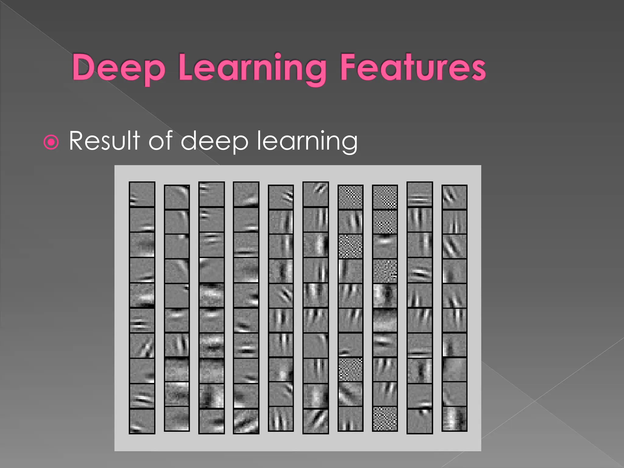
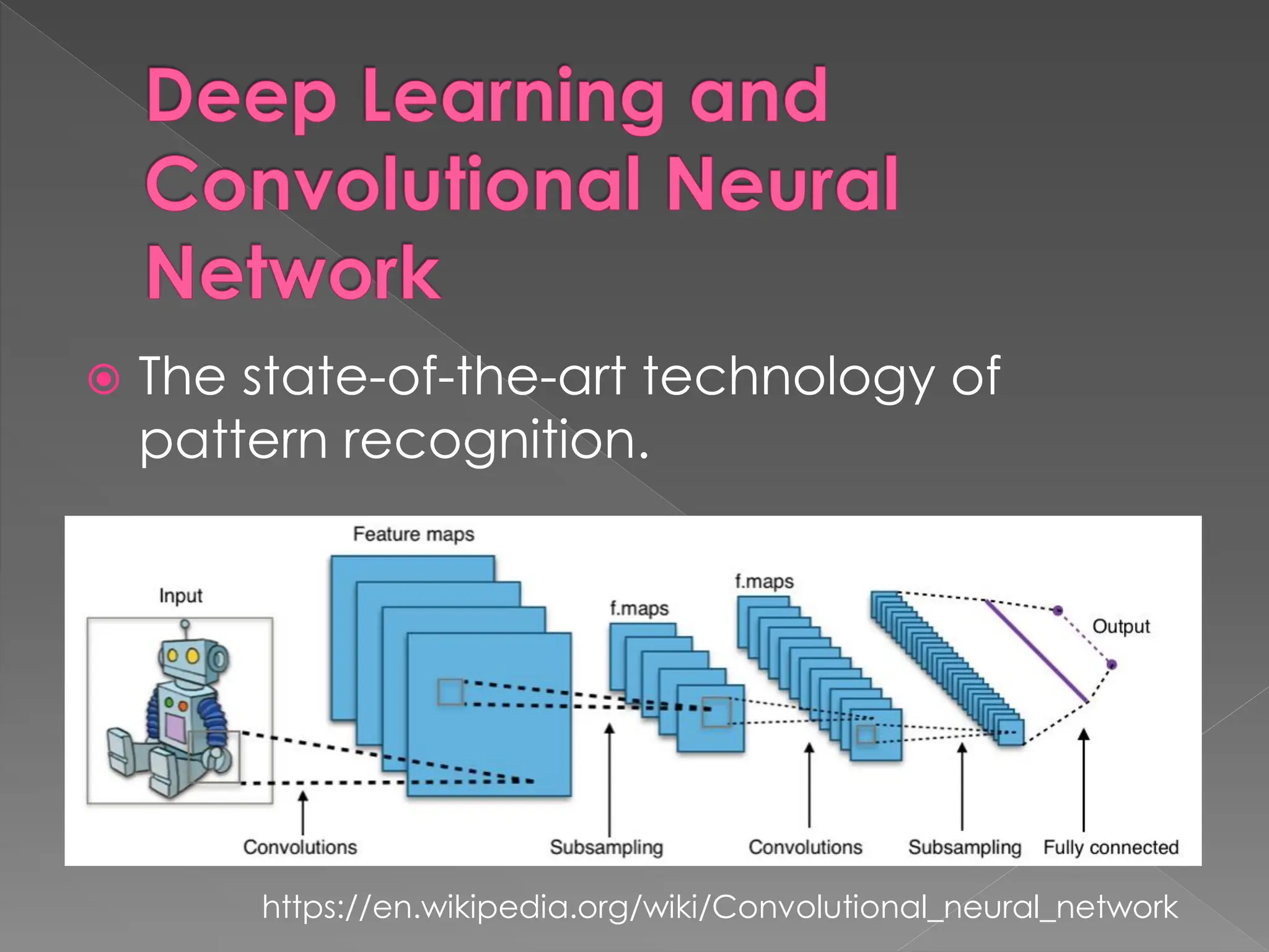
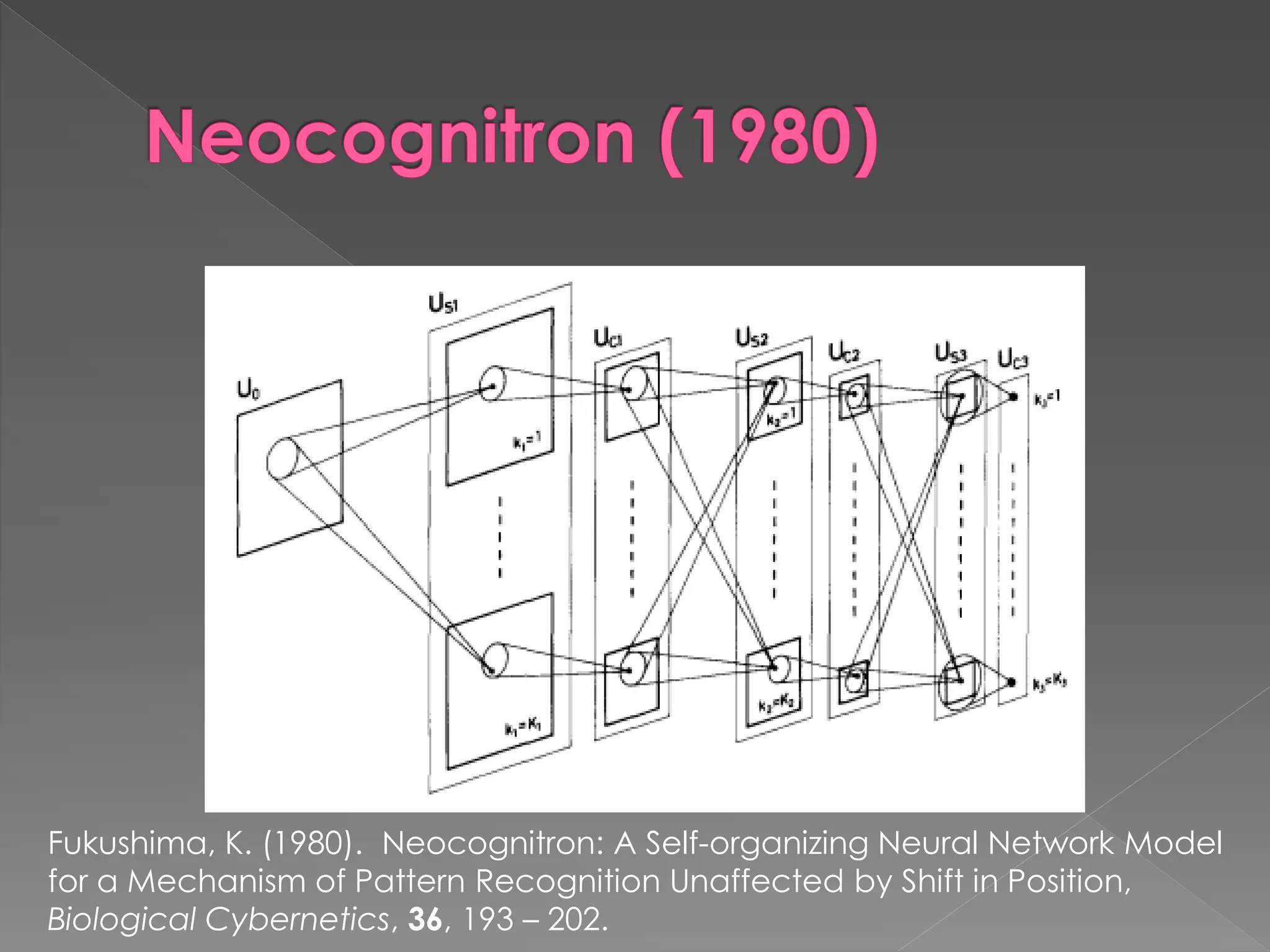
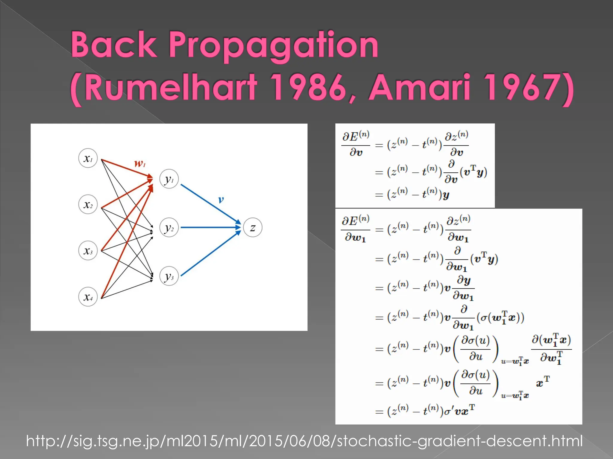
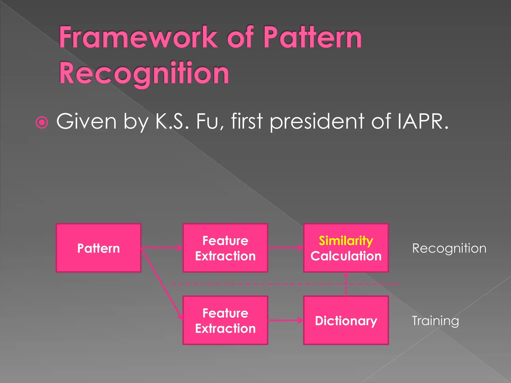
Pattern Recognition Revisited
Another Story of Pattern Recognition
Is Deep Learning the only way?
Ken-ichi Maeda
ICVSS: Sicily, 22 July 2016
Deep Learning and
Convolutional Neural
Network
 The state-of-the-art technology of
pattern recognition.
https://en.wikipedia.org/wiki/Convolutional_neural_network
Neocognitron (1980)
Fukushima, K. (1980). Neocognitron: A Self-organizing Neural Network Model
for a Mechanism of Pattern Recognition Unaffected by Shift in Position,
Biological Cybernetics, 36, 193 – 202.
Back Propagation
(Rumelhart 1986, Amari 1967)
http://sig.tsg.ne.jp/ml2015/ml/2015/06/08/stochastic-gradient-descent.html
Framework of Pattern
Recognition
 Given by K.S. Fu, first president of IAPR.
Feature
Extraction
Similarity
Calculation
Pattern Recognition
Dictionary
Feature
Extraction
Training
Framework of Pattern
Recognition
 Similar to 3-layer Neural Network?
Input Hidden Layer Output
Pattern Feature Extraction Similarity
What is Feature?
 Edge, corner, whiteness/blackness,
direction of vector (correlation of
meshes)
Neocognitron (1980)
Fukushima, K. (1980). Neocognitron: A Self-organizing Neural Network Model
for a Mechanism of Pattern Recognition Unaffected by Shift in Position,
Biological Cybernetics, 36, 193 – 202.
Layered Features
 3-Layer Neural Network
Pattern Feature Extraction Similarity
Layered Features
 4-Layer Neural Network
Pattern
Feature
Extraction 1
Similarity
Feature
Extraction 2
ASPET 70/71 (1970, 1971)
 Analog Spatial Processor Developed by
Electro-Technical Laboratory and
Toshiba
 OCR prototype
http://museum.ipsj.or.jp/en/heritage/ASPET/71.html
Analog Spatial Processor
 Composed by analog IC and resistor
network
Op
Amp
R2
R3
R1
R4
Feature Extraction
 Geometric Feature: Whiteness/blackness
convolution with Gaussian Function (Pool)
𝑓(𝒓𝑖, 𝜎) = න 𝐺 𝒓𝑖 − 𝒓, 𝜎 𝑓(𝒓)d𝒓
𝐺 𝒓, 𝜎 =
1
2π𝜎2 exp −
𝒓 2
2𝜎2
Feature Extraction
 Statistical Feature: Vector directions (m)
calculated using PCA
𝒇, 𝝋𝑚
𝐾𝝋𝑚 = 𝜆𝑚𝝋𝑚
𝐾 = ෍
𝛼
𝑤𝛼 𝒇𝛼, 𝒇𝛼
Similarity
 Multiple Similarity Measure: Angle
between Vector and Subspace
𝑆 𝒇 = cos 2 𝜃
= ෍
𝑚=1
𝑀
𝒇, 𝝋𝑚
2
𝒇 2
Similarity Visualisation
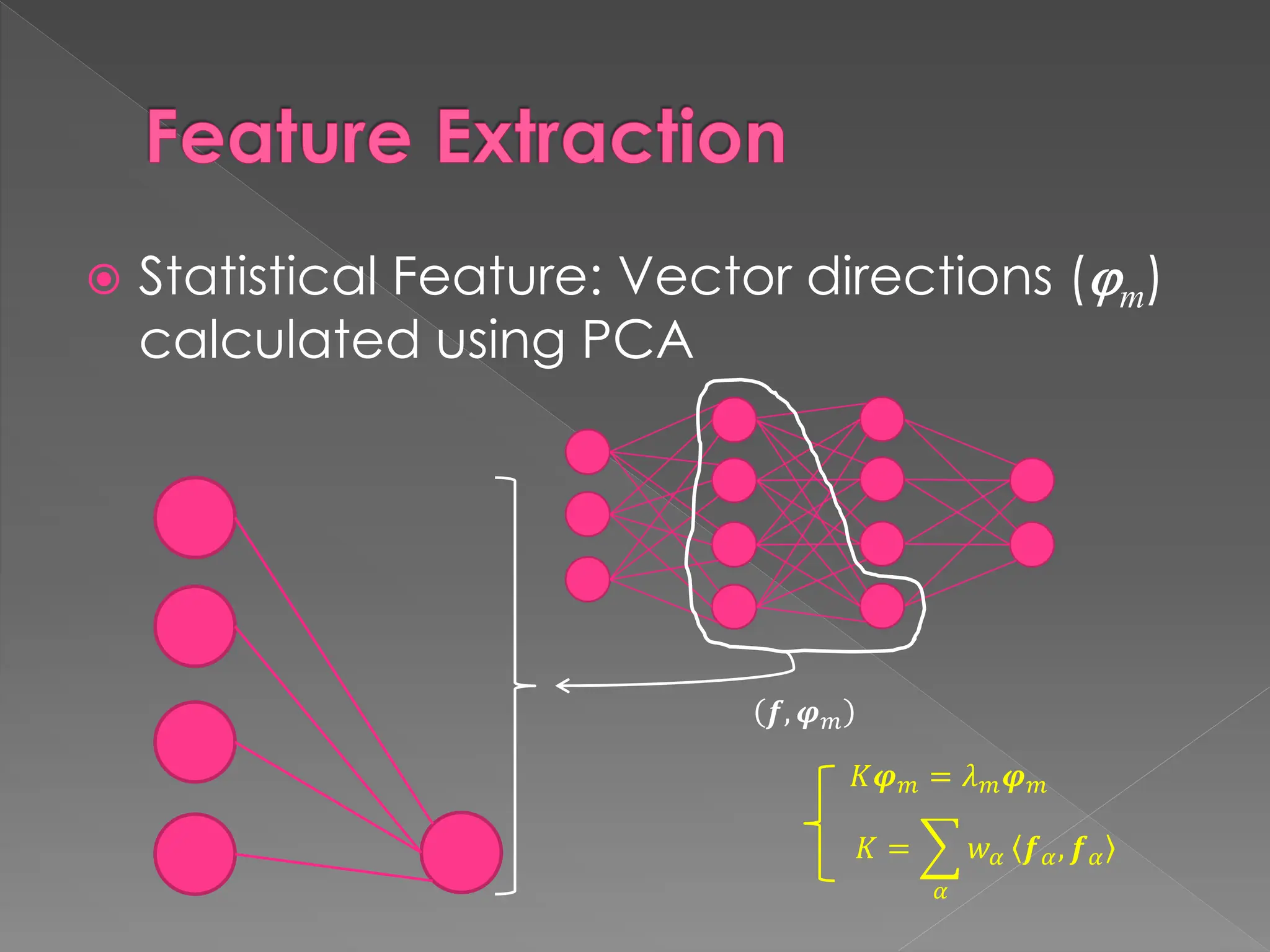
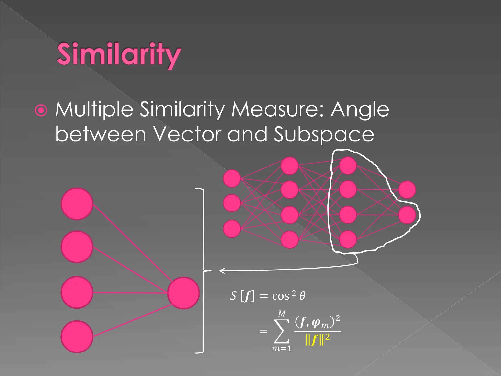
 Angle between a vector and a subspace
(f*: Nearest vector of f in the subspace)
S [f] = cos2 
𝝋1
𝝋2
f

f*
Problems in Features
 Is convolution with Gaussian Function
effective enough to recognize Kanji
(Chinese characters)?
Extended Features
 We need more complex features, e.g.,
edges
› Gaussian-weighted Hermite Polynomials
𝒓 = 𝑥𝒊 + 𝑦𝒋
𝜕𝑚+𝑛
𝜕𝑥𝑚𝜕𝑦𝑛 𝑓 𝒓, 𝜎 = න
𝜕𝑚+𝑛
𝜕𝑥𝑚𝜕𝑦𝑛 𝐺 𝒓 − 𝒓′
, 𝜎 𝑓(𝒓′)d𝒓′
=
𝑚!𝑛!
− 2
𝑚+𝑛 𝑓𝑚𝑛 𝒓, 𝜎
𝑓𝑚𝑛 𝒓, 𝜎 = න
1
𝑚! 𝑛!
𝜎
2
𝑚+𝑛 𝐺 𝒓 − 𝒓′, 𝜎 𝐻𝑚
𝑥 − 𝑥′
𝜎
𝐻𝑛(
𝑦 − 𝑦′
𝜎
)𝑓(𝒓′)d𝒓′
Basic Equation of Figure and
Scale Space
 Proposed by Iijima (1959) before scale
space by Witkin (1983).
𝑓(𝒓𝑖, 𝜎) = න 𝐺 𝒓𝑖 − 𝒓, 𝜎 𝑓(𝒓)d𝒓
𝛁2 −
𝜕
𝜕𝜏
𝑓 𝒓, 𝜎 = 0
𝜏 =
𝜎2
2
Gaussian-weighted Hermite
Polynomials (Maeda 1982)
 Like Gabor Functions
Similar Feature (Gabor)
 Equal interval 0 crossing
Similar Feature (Rubner 1990)
 Made using Oja’s equation.
 Look like Gaussian-weighted Hermite
Polynomials
Similar Feature (Linsker 1988)
 Layered Linsker Network
Similar Feature (MacKay
1990)
 Polar Representation
Deep Learning Features
 Result of deep learning
Hebbian Learning
 A basic concept of correlation learning
presented by Hebb (1949)
› 𝑥𝑖 input, 𝑦 output, 𝑤𝑖 connection,
𝜂 learning weight
∆𝑤𝑖 = 𝜂𝑥𝑖𝑦
𝑦 = ෍
𝑗
𝑤𝑗 𝑥𝑗
Modified Learning
 Oja (1982) showed that a neuron model
could generate a subspace {𝝋m}.
› 𝜉𝑖 input, 𝜇𝑖 connection, 𝜂 output
› Modified learning equation assuming 𝛾
(positive learning parameter) is small.
𝜇𝑖 𝑡 + 1 = 𝜇𝑖 𝑡 + 𝛾𝜂 𝑡 𝜉𝑖 𝑡 − 𝜂 𝑡 𝜇𝑖 𝑡 + 𝑂 𝛾2
𝝋𝑚 = T(𝜇1, 𝜇2, ⋯ , 𝜇𝑖, ⋯ , 𝜇𝐼)
𝜇𝑖 𝑡 + 1 =
𝜇𝑖 𝑡 + 𝛾𝜂 𝑡 𝜉𝑖 𝑡
σ𝑗=1
𝐼
𝜇𝑖 𝑡 + 𝛾𝜂 𝑡 𝜉𝑖 𝑡 2 1/2 (original modification)
Modified Learning
 von der Malsburg (1985) showed a set of
learning neurons form a columnar
structure also with discarding higher
order.
› 𝑊𝑖𝑗 connection
ሶ
𝑊𝑖𝑗 = 𝑊𝑖𝑗 𝑊 𝑖𝑗
2
− 𝑊𝑖𝑗 ෍
𝑖′
𝑊𝑖′𝑗 𝑊 𝑖′𝑗
2
+ ෍
𝑗′
𝑊𝑖𝑗′ 𝑊 𝑖𝑗′
2
𝑊2
= 𝑊 A static solution
What is Learning?
 Learning is used to find geometric
features.
 Learning is the training phase for
recognition.
› To find correlation features.
Back Propagation
(Rumelhart 1986, Amari 1967)
http://sig.tsg.ne.jp/ml2015/ml/2015/06/08/stochastic-gradient-descent.html
Learning Subspace Method
(1979)
Maeda, K. (1990). Dimension Selection by Learning for Class Discrimination
and Information Representation. AIAI Technical Reports, AIAI-TR-75.
𝐴′
= 𝐸 ± 𝛿
𝒇, 𝒇
𝒇 2 𝐴
A : projection
E : unit matrix
To learn an input 𝒇 ,
Averaged Learning Subspace
Method (Kuusela 1982, Maeda
1980)
Maeda, K. (1990). Dimension Selection by Learning for Class Discrimination
and Information Representation. AIAI Technical Reports, AIAI-TR-75.
To learn an input 𝒇 ,
𝐾′ = 1 ∓ 𝛿 𝐾 ± 𝛿
𝒇, 𝒇
𝒇 2 𝐾 : PCA correlation matrix
Conclusion
 Deep Learning is the state-of-the-art
technique in pattern recognition and
machine learning, but similar concepts
and results existed before.
 It is quite a powerful method, but is not
the only solution.
 We sometimes should return to the
principle, so that we can continue
making progress.
Guidance on the future
 Learn from the past, but never stick to it
only.
 Back to the principle, back to what you
see.
 Everything is useful if you can correctly
see.
The future is yours!
References of Historical Works
 Amari, S. (1967). Theory of Adaptive Pattern Classifiers, IEEE Transactions EC-1, 299–307.
 Fukushima, K. (1980). Neocognitron: A Self-organizing Neural Network Model for a Mechanism of Pattern Recognition
Unaffected by Shift in Position, Biological Cybernetics, 36, 193 – 202.
 Hebb, D. O. (1949). The Organization of Behavior, Wiley.
 Hubel, D. H. and Wiesel, T. N. (1962). Receptive Fields, Binocular Interaction, and Fundamental Architecture in the Cat's Visual
Cortex, J. Physiol., 160, 106-154.
 Iijima, T. (1959). Basic Theory of Pattern Observation, Technical Group on Automata and Automatic Control, IECE, 1-37. In
Japanese.
 Iijima, T. (1963). Basic Theory of Feature Extraction from Visual Patterns, J. IECE, 46 (11), 1714. In Japanese.
 Iijima, T., et al. (1972). A Theoretical Study of Pattern Identification by Matching Method in Proc. of First USA-Japan Computer
Conf., 42–48.
 Iijima, T., et al. (1973). A Theory of Character Recognition by Pattern Matching Method, Proc. of First Int. Joint Conf. on Pattern
Recognition, 50-56.
 Irie, B. and Miyake, S. (1988). Capabilities of Three-Layered Perceptrons, Proc. of ICNN, Vol. 1, 641 – 648.
 Kohohen, T. et al. (1979). Spectral Classification of Phoneme by Learning Subspace, Proc. of Int. Conf. on Acoustics, Speech,
and Signal Processing, 807 – 809.
 Kuusela, M and Oja, E. (1982). Averaged Learning Subspace Method for Spectral Pattern Recognition, Proc. Of the 6th Int.
Cong. on Pattern Recognition (ICPR ‘82), 134 – 137.
 Linsker, R. (1988). Self-Organization in a Perceptual Network, Computer, 21 (3), 105-117.
 MacKay, D. J. C., et al. (1990). Analysis of Linsker's Simulations of Hebbian Rules, Neural Computation, 2 (2), 173-187.
 Maeda, K. (1980). Pattern Recognition Apparatus, Japanese Patent Public Disclosure, 137483/81, 1980
 Maeda, K., et al. (1982). Hand-printed Kanji Recognition by Pattern Matching Method, Proc. of the 6th Int. Conf. on Pattern
Recognition (ICPR '82), 789–792.
 Maeda, K. (1990). Dimension Selection by Learning for Class Discrimination and Information Representation. AIAI Technical
Reports, AIAI-TR-75.
 von der Malsburg, C. (1985). Nervous Structures with Dynamical Links, Ber. Bunsenges. Phys. Chem., 89, 703-710.
 Oja, E. (1982). A Simplified Neuron Model as a Principal Component Analyzer, J. Math. Biology, 15 (3), 267-273.
 Rubner, J., et al. (1990). A Self-Organizing Network for Complete Feature Extraction, Proc. of Int. Conf. on Parallel Processing in
Neural Systems and Computers, 365-368.
 Rumelhart, David E.; Hinton, Geoffrey E., Williams, Ronald J. (1986). Learning representations by back-propagating errors,
Nature 323 (6088): 533–536.
 Widrow, B., et al. (1960). Adaptive Switching Circuits, IRE WESCON Convention Record 4: 96-104.
 Witkin, A. P. (1983). Scale-space filtering, Proc. 8th Int. Joint Conf. Art. Intell.,1019–1022.

Pattern Recognition Revisited, ICVSS 2016 presentaion

  • 1.
    Pattern Recognition Revisited AnotherStory of Pattern Recognition Is Deep Learning the only way? Ken-ichi Maeda ICVSS: Sicily, 22 July 2016
  • 2.
    Deep Learning and ConvolutionalNeural Network  The state-of-the-art technology of pattern recognition. https://en.wikipedia.org/wiki/Convolutional_neural_network
  • 3.
    Neocognitron (1980) Fukushima, K.(1980). Neocognitron: A Self-organizing Neural Network Model for a Mechanism of Pattern Recognition Unaffected by Shift in Position, Biological Cybernetics, 36, 193 – 202.
  • 4.
    Back Propagation (Rumelhart 1986,Amari 1967) http://sig.tsg.ne.jp/ml2015/ml/2015/06/08/stochastic-gradient-descent.html
  • 5.
    Framework of Pattern Recognition Given by K.S. Fu, first president of IAPR. Feature Extraction Similarity Calculation Pattern Recognition Dictionary Feature Extraction Training
  • 6.
    Framework of Pattern Recognition Similar to 3-layer Neural Network? Input Hidden Layer Output Pattern Feature Extraction Similarity
  • 7.
    What is Feature? Edge, corner, whiteness/blackness, direction of vector (correlation of meshes)
  • 8.
    Neocognitron (1980) Fukushima, K.(1980). Neocognitron: A Self-organizing Neural Network Model for a Mechanism of Pattern Recognition Unaffected by Shift in Position, Biological Cybernetics, 36, 193 – 202.
  • 9.
    Layered Features  3-LayerNeural Network Pattern Feature Extraction Similarity
  • 10.
    Layered Features  4-LayerNeural Network Pattern Feature Extraction 1 Similarity Feature Extraction 2
  • 11.
    ASPET 70/71 (1970,1971)  Analog Spatial Processor Developed by Electro-Technical Laboratory and Toshiba  OCR prototype http://museum.ipsj.or.jp/en/heritage/ASPET/71.html
  • 12.
    Analog Spatial Processor Composed by analog IC and resistor network Op Amp R2 R3 R1 R4
  • 13.
    Feature Extraction  GeometricFeature: Whiteness/blackness convolution with Gaussian Function (Pool) 𝑓(𝒓𝑖, 𝜎) = න 𝐺 𝒓𝑖 − 𝒓, 𝜎 𝑓(𝒓)d𝒓 𝐺 𝒓, 𝜎 = 1 2π𝜎2 exp − 𝒓 2 2𝜎2
  • 14.
    Feature Extraction  StatisticalFeature: Vector directions (m) calculated using PCA 𝒇, 𝝋𝑚 𝐾𝝋𝑚 = 𝜆𝑚𝝋𝑚 𝐾 = ෍ 𝛼 𝑤𝛼 𝒇𝛼, 𝒇𝛼
  • 15.
    Similarity  Multiple SimilarityMeasure: Angle between Vector and Subspace 𝑆 𝒇 = cos 2 𝜃 = ෍ 𝑚=1 𝑀 𝒇, 𝝋𝑚 2 𝒇 2
  • 16.
    Similarity Visualisation  Anglebetween a vector and a subspace (f*: Nearest vector of f in the subspace) S [f] = cos2  𝝋1 𝝋2 f  f*
  • 17.
    Problems in Features Is convolution with Gaussian Function effective enough to recognize Kanji (Chinese characters)?
  • 18.
    Extended Features  Weneed more complex features, e.g., edges › Gaussian-weighted Hermite Polynomials 𝒓 = 𝑥𝒊 + 𝑦𝒋 𝜕𝑚+𝑛 𝜕𝑥𝑚𝜕𝑦𝑛 𝑓 𝒓, 𝜎 = න 𝜕𝑚+𝑛 𝜕𝑥𝑚𝜕𝑦𝑛 𝐺 𝒓 − 𝒓′ , 𝜎 𝑓(𝒓′)d𝒓′ = 𝑚!𝑛! − 2 𝑚+𝑛 𝑓𝑚𝑛 𝒓, 𝜎 𝑓𝑚𝑛 𝒓, 𝜎 = න 1 𝑚! 𝑛! 𝜎 2 𝑚+𝑛 𝐺 𝒓 − 𝒓′, 𝜎 𝐻𝑚 𝑥 − 𝑥′ 𝜎 𝐻𝑛( 𝑦 − 𝑦′ 𝜎 )𝑓(𝒓′)d𝒓′
  • 19.
    Basic Equation ofFigure and Scale Space  Proposed by Iijima (1959) before scale space by Witkin (1983). 𝑓(𝒓𝑖, 𝜎) = න 𝐺 𝒓𝑖 − 𝒓, 𝜎 𝑓(𝒓)d𝒓 𝛁2 − 𝜕 𝜕𝜏 𝑓 𝒓, 𝜎 = 0 𝜏 = 𝜎2 2
  • 20.
    Gaussian-weighted Hermite Polynomials (Maeda1982)  Like Gabor Functions
  • 21.
    Similar Feature (Gabor) Equal interval 0 crossing
  • 22.
    Similar Feature (Rubner1990)  Made using Oja’s equation.  Look like Gaussian-weighted Hermite Polynomials
  • 23.
    Similar Feature (Linsker1988)  Layered Linsker Network
  • 24.
  • 25.
    Deep Learning Features Result of deep learning
  • 26.
    Hebbian Learning  Abasic concept of correlation learning presented by Hebb (1949) › 𝑥𝑖 input, 𝑦 output, 𝑤𝑖 connection, 𝜂 learning weight ∆𝑤𝑖 = 𝜂𝑥𝑖𝑦 𝑦 = ෍ 𝑗 𝑤𝑗 𝑥𝑗
  • 27.
    Modified Learning  Oja(1982) showed that a neuron model could generate a subspace {𝝋m}. › 𝜉𝑖 input, 𝜇𝑖 connection, 𝜂 output › Modified learning equation assuming 𝛾 (positive learning parameter) is small. 𝜇𝑖 𝑡 + 1 = 𝜇𝑖 𝑡 + 𝛾𝜂 𝑡 𝜉𝑖 𝑡 − 𝜂 𝑡 𝜇𝑖 𝑡 + 𝑂 𝛾2 𝝋𝑚 = T(𝜇1, 𝜇2, ⋯ , 𝜇𝑖, ⋯ , 𝜇𝐼) 𝜇𝑖 𝑡 + 1 = 𝜇𝑖 𝑡 + 𝛾𝜂 𝑡 𝜉𝑖 𝑡 σ𝑗=1 𝐼 𝜇𝑖 𝑡 + 𝛾𝜂 𝑡 𝜉𝑖 𝑡 2 1/2 (original modification)
  • 28.
    Modified Learning  vonder Malsburg (1985) showed a set of learning neurons form a columnar structure also with discarding higher order. › 𝑊𝑖𝑗 connection ሶ 𝑊𝑖𝑗 = 𝑊𝑖𝑗 𝑊 𝑖𝑗 2 − 𝑊𝑖𝑗 ෍ 𝑖′ 𝑊𝑖′𝑗 𝑊 𝑖′𝑗 2 + ෍ 𝑗′ 𝑊𝑖𝑗′ 𝑊 𝑖𝑗′ 2 𝑊2 = 𝑊 A static solution
  • 29.
    What is Learning? Learning is used to find geometric features.  Learning is the training phase for recognition. › To find correlation features.
  • 30.
    Back Propagation (Rumelhart 1986,Amari 1967) http://sig.tsg.ne.jp/ml2015/ml/2015/06/08/stochastic-gradient-descent.html
  • 31.
    Learning Subspace Method (1979) Maeda,K. (1990). Dimension Selection by Learning for Class Discrimination and Information Representation. AIAI Technical Reports, AIAI-TR-75. 𝐴′ = 𝐸 ± 𝛿 𝒇, 𝒇 𝒇 2 𝐴 A : projection E : unit matrix To learn an input 𝒇 ,
  • 32.
    Averaged Learning Subspace Method(Kuusela 1982, Maeda 1980) Maeda, K. (1990). Dimension Selection by Learning for Class Discrimination and Information Representation. AIAI Technical Reports, AIAI-TR-75. To learn an input 𝒇 , 𝐾′ = 1 ∓ 𝛿 𝐾 ± 𝛿 𝒇, 𝒇 𝒇 2 𝐾 : PCA correlation matrix
  • 33.
    Conclusion  Deep Learningis the state-of-the-art technique in pattern recognition and machine learning, but similar concepts and results existed before.  It is quite a powerful method, but is not the only solution.  We sometimes should return to the principle, so that we can continue making progress.
  • 34.
    Guidance on thefuture  Learn from the past, but never stick to it only.  Back to the principle, back to what you see.  Everything is useful if you can correctly see. The future is yours!
  • 35.
    References of HistoricalWorks  Amari, S. (1967). Theory of Adaptive Pattern Classifiers, IEEE Transactions EC-1, 299–307.  Fukushima, K. (1980). Neocognitron: A Self-organizing Neural Network Model for a Mechanism of Pattern Recognition Unaffected by Shift in Position, Biological Cybernetics, 36, 193 – 202.  Hebb, D. O. (1949). The Organization of Behavior, Wiley.  Hubel, D. H. and Wiesel, T. N. (1962). Receptive Fields, Binocular Interaction, and Fundamental Architecture in the Cat's Visual Cortex, J. Physiol., 160, 106-154.  Iijima, T. (1959). Basic Theory of Pattern Observation, Technical Group on Automata and Automatic Control, IECE, 1-37. In Japanese.  Iijima, T. (1963). Basic Theory of Feature Extraction from Visual Patterns, J. IECE, 46 (11), 1714. In Japanese.  Iijima, T., et al. (1972). A Theoretical Study of Pattern Identification by Matching Method in Proc. of First USA-Japan Computer Conf., 42–48.  Iijima, T., et al. (1973). A Theory of Character Recognition by Pattern Matching Method, Proc. of First Int. Joint Conf. on Pattern Recognition, 50-56.  Irie, B. and Miyake, S. (1988). Capabilities of Three-Layered Perceptrons, Proc. of ICNN, Vol. 1, 641 – 648.  Kohohen, T. et al. (1979). Spectral Classification of Phoneme by Learning Subspace, Proc. of Int. Conf. on Acoustics, Speech, and Signal Processing, 807 – 809.  Kuusela, M and Oja, E. (1982). Averaged Learning Subspace Method for Spectral Pattern Recognition, Proc. Of the 6th Int. Cong. on Pattern Recognition (ICPR ‘82), 134 – 137.  Linsker, R. (1988). Self-Organization in a Perceptual Network, Computer, 21 (3), 105-117.  MacKay, D. J. C., et al. (1990). Analysis of Linsker's Simulations of Hebbian Rules, Neural Computation, 2 (2), 173-187.  Maeda, K. (1980). Pattern Recognition Apparatus, Japanese Patent Public Disclosure, 137483/81, 1980  Maeda, K., et al. (1982). Hand-printed Kanji Recognition by Pattern Matching Method, Proc. of the 6th Int. Conf. on Pattern Recognition (ICPR '82), 789–792.  Maeda, K. (1990). Dimension Selection by Learning for Class Discrimination and Information Representation. AIAI Technical Reports, AIAI-TR-75.  von der Malsburg, C. (1985). Nervous Structures with Dynamical Links, Ber. Bunsenges. Phys. Chem., 89, 703-710.  Oja, E. (1982). A Simplified Neuron Model as a Principal Component Analyzer, J. Math. Biology, 15 (3), 267-273.  Rubner, J., et al. (1990). A Self-Organizing Network for Complete Feature Extraction, Proc. of Int. Conf. on Parallel Processing in Neural Systems and Computers, 365-368.  Rumelhart, David E.; Hinton, Geoffrey E., Williams, Ronald J. (1986). Learning representations by back-propagating errors, Nature 323 (6088): 533–536.  Widrow, B., et al. (1960). Adaptive Switching Circuits, IRE WESCON Convention Record 4: 96-104.  Witkin, A. P. (1983). Scale-space filtering, Proc. 8th Int. Joint Conf. Art. Intell.,1019–1022.