SlideShare a Scribd company logo
1 of 162
Optimal Debt Mix and Priority Structure:
The Role of Bargaining Power∗
DirkHackbarth ChristopherA.Hennessy HayneE.Leland
April 25, 2002
ABSTRACT
This paper examines the optimal priority structure and mix of
bank and bond market debt
within a continuous-time asset pricing framework. Closed-form
expressions are derived for the
values of renegotiable bank debt, non-renegotiable bond market
debt, equity, and levered firm
values. We show that the optimal debt structure hinges upon the
ex post division of bargaining
power between the firm and bank. The optimal debt structure
for firms that are weak vis-à-vis
the bank entails financing exclusively with bank debt. Strong
firms find it optimal to issue a
mix of bank and bond market debt, with the bank senior in the
priority structure. The model
explains: (i) why it is optimal for small firms to avoid public
debt markets, (ii) why large firms
employ mixed debt financing (iii) why banks are senior in the
priority structure, and (iv) why
firms shift from bank debt into a mixture of bond market and
bank debt over their life-cycle.
These predictions are generated within a tax shield-bankruptcy
cost tradeoff model in which
the only unique feature of banks is their ability to renegotiate.
JEL Codes: G13, G32, G33.
Keywords: Banking, Capital Structure, Priority Structure, and
Contingent Claims Pricing.
∗ PRELIMINARY AND INCOMPLETE. The authors are from
the Haas School of Business, U.C. Berkeley.
I. Introduction
In the years following the publication of the Modigliani and
Miller (MM, 1958) irrelevancy result,
debt tax shields and the costs of default or bankruptcy have
been cited as important determinants
of a firm’s optimal capital structure. A common shortcoming of
this literature is that it typically
ignores lender heterogeneity. However, debt contracts are
shaped in critical ways by the type of
lender and the division of bargaining power between borrower
and lender in the event ofnonpayment
of initially-promised amounts (a “renegotiation”). For instance,
bank debt is typically soft in the
sense that its terms can be renegotiated without necessarily
incurring formal default or bankruptcy,
while bond market debt is typically hard, in that renegotiation
with dispersed creditors is costly or
impossible and may well lead to formaldefault and/or
bankruptcy.1 Costs, both directand indirect,
are generally incurred in bankruptcy.2 In addition, the outcome
of the debt renegotiation process
itself is influenced by the division of bargaining power between
lenders and the firm whenever the
firm chooses not to make the promised debt service.
Renegotiation between the firm and lenders
is also affected by the priority structure of debt, which affects
the threat points of heterogeneous
lenders.
This paper examines the effect of debt heterogeneity and
priority structure on the value of the
corporate tax shield, bankruptcy costs,and renegotiation costs
within the context of a continuous-
time asset pricing framework. We solve for the optimal priority
structure and mix of renegotiable
bank debt and non-renegotiable bond market debt. It is shown
that the optimal debt struc-
ture depends critically upon the ex post division of bargaining
power between the firm and bank.
Throughout the paper, the term ex ante refers to times prior to
the issuance of debt contracts,
while ex post refers to times when the firm’s debt structure is in
place. By optimal financial
structure, we mean the debt mix and priority structure that
maximizes the ex ante value of all
marketable claims on the firm.
We consider two polar cases regarding the distribution of
bargaining power: when the firm is
strong, in which case the firm can offer reduced debt service
that just avoids the bank’s demand
1Bondholders acting atomistically may hold out and preclude
desirable debt restructuring; cf. Gertner and Scharf-
stein (1991), Brown, James, and Mooradian (1993), Kahan and
Tuckman (1993), and Morris and Shin (2001).
Further, informational asymmetries can make Chapter 11 more
attractive for individual bondholders than private
debt reorganizations; cf. Giammarino (1991).
2See Warner (1977), Altman (1984), Summers and Cutler
(1988), Weiss (1990), Franks and Torous (1989, 1994),
and Andrade and Kaplan (1998).
1
for liquidation; or when the firm is weak, in which case the
bank can demand payments which just
avoid the firm’s refusing to pay and voluntarily declaring
bankruptcy. In particular, we address
four related questions: (i) If the choice between bond market
and bank debt is mutually exclusive,
which should be chosen? (ii) If the firm may issue both bond
market and bank debt, what is the
optimal mix of the two? (iii) What is the optimal priority
structure when multiple debt classes
are issued? (iv) How does the ex post division of bargaining
power between the firm and lending
bank(s) affect the answer to each of these questions?3
These questions are addressed using a unified continuous-time
asset pricing framework that
bridges the gap between the Leland (1994) model, which treats
non-renegotiable debt, and the
model of Mella-Barral and Perraudin (MBP, 1997) which
features renegotiable debt. Analytical
solutions are derived for bank debt, bond market debt, equity,
and levered firm values as func-
tions of the endogenously determined variables (promised
coupon payments and priority structure)
and exogenous parameters (ex post bargaining power,
underlying volatility, corporate tax rates,
negotiation costs, and bankruptcy costs).
The model generates several predictions that are supported by
empirical observation. First,
weak firms, those ceding all bargaining power to banks in the
event of renegotiation, find it optimal
to finance exclusively with bank debt. That is, for weak firms,
bank debt dominates any mix
of bond market and bank debt, regardless of the priority
structure under the mixed debt policy.
This result holds in the absence of any notion of monitoring or
certification by banks, transaction
costs, economies of scale, and other common rationales for why
small firms fail to tap public debt
markets. Second, for strong firms, those with full bargaining
power in renegotiations with banks,
the optimal financial structure entails a mixture of bank and
bond market debt. In particular,
the analysis indicates that there is a complementarity effect
between bank debt and bond market
debt for strong firms. Thus, the model provides a rationale for
the coexistence of bank debt
(indirect or intermediated finance) and bond market debt (direct
finance). Third, for reasonable
parameter values, it is optimal for strong firms that optimally
choose mixed debt to place bank debt
senior. Intuitively, placing the bank senior in the priority
structure raises the bank’s reservation
value, which thereby commits equity to higher debt service in
renegotiations. The increase in debt
3Ex post bargaining power in our model is not ex ante
contractible and therefore exogenous. Note that when
renegotiations commence, both sides will want maximal
bargaining power. Thus, a non-contracted “agreement” to
be weak is incentive incompatible ex post.
2
service raises the value of both the tax shield and bankruptcy
costs. We find that the former effect
dominates for reasonable parameter values.
To the extent that one views young firms as having a weak ex
post bargaining position vis-à-vis
banks, and gaining bargaining strength as they mature, the
model generates a life-cycle hypothesis
for debt structure. Young firms begin by relying exclusively on
bank debt. As they grow and gain
bargaining power, they shift away from bank debt, placing more
reliance on bond market debt.
This prediction is consistent with observed financing patterns,
and is not dependent on the notion
of bank certification. In fact, the model predicts that even if a
weak firm could tap public debt
markets with fair pricing, it would be sub-optimal to do so.
Finally, when the choice between bank and bond market debt is
mutually exclusive, we find
that the optimal debt structure of strong firms depends on their
level of bankruptcy costs and tax
shield values. Interestingly, strong firms are ceteris paribus
more likely to choose bond market
over bank debt when bankruptcy costs are high. Taken together,
these results suggest the more
general conclusion that bank debt is relatively more desirable to
firms ex ante when banks have a
stronger bargaining position in renegotiations. For instance,
pure bank debt financing is strictly
preferred to any mixture of bond market and bank debt when
banks are strong and firms are weak.
When firms are strong and optimally seek a mixture of bank and
bond market financing, bank debt
seniority–which improves the threat point of the bank–is
optimal ex ante for the firm. When
firms are strong and financing is mutually exclusive, bank debt
will be preferred when bankruptcy
costs are low, since low bankruptcy costs raise the threat point
of the bank in renegotiations.
The remainder of the paper is organized as follows. Section II
contains a review of the related
empirical and theoretical literature. Section III presents the
model. The contingent claims on the
levered firm are valued in Section IV. Section V analyzes the
case of mutually exclusive financing
choices and Section VI contains the analysis of the mixed debt
firm. Section VII concludes.
II. Literature Review
A number of papers have incorporated strategic interactions
between debt and equity as well as
debt renegotiation in the context of contingent claims valuation
models. Anderson and Sundaresan
(1996) examine strategic debt service in a Cox-Ross-Rubinstein
binomial-tree setting, while MBP
3
(1997) studies a continuous-time model of debt renegotiation.
More recently, Fan and Sundaresan
(2000) characterize two Nash bargaining formulations in which
equity and debt bargain over the
value of the assets of the firm (debt-equity swap) or over the
value of the firm (strategic debt
service).
Our model may be viewed as bridging the gap between Leland
(1994) and MBP (1997). Leland
(1994) represents a unified theory of optimal leverage when the
firm may only issue non-renegotiable
debt. Optimal leverage is chosen to maximize the value of tax
shield benefits less bankruptcy costs.
MBP (1997) analyze a firm that may only issue renegotiable
debt, with bargaining power treated as
a choice variable. In their continuous-time model, they show
that strategic debt service eliminates
direct bankruptcy costs as well as inefficient liquidation. This
result restores the Modigliani-Miller
irrelevance result of financial policy, since there are no tax
benefits in their basic model. In the
presence of tax shields, they argue that distributing all
bargaining power to the bank is optimal.
Since the Leland (1994) and MBP (1997) papers analyze
situations in which the firm issues
only a single class of debt, the question of the optimal mix
between bank and bond market debt
is beyond the scope of their papers. Similarly, the question of
the optimal priority structure is
left unaddressed.4 The present paper stresses the notion that in
many settings the distribution of
ex post bargaining power must be taken as a given by the firm,
and cannot be treated as a choice
variable. Therefore, even in settings where a particular
distribution of bargaining power may be
said to dominate in the sense of resulting in higher firm
valuations, the firm may be unable to
commit to such a division of bargaining power, and must
optimize subject to this constraint.
It has been well documented empirically that banks are
generally senior in the priority structure.
For example, Carey (1995) finds that in the 18,000 loans made
between 1986 and 1993 and recorded
in theDealscan database, over 99percentof all bank
loanscontaina senior priority clause, regardless
of whether or not the borrower has bond market debt
outstanding. Mann (1997) and Schwartz
(1997) find that in addition to taking senior positions, banks
also collateralize as much of their debt
as possible and incorporate protective covenants limiting the
ability of the firm to issue additional
debt.
4Hackbarth and Leland (2001) analyze the role of priority
structure of a firm issuing multiple classes of non-
renegotiable bond market debt.
4
One of the contributions of this paper to the banking literature
is that it suggests an alternative
theory regarding the optimal debt mix and priority structure that
rests upon a standard tax shield-
bankruptcy cost trade-off story. The model does not invoke any
notion of monitoring by the bank,
costly state verification, or asset substitution problems. Yet, it
generates many of the stylized facts
that the banking literature has attempted to explain. This
banking literature is discussed below.
Much of the theoretical banking literature attempts to explain
why banks are senior. Diamond
(1993a, 1993b) develops a model of both adverse selection and
moral hazard, in which he obtains an
optimal debt structure resulting from a trade-off between
informational sensitivity and preservation
of control rent. In his model, because of the non-assignable
control rent, short-term lenders have
excessive incentives to liquidate the firm at the intermediate
date, which imposes a distortion on
long-term lenders. Seniority permits short-term creditors to
dilute the other claims and thereby
moderate their incentives to liquidate the firm early. By
invoking the assumption that renegotiation
of bond market debt is very difficult, he finds that making
short-term (bank) debt senior relative
to long-term (bond market) debt improves the bank’s incentive
to monitor.
Rajan (1992) arrives at the opposite conclusion regarding
priority structure. The main benefit
of bank debt in his model is flexibility in times of distress.
However, banks develop informational
monopolies and can distort investment incentives by demanding
a share of the rents from profitable
projects as a condition for rolling over short-term loans. To
weaken the bargaining power of
informed lenders, the firm grants uninformed lenders higher
priority. Welch (1997) analyzes the
role of influence costs on the optimal priority structure of debt.
Placing bank debt senior is optimal
in his model since influence costs are lower when the strongest
creditor, ex post, is given more power
ex ante.
Repullo and Suarez (1998) abstract from Rajan’s informational
monopoly problem and conclude
that the optimal priority rule entails placing informed lenders
senior. Dewatripont and Tirole
(1994) demonstrate that in order to prevent borrower moral
hazard, it is best for control rights in
bad states to be given to lenders rather than to equity holders
since lenders have a more credible
threat to liquidate the firm. Since equity in their model is
indistinguishable from junior debt, one
can draw many conclusions about the optimal debt and priority
structure from their model. Rajan
and Winton (1995) and Chemmanur and Fulghieri (1994)
propose models of banks as delegated
monitors, but neither analyzes the optimal debt mix or priority
structure.
5
In a first effort to reconcile these two conflicting theories, Park
(2000) develops a theory of
optimal debt structure by explicitly modeling a costly
monitoring technology in a model with asset
substitution. Because thefirm’s contracting costsare reduced
when lendershave stronger incentives
to monitor, firms structure debt securities to maximize the
lenders’ incentives to monitor. This
is achieved only if the delegated monitor can recover all of his
monitoring costs from the lending
relationship, which is feasible only if there are no lenders above
him in the priority structure.
Winton (1995) analyzes the priority structure problem building
on Townsend’s (1979) costly
state verification model. As in the original work, lenders are
assumed to be able to commit
themselves to verification when reported income is low, so that
inspections occur even when banks
know that the firm has truthfully reported low cash flow
truthfully. Winton’s model implies
that junior lenders verify more often than senior lenders, which
is consistent with Fama’s (1990)
intuition.
Diamond’s (1993a, 1993b) theory does not provide a role for
multiple lenders holding different
debt securities of the firm. Extending the model of Hart and
Moore (1998), Berglöf and von
Thadden (1994) develop a rationale for multiple creditors and
seniority structure by illustrating
the role of bargaining power in a renegotiation game of
symmetric information. The main insight is
that the optimal debt contract drives a wedge between short-
term and long-term lenders. Bolton
and Scharfstein (1996) put forth a related model of the optimal
number of creditors. In their
paper, multiple lenders provides a commitment mechanism for
the borrower due to the difficulty of
renegotiating with multiple lenders of the same class.
Our model also generates a life-cycle hypothesis regarding
optimal debt financing policy, which
rests upon a rather different line of causation than that invoked
in the existing banking literature.
Diamond (1991) considers a setting in which banks ignore rents
accruing to borrowers in late
periods, resulting in suboptimal liquidation. On the other hand,
young firms are able to establish
a good reputation by borrowing from banks with monitoring
skills. The Diamond model thus
predicts that firms will use bond market debt only after a
favorable track record is established via
bank loans. Another closely related theory on the coexistence of
financial intermediaries and bond
market finance has been developed by Bolton and Freixas
(2000) within an asymmetric information
framework, absent thedebt tax shield. Similar to our approach,
these authors emphasize that banks
provide value to firms since they are good at helping firms
through times of financial distress.
6
However, the cost of intermediation creates a trade-off between
bond market and bank finance.
They also obtain the result that younger firms may be
constrained to bank debt, while larger and
more mature firms access both markets.
III. The Model
Theunderlying statevariableX is thefirm’sEBIT,which is
assumedto followageometricBrownian
motion:
dXt = µXtdt+ σXtdWt, X0 > 0 (1)
where µ and σ are known positive constants and W is a Wiener
process. All agents are risk neutral,
and there is a risk-free asset yielding a constant rate of return r
> µ. Within this setting, consider
an arbitrary claim paying the state contingent flow mX+k. The
value function (G) for that claim
must satisfy the following ODE:
1
2
σ2X2G00 (X)+µXG0 (X)−rG(X)+mX +k = 0. (2)
The general solution to this ODE is:
G(X) = K1X
a +K2X
z +
mX
r−µ +
k
r
, (3)
where a < 0 and z > 1 denote the roots of the quadratic:
Q(a) ≡ 1
2
σ2a2 +(µ− 1
2
σ2)a−r = 0. (4)
All of the contingent claims priced below have solutions of this
form, with suitable boundary
conditions pinning down unknown constants.
There is a linear tax at rate τ levied on corporate income, which
is computed as EBIT less
instantaneous debt service.5 It is never optimal to shut-down an
unlevered firm, and the implied
value of the unlevered corporation at any instant is given by V :
V (X) ≡ (1−τ)X/(r−µ). (5)
The firm may issue two classes of consol bond debt: bank debt,
which carries a promised
coupon flow b, and bond market debt which carries a promised
coupon flow c. Bond Market Debt
5FUTURE: Simulate effect of non-linearities in tax schedule.
7
(BMD) may not be renegotiated, with failure to pay the
promised coupon leading to immediate
reorganization of the firm. In contrast, bank debt may be
renegotiated, with the character of the
debt service depending on the bargaining power of equity vis-à-
vis the bank, as well as the parties’
respective threat points. We distinguish between two types of
firms. Strong Firms have full
bargaining power in renegotiation and we label their bank debt
commitments Equity Bargaining
Power Debt (EBPD). Weak Firms cede all bargaining power to
the bank in renegotiation and we
label their bank debt commitments Bank Bargaining Power Debt
(BBPD).
A central argument in this paper is that the optimal debt mix
and priority structure depends
critically on the ex post distribution of bargaining power
between the firm (equity) and the bank.
We do not formally derive the relationship between bargaining
power and underlying firm/bank
characteristics. Rather, the model treats the distribution of
bargaining power as a “fact of life” for
the business. In our view, it is most natural to think of weak
firms as being small corporations that
are possibly reliant on the bank for a portfolio of services.
Strong firms are best viewed as those
that are large (perhaps too large to fail from the bank’s
perspective), sophisticated, and aggressive
in negotiations due to reputational considerations.
For the remainder of the paper, the term default states refers to
situations in which either BMD
is not serviced or in which the firm and the bank fail to reach
agreement on debt service, bringing
about immediate reorganization, with the proceeds from sale of
the firm being paid to creditors
in accordance with the Absolute Priority Rule (APR).6 States in
which equity fails to make the
promised payment (b) and enters into successful renegotiations
with the bank, while any BMD is
still serviced, are referred to as renegotiation states.
Following Leland (1994), there is a deadweight loss in the event
of default, with the parameter
α > 0 representing net default costs as a percentage of unlevered
firm value. The value of the
reorganized (liquidated) firm is denoted L, which is equal to:
L(X) ≡ (1−α)V (X) (6)
It should also be noted that in using the term “default costs,” we
have in mind the broad
concept of the term which includes more than the fees paid to
the attorneys as they carve up the
6The model is general enough to encompass deviations from
APR, although discussion of the optimal contractual
priority structure would then necessitate some assumption
regarding the behavior of the courts.
8
carcass. Rather, default costs include: superior ability of
existing management in running the
firm; distraction of management; impaired ability to contract;
and suboptimal investments in firm-
specific human capital. It should be noted that it is not assumed
that the reorganized firm does not
issue debt. Rather, the creditors taking over the firm are
assumed to relever optimally, implying
that α is expressed as net of the tax shield benefit associated
with the reorganized firm. While the
model is general enough to allow for a negative α parameter,
empirical evidence on recovery rates
on defaulted debt as a percentage of par supports the
assumption that α > 0. See Ross (1997) for
a discussion.
To capture the fact that debt renegotiation is costly, there is a
proportional deadweight cost
from renegotiation:
Flow Renegotiation Cost = δ[b−s(X)]+, (7)
where s represents the state contingent debt service to the bank,
and δ ≥ 0.
A. Bank Debt Renegotiation
A.1. Equity Bargaining Power Debt
Consider first the dynamics of renegotiation for EBPD. In
renegotiation states, equity makes take-
it-or-leave-it offers to the bank, pushing the bank down to its
reservation value.7 The bank’s EBIT
contingent reservation value is denoted R, and is equal to the
value the bank would receive in the
event of reorganization. We model debt priority with the
parameter η ∈ [0,1], which represents
the percentage of reorganization value paid to the bank. There
are a number of advantages
to this parametric approach to modeling debt priority: (i) It
subsumes both Senior and Equal
Priority bank debt; (ii) It covers a broad range of sharing rules,
some of which may entail court
imposed deviations from APR, which are then capitalized into
asset prices in a rational expectations
equilibrium; (iii) It yields closed-form solutions for asset
prices.
Assumption 1: R(X) ≡ ηL(X).
7The analysis in this section is similar to that of MBP (1997),
although we employ a somewhat different optimal
control approach.
9
The priority structure for many debt contracts when APR is
followed entails non-linearity in
the reservation value function:
Bank Senior ⇒ R(X) = min{b/r, L(X)} (8)
Equal Priority ⇒ R(X) = min{b/r, (b/(b+c))L(X)}
Bank Junior ⇒ R(X) = min{b/r, max{0, L(X)−c/r}}.
However, for EBPD, the assumed linear sharing rule in default
subsumes both the Bank Senior
and Equal Priority cases shown above.8 The reasoning is as
follows:
• For EBPD, if there is no renegotiation, then the analysis of the
mixed debt firm issuing the
pair (b,c) is subsumed in the case of the firm financing
exclusively with BMD carrying the
coupon b+c.
• For Senior EBPD, if there is renegotiation, it must be the case
that L(X) < b/r on the
renegotiation region, otherwise the bank rejects any offer less
than b. Therefore, setting
η = 1 produces the correct debt service and correct valuations of
all contingent claims on the
firm.
• For Equal Priority EBPD, if there is renegotiation, it must be
the case that (b/(b+c))L(X) <
b/r on the renegotiation region, otherwise the bank rejects any
offer less than b. Therefore,
setting η = b/(b+c) produces the correct debt service and correct
valuations of all contingent
claims on the firm.
• Junior bank debt (To Be Added). Results thus far suggest this
is suboptimal.
The incentive compatible (IC) strategic debt service function
for EBPD is denoted bs. It is
inappropriate to think of bs as being optimal from an ex ante
perspective. Rather, bs is optimal for
equity, ex post, given that in order for the bank to accept an
offer, the value of its claim cannot be
below R(X). The essence of the problem is that even if bs is not
optimal ex ante, equity cannot
commit to an alternative stream of promised payments. This
points out the key difference between
EBPD and BMD in the model. EBPD offers financial flexibility,
which preserves value in terms
of reducing expected bankruptcy costs and maintaining the
ability of the firm to exploit existing
8The priority structure for BBPD is shown to be moot, as mixed
debt finance is dominated.
10
tax shields. BMD has superior commitment value, keeping the
flow tax shield benefit high in all
non-default states.
Below, the term Xd(b,c) refers to the endogenous default-
triggering EBIT level that is chosen
by equity for an arbitrary mix of EBPD and BMD, with the
shorthand Xd often being used for the
sake of brevity. Letting E denote the value of equity, the
Bellman equation in non-default states
(X > Xd) is:
9
rE(X) = max
s(X)∈ S(X)
(1−τ)[X −c−s(X)]−δ[b−s(X)]+ (9)
+µXE0 (X)+
1
2
σ2X2E00 (X) .
where:
S(X) ≡ {s(X) : s(X) < b ⇒ B (X) ≥ R(X)}. (10)
Note that the state-contingent feasible set S simply represents
the set of all strategic debt
payments such that if the promised coupon is not paid, the value
of bank debt is weakly above
the reservation value. Dropping terms on the right-side of the
Bellman that do not involve the
strategic debt service term, equity’s problem reduces to:
bs(X) ≡ arg min
s(X)∈ S(X)
s(X)(1−τ)+ δ[b−s(X)]+. (11)
This expression (11) indicates that the IC debt service under
EBPD is that which minimizes the
sum of the after-tax cost of debt service and renegotiation costs,
subject to the constraint that debt
service offers below b are accepted by the bank.
For the remainder of the paper, it is assumed that δ is
sufficiently low so that the total cost of
debt service, inclusive of renegotiation costs, is increasing in
s.10
Assumption 2: δ < (1−τ)
We now characterize the IC strategic debt service that obtains
when the parameters of the problem
are such that renegotiation occurs. The function B denotes the
value of bank debt. Reference
to (11) indicates that when equity has maximum bargaining
power, the IC debt service entails
9As in MBP (1997), attention is confined to debt service
functions that are piecewise right-continuous functions
of the state variable. This avoids problems associated with
deviations on sets of measure zero.
10If δ ≥ (1 − τ), then bs(X) = b in all non-default states, which
is subsumed in the analysis of the Bond Market
Debt financed firm.
11
B(X) = R(X) in the renegotiation region. Based on (2), the
function B must satisfy the following
ODE on the region (Xd,∞) :
1
2
σ2X2B00 (X)+µXB0 (X)−rB (X)+s(X) = 0. (12)
Substituting in R and its derivatives for B implies that in the
renegotiation region, strategic debt
service for EBPD is:
bs(X) = η (1−α)(1−τ)X. (13)
The equation (13) is informative about the role that priority
plays in the context of EBPD. When
the bank is placed higher in the priority structure (η is
increased) the flow debt service under EBPD
is higher. Bargaining power is not changed, but the threat point
of the bank in instantaneous
renegotiations is higher, implying that while equity retains full
bargaining power, it cannot push
the bank as hard. Similarly, if bankruptcy costs (α) are lower,
the IC debt service is higher due
to the higher threat point of the bank.
The IC switch point for entering into renegotiation is denoted
Xs, with arguments (b,c). Letting
the subscripts L and H denote claim values for X < Xs and X ≥
Xs, respectively, it follows that
for EBPD:11
BL (X) = η (1−α)V (X) ∀ X ∈ [Xd,Xs) (14)
BH (X) = A1X
a +A2X
z + b/r ∀ X ∈ [Xs,∞). (15)
The unknowns for this problem are (A1,A2,Xs), which are
derived using the following bound-
ary conditions, which represent value matching, smooth pasting
and asymptotic conditions, respec-
tively:
BH (Xs) = η (1−α)V (Xs) , (16)
∂BH (Xs)
∂X
=
η (1−α)(1−τ)
r−µ , (17)
lim
X→∞
BH (X) = b/r. (18)
The solution yields the following bank debt values and
renegotiation threshold for EBPD:
BL(X) = η (1−α)V (X) (19)
11The valuation formulas assume the existence of an
endogenous default threshold. In the case of no default, the
term Xd is simply replaced with a zero.
12
BH(X) =
b
r
·
1− 1
1−a
µ
X
Xs
¶a¸
(20)
Xs =
µ
r−µ
r
¶µ
a
a−1
¶·
b
η (1−α)(1−τ)
¸
. (21)
Finally, it is worth noting that the IC debt service function must
exhibit a jump at the point Xs
since:
lim
X↑Xs
bs(Xs) = µr−µ
r
¶ µ
a
a−1

b < b. (22)
The existence of a default trigger for equity (Xd > 0) under
EBPD depends on the existence
of negotiation costs (δ > 0) and/or a BMD coupon commitment
(c > 0). Intuitively, for EBPD
default is triggered when equity is unwilling to pay the flow
costs associated with servicing BMD and
renegotiation costs that are necessary to maintain its claim on
positive cash-flows in good states.
Absent fixed costs associated with BMD and negotiation costs,
default never occurs because equity
incurs no flow cost in keeping alive its option. Of course, if
renegotiation costs are sufficiently high,
renegotiation does not occur. Additionally, for strong firms
financing with a mixture of EBPD
and BMD, renegotiation does not occur if c is sufficiently high
relative to b. This is because for
EBPD, the optimal renegotiation threshold Xs as given in (21)
does not depend on c, whereas Xd
increases monotonically in c.
The following cases characterize the range of possible
equilibria under EBPD:
• For the firm financed exclusively with EBPD, if δ = 0, default
never occurs. There exists an
EBIT level Xs such that bs(X) = η (1−α)(1−τ)X on the interval
(0, Xs) and bs(X) = b for
all X ≥ Xs. This equilibrium is depicted in Figure 1.
• If δ or c is positive, ∃ Xd such that equity declares default.
• There is no renegotiation of EBPD for (δ,c) sufficiently high
relative to b.
• For positive δ or c, and (δ,c) sufficiently low relative to b, ∃
Xd such that default occurs
endogenously; ∃ Xs > Xd such that bs(X) = η (1−α)(1−τ)X on
(Xd, Xs) and bs(X) = b
for all X ≥ Xs. This equilibrium is depicted in Figure 2.
A.2. Bank Bargaining Power Debt
With BBPD, in the event that equity fails to pay b and enters
into renegotiation, it is the bank that
makes take-it-or-leave it offers. In renegotiation, equity is
pushed down to its reservation value,
13
which is zero under limited liability. Since equity value is
everywhere zero on the renegotiation
region, satisfaction of (2) implies the cash-flow to equity is
zero in renegotiation states. That is,
equity pays all free cash-flow, X−c, to the bank. So long as the
bank is willing to service the BMD
coupon commitment (c) as well as pay any negotiation costs,
reorganization is avoided. Therefore,
under BBPD, it is the bank that chooses when to enter into
reorganization, whereas under EBPD
it is equity that chooses when to enter into reorganization. The
bank’s endogenous reorganization
threshold under BBPD is denoted Xb(b,c).
Lemma 1 proves that equity’s endogenous renegotiation
threshold under BBPD for the mixed
debt policy (b,c) is identical to the default threshold chosen by
equity facing the BMD coupon
commitment b + c. Intuitively, from the perspective of equity,
there is no difference between
default and entering into renegotiations with a bank that has full
bargaining power, since both
outcomes generate a claim worth zero.
Lemma 1 For Bank Bargaining Power Debt, equity’s optimal
switch point for entering into rene-
gotiation satisfies Xs(b,c) = Xd(0,b+c).
Proof. The cash-flow to equity in non-renegotiation states under
BBPD for the pair (b,c)
is identical to that under exclusive BMD finance with coupon ec
= b + c. Default on BMD and
renegotiation of the BBPD entail E[Xs(b,c)] = E[Xd(0,ec)] = 0.
Result follows from the value
matching and smooth pasting conditions being identical.
To characterize the optimal financial structure of the firm in
light of the distribution of bargain-
ing power, the constituent pieces of the firm must be priced.
The value of the marketable claims
of the levered firm (v) is equal to the sum of the values of
equity (E), bond market debt (C), and
bank debt (B):
v(X) = E(X)+C(X)+B(X). (23)
Lemma 2 proves that the optimal financial policy for a weak
firm that is able to issue BBPD entails
financing with bank debt exclusively. This result holds
regardless of the assumed values of the
parameters (τ,α,δ,σ) and regardless of the assumed priority
structure on any proposed mixed debt
financing arrangement.
14
Lemma 2 For the Weak Firm, financing exclusively with Bank
Bargaining Power Debt dominates
any policy involving nonzero Bond Market Debt, regardless of
priority structure.
Proof. The optimal debt policy maximizes v. Consider an
arbitrary mixed debt policy (b,c)
with an arbitrary priority rule f that maps L to payments to the
bank. Now consider the pure
BBPD policy setting eb = b+c. From Lemma 2 it follows that
the value of equity in the two firms
is identical in all states. Let (es,eB) denote the bank debt
service and bank debt value under pure
BBPD finance. The mixed debt firm is represented by (s,B,C).
Note that in non-reorganization
states, es(X) = s(X) + c. On this same region, letting Φ be an
indicator for renegotiation, flow
renegotiation costs are identical for both firms and equal to
Φ(X)δ[eb−es(X)]. The stopping time
problem for the bank under pure BBPD is:
eB(X0) ≡ max
T
E0
·Z T
0
e−rt[es(Xt)−Φ(Xt)δ(eb−es(Xt))]dt+e−rTL(XT)¸ .
The stopping time problem for the bank under mixed debt is:
B(X0) ≡ max
T
E0
·Z T
0
e−rt[s(Xt)−Φ(Xt)δ(b−s(Xt))]dt+e−rTf(L(Xt))
¸
.
Let T∗ m ≡ inf{t ≥ 0 : Xt = Xb (b,c)} represent the optimal
stopping time for the bank under mixed
debt. Using the adding up constraint for recoveries in default,
the equality of renegotiation costs,
and the fact that es(X) = s(X)+ c in non-reorganization states
we have:
B(X0)+C(X0) = E0
"Z T∗ m
0
e−rt[es(Xt)−Φ(Xt)δ(eb−es(Xt))]dt+e−rT∗ mL(XT∗ m)
#
≤ eB(X0).
Lemma 2 suggests the following intuition for the dominance of
pure BBPD finance over any
mixed debt policy for weak firms. For any mixed debt policy
(b,c), the firm can achieve the same
equity valuation by issuing BBPD with couponeb = b+c.
However, since it is the bank that decides
when to terminate renegotiations, through its choice of Xb, it is
optimal to avoid ex post inefficient
bank decision rules that emerge when the choice of Xb
generates an externality to other classes
of debt. Similarly, BBPD dominates pure BMD finance since
the option to remain open under
BBPD has weakly positive value ex post.
There is an alternative graphical interpretation regarding why
pure BBPD dominates any mixed
debt or pure BMD policy for weak firms. Assume that
negotiation costs are zero. Consider
15
first the choice between issuing pure BMD versus pure BBPD
when there are no negotiation costs.
Assuming that the BMD policy entails coupon c, consider
issuing BBPD with promised debt service
b = c. Figure 3 depicts the debt service under BBPD. Note that
the debt service under the BMD
contract is represented by the horizontal segment. Clearly, the
BBPD contract dominates since it
entails higher tax shield benefits as well as lower bankruptcy
costs. Figure 4 illustrates why BBPD
dominates an arbitrary mixed debt policy entailing (b,c). The
schedule beginning at Xb(b,c) > 0
depicts total debt service under the mixed policy. If the firm
had financed with pure BBPD foreb = b+c no default would
occur, implying bankruptcy costs are reduced. Further,
additional tax
shield benefits are realized, as the firm is able to shield income
on the interval (0,Xb).
Pricing of Bank Bargaining Power Debt Due to Lemma 2, in the
remainder of the paper
discussion of weak firms is confined to those financing
exclusively with BBPD. We now solve for
the price of BBPD and the bank’s optimal reorganization
threshold Xb. The cash-flow to the bank
in renegotiation states is equal to debt service, denoted by s(X),
less renegotiation costs, if any:
Cash-Flow to Bank = s(X)−δ[b−s(X)]+ (24)
=
½
b for non-renegotiation states
X −δ[b−X] for renegotiation states
Below, we prove that an endogenous reorganization threshold
for the bank does not exist if δ = 0.
For δ > 0, the general solution for the value of BBPD is as
follows:
BL (X) = A3X
a +A4X
z +
X(1+ δ)
r−µ −
δb
r
∀ X ∈ [Xb,Xs) (25)
BH (X) = A5X
a +A6X
z + b/r ∀ X ∈ [Xs,∞). (26)
Based on Lemma 1, the optimal renegotiation point for equity
(Xs) is derived below in (51),
where the BMD model is solved. Taking Xs as given, the
unknowns for this problem are
(A3,A4,A5,A6,Xb) which are derived using the following
boundary conditions:
BL (Xb) = (1−α)V (Xb) , (27)
∂BL (Xb)
∂X
= (1−α)V 0(Xb), (28)
BL(Xs) = BH(Xs) (29)
∂BL (Xs)
∂X
=
∂BH (Xs)
∂X
(30)
16
lim
X→∞
BH (X) = b/r. (31)
It is interesting to note that since it is the bank that chooses
when to enter into reorganization,
we have imposed value matching and smooth pasting conditions
for the bank value function, with
B pasting up smoothly to the reservation value function (R) at
the point Xb. The solution is as
follows:12
BL(X) =
X(1+ δ)
r−µ −
δb
r
·
1− 1
(1−a)
µ
X
Xb
¶a¸
∀ X ∈ [Xb,Xs) (32)
BH (X) =
·
δb
r(1−a)
¸·
X
Xb
¸a
−
·
(1+ δ)b
r(1−a)
¸·
X
Xs
¸a
+ b/r ∀ X ∈ [Xs,∞). (33)
Xb =
·
δ
δ + τ + α(1−τ)]
¸
Xs (34)
=
µ
a
1−a
¶µ
δb
r
¶·
δ + τ + α(1−τ)
r−µ
¸−1
(35)
Lemma 3 follows from inspection of the equation for Xb:
Lemma 3 For Bank Bargaining Power Debt, ∃ Xb > 0 iff δ > 0.
In terms of the optimal reorganization point, one can think of
the bank as solving an optimal
stopping problem which involves an irreversible switch from the
stream of cash-flows associated
with the BBPD to that associated with the reorganized firm. The
reorganized firm generates the
perpetual cash-flow (1−α)(1−τ)X. The difference in
instantaneous cash-flows is:
X[δ + τ + α(1−τ)]−δb. (36)
The second expression for Xb embeds this cash-flow
differential.
In summary, the following cases characterize the range of
possible equilibria under BBPD:
• For the firm financed with BBPD, if δ = 0, default never
occurs and∃ Xs such that s(X) = X
on the interval (0, Xs) and s(X) = b for all X ≥ Xs.
• If δ > 0, ∃ Xb such that the bank chooses to enter
reorganization; ∃ Xs > Xb such that
s(X) = X on (Xb, Xs) and s(X) = b for all X ≥ Xs.
12The expression for Xs is derived below in (51).
17
IV. Valuation of the Levered Firm
Having characterized debt service functions for both EBPD and
BBPD we can now solve for the
constituent pieces of levered firm value. It is easily verified that
the sum of instantaneous cash
flows to equity, bond market debt, and bank debt is:
Firm Cash Flow = (1−τ)X + τ[c+s(X)]−δ[b−s(X)]+. (37)
This implies that the value of the levered firm can be expressed
as the sum of the unlevered firm
value, plus the value of the tax shield (TB), less negotiation
costs (N), less bankruptcy costs (BC):
v(X) = V (X) + TB(X) − N(X) − BC(X) (38)
Before proceeding, the price of a particular primary claim will
be of use for valuing a number of
claims on the firm. Consider a primary claim paying $1 at the
first-passage time from above of
the EBIT process X to some threshold X∗ . Based on (2), it may
be verified that for X ≥ X∗ , this
claim’s value is:
Hitting Claim =
µ
X
X∗
¶a
(39)
A. Tax Shield
The value of the tax shield generated by bank and bond market
debt is readily computed once one
recognizes that the tax shield value is equal to the tax rate τ
multiplied by the expected present
value of future debt service. For the case of EBPD this latter
value is equal to EBPD plus BMD
less the creditors’ claims on recoveries in the event of default.
To determine the value of the
recovery claim held by the firm’s creditors, one multiplies the
value of a hitting claim that pays off
at Xd times the value of payoffs in default, L(Xd). Therefore,
the tax shield value is:
TB(X) = τ
·
C(X)+B(X)−L(Xd)
µ
X
Xd
¶a¸
for EBPD. (40)
The value of the tax shield in the case of BBPD is computed
similarly, with negotiations costs,
N(X), being added back to the value of the BBPD in order to
compute the value of debt service:
TB(X) = τ
·
B(X)+N(X)−L(Xb)
µ
X
Xb
¶a¸
for BBPD.
18
B. Bankruptcy Costs
For EBPD the deadweight loss in the event of default is given
by αV (Xd). Therefore, we have the
following expression for bankruptcy costs:
BC(X) = αV (Xd)
µ
X
Xd
¶a
for EBPD.
Similarly:
BC(X) = αV (Xb)
µ
X
Xb
¶a
for BBPD.
C. Negotiation Costs
The negotiation cost function satisfies (2), with δ[b − s(X)]
representing the flow term in the
renegotiation region, while there is zero flow cost for X ≥ Xs.
The following boundary conditions
pin down the solution for EBPD. For BBPD, one simply
replaces Xd with Xb in the first boundary
condition.
NL (Xd) = 0, (41)
NL (Xs) = NH (Xs) , (42)
∂NL (Xs)
∂X
=
∂NH (Xs)
∂X
, (43)
lim
X→∞
N (X) = 0. (44)
For EBPD the solution for the negotiation cost function is:
NL(X) = δ
b
r
·
1−
µ
1−
µ
a
a−z
¶µ
Xd
Xs
¶z¶µ
X
Xd
¶a
−
µ
a
a−z
¶µ
X
Xs
¶z¸
(45)
−δ
µ
η (1−α)(1−τ)
r−µ
¶·
X −
µ
Xd −
µ
a−1
a−z

Xs
µ
Xd
Xs
¶z¶µ
X
Xd
¶a
−
µ
a−1
a−z

Xs
µ
X
Xs
¶z¸
NH(X) = δ
b
r
·µµ
a
a−z
¶µ
Xd
Xs
¶z
−1
¶µ
X
Xd
¶a
−
µ
z
a−z
¶µ
X
Xs
¶a¸
(46)
+δ
µ
η (1−α)(1−τ)
r−µ
¶·µ
Xd −
µ
a−1
a−z

Xs
µ
Xd
Xs
¶z¶µ
X
Xd
¶a
−
µ
1−z
a−z

Xs
µ
X
Xs
¶a¸
For BBPD the solution for the negotiation cost function is:
NL(X) = δ
b
r
·
1−
µ
1−
µ
a
a−z
¶µ
Xb
Xs
¶z¶µ
X
Xb
¶a
−
µ
a
a−z
¶µ
X
Xs
¶z¸
(47)
19
−δ
µ
1
r−µ
¶·
X −
µ
Xb −
µ
a−1
a−z

Xs
µ
Xb
Xs
¶z¶µ
X
Xb
¶a
−
µ
a−1
a−z

Xs
µ
X
Xs
¶z¸
NH(X) = δ
b
r
·µµ
a
a−z
¶µ
Xb
Xs
¶z
−1
¶µ
X
Xb
¶a
−
µ
z
a−z
¶µ
X
Xs
¶a¸
(48)
+δ
µ
1
r−µ
¶·µ
Xb −
µ
a−1
a−z

Xs
µ
Xb
Xs
¶z¶µ
X
Xb
¶a
−
µ
1−z
a−z

Xs
µ
X
Xs
¶a¸
D. Bond Market Debt Value
The value function for bond market debt satisfies (2) with flow
payment equal to c on the non-
default region. The boundary conditions are value matching at
Xd, and an asymptotic condition:
C (Xd) = (1−η)(1−α)V (Xd), (49)
lim
X→∞
C (X) = c/r. (50)
The solution for the value of BMD is given by:
C(X) =
c
r
·
1−
µ
X
Xd
¶a¸
+(1−η)(1−α)V (Xd)
µ
X
Xd
¶a
(51)
E. Equity Value
Finally, having derived each of the terms in the levered firm
value expression (38), the value of
equity can be expressed as a residual based on (23). In the case
of EBPD, the following valuation
equation holds on the interval [Xd,∞) :
E(X) = V (X)−V (Xd)
µ
X
Xd
¶a
−(1−τ)
·
B(X)+C(X)−L(Xd)
µ
X
Xd
¶a¸
−N(X) for EBPD. (52)
In the case of BBPD, equity is worth zero for X ≤ Xs, since it is
pushed down to its reservation
value in renegotiations. The following pricing equation holds on
the interval (Xs,∞) :
E(X) = V (X)−V (Xb)
µ
X
Xb
¶a
− (1−τ)
·
B(X)+N(X)−L(Xb)
µ
X
Xb
¶a¸
for BBPD.
The two expressions for the value of equity under EBPD and
BBPD have intuitive interpretations.
The first two terms represent the value of holding an unlevered
firm that will be worthless at
the first-passage of the EBIT process to the relevant
reorganization threshold. The third term
represents the expected present value of the after-tax cost of
total debt service. The fourth term
20
is renegotiation costs, which is paid by equity in the case of
EBPD but is paid by the bank in the
case of BBPD.
The remaining unknown variable for the case of EBPD is the
optimal default threshold, Xd(b,c).
The brute force method of solving for equity value and the
endogenous default threshold is to solve
for the flow payments to equity and then utilize the following
boundary conditions:
EL(Xd) = 0 (53)
EL(Xs) = EH(Xs) (54)
∂EL (Xs)
∂X
=
∂EH (Xs)
∂X
(55)
lim
X→∞
E (X) =
(1−τ)X
r−µ −
(1−τ)(b+c)
r
(56)
∂EL (Xd)
∂X
= 0 (57)
However, it can be verified that the solution (52) necessarily
satisfies the first four boundary con-
ditions. The smooth pasting condition at default must therefore
be exploited in solving for Xd.
Using (21), the endogenous default-triggering EBIT level under
an arbitrary mixture of EBPD and
BMD is:
Xd(b,c) =
a(r−µ)[δb+(1−τ)c]
(a−1)r(1−τ)[1−η (1−α)(1−τ −δ)] (58)
V. Optimal Debt Structure under Mutually Exclusive Financing
A. Analysis of Strong Firm
A.1. Bond Market Debt Finance
We begin with an analysis of the bond market debt financed
firm, confirming that the qualitative
features of the Leland (1994) framework carry over to our
model. The discussion will be brief, since
the main objective of this section is to contrast the bond market
and bank debt firms. Dropping
terms in (38) that involve bank debt, the expression for the
value of the marketable claims of the
corporation is given by:
v(X) = V (X)+
τc
r
µ
1−
µ
X
Xd
¶a
−αV (Xd)
µ
X
Xd
¶a
. (59)
21
Value matching and smooth pasting conditions for equity yield
the following solution for the en-
dogenous default-triggering EBIT level as a function of the
promised coupon payment:
Xd(0,c) =
µ
r−µ
r
¶ µ
a
a−1

c. (60)
Differentiating the previously derived expression for the value
of bond market debt given in (51),
with respect to c and setting it equal to zero yields the bond
market debt coupon capacity, denoted
cmax:
cmax (X0) =
r(a−1)X0
a(r−µ) [1−a(τ + α(1−τ))]
1/a
. (61)
Substituting this expression back into the pricing equation
yields the bond market debt value ca-
pacity:
Cmax (X0) =
X0 [1−a(α +(1−α)τ)]1/a
(r−µ) . (62)
Figure 5 parallels Figure 1 in Leland (1994) presenting
comparative statics results for the value
of bond market debt as a function of leverage for varying
degrees of underlying cash flow risk. It
is easy to see that a debt capacity cmax obtains. Perhaps
surprisingly, it can be seen that the
firm’s bond market debt coupon capacity is increasing in EBIT
risk, but the bond market debt value
capacity decreases in the riskiness of the underlying cash flows.
We can compute the optimal coupon by solving the first-order
condition ∂v(X0;c∗ )/∂c = 0:
c∗ (X0) =
r(a−1)X0
a(r−µ)
·
τ −a(τ + α(1−τ))
τ
¸1/a
(63)
Substituting this expression back into the total firm value
expression yields the ex ante value of an
optimally levered bond market debt firm:
v∗ (X0;0,c∗ ) =
X0
r−µ
(
1−τ + τ
·
τ −a(τ + α(1−τ))
τ
¸1/a)
(64)
Figure 6 depicts the optimal coupon level c∗ . Although high
volatility firms have a higher
debt coupon capacity than low volatility firms, the optimal
choice of leverage goes in the opposite
direction in that it is greater for low volatility firms than it is
for high volatility firms. Altogether,
less risky firms attain a higher total levered firm value by
issuing a higher promised coupon level
relative to riskier firms.
22
A.2. Equity Bargaining Power Debt Finance
We begin this subsection by verifying that some of the key
results in MBP (1997) relating to the
case in which equity has full bargaining power are also valid in
our modeling framework.
Lemma 4 If c = δ = 0, the Strong Firm financing with EBPD
never defaults.
Proof. Follows from the fact that default is not optimal when
the cash-flow to equity is
everywhere positive.
Lemma 5 For the Strong Firm, if τ = 0, δ = 0, and α > 0, then
the optimal financial structure
entails no Bond Market Debt, and the firm is indifferent
regarding the level of b.
Proof. Issuing BMD entails default costs, whereas EBPD entails
no such costs.
Lemma 6 For the Strong Firm, if δ = 0 and τ > 0, it is optimal to
increase b up to the bank debt
capacity, bmax, which satisfies B[X0;bmax] = L(X0). The ex
ante firm value for any b ≥ bmax is
V (X0)[1+ τ(1−α)].
Proof. Since there are no negotiation costs and default never
occurs, the firm solves the problem
max
b
τB[X0;b].
The intuition for bank debt capacity in this setting is as follows.
From the equation for the
endogenous renegotiation threshold given in (21), it can be seen
that Xs is increasing in b. For a
fixed initial EBIT level, low levels of b are consistent with X0
> Xs(b). However, for b sufficiently
high, the bank recognizes that equity will push it down to the
reservation value L(X0) immediately,
assuming equity has maximum bargaining power. This implies
that increasing the promised coupon
will not raise the value of debt, since the reservation value is
invariant to b. More formally, the
bank debt capacity, bmax, satisfies:
Xs (b
max) = X0 ⇔bmax =
µ
r
r−µ
¶ µ
a−1
a

(1−α) (1−τ) X0. (65)
We now proceed to a discussion of some numerical results.
Figure 7 depicts the bank’s reservation
value R and the value of bank debt B as functions of EBIT for
varying levels of bankruptcy costs,
23
assuming that equity has full bargaining power. In the model,
the strategic debt service to the
bank in the renegotiation region depends crucially on the level
of bankruptcy costs (and corporate
taxes, for which the effect is essentially the same). The dashed
rays from the origin represent the
bank’s threat point or, more formally, reservation value
function R(α, ·). The construction of the
incentive compatible switch point Xs(α, ·) implies that the bank
debt value B is tangent to R(α, ·)
up to Xs(α, ·). Note that ceteris paribus, firms with higher
bankruptcy costs enter negotiations
with their bank sooner. The figure clearly depicts the fact that
the bank is pushed down to
its reservation value in the renegotiation region, where B(X) =
R(X), with value matching and
smooth pasting being exhibited at Xs.
Figure 8 depicts the value of EBPD (B) and BMD (C) as
functions of EBIT (X) evaluated at
the same promised coupon, b = c = 20 in the presence of
negotiation costs. Note that default
occurs earlier with BMD than with EBPD. However, for points
to the right of Xd, the value of
BMD exceeds that of EBPD. Figure 9 reports comparative static
results for the price of bank debt
when the firm’s EBIT volatility varies. EBPD is worth weakly
more when the firm’s operations
are less risky. This is not surprising given that in Figure 7 it
was shown that EBPD is concave in
EBIT. It is also interesting to note that the higher the
underlying volatility, the longer the firm
waits before entering into renegotiation.
Figures 10-12 explore some comparative statics for the effects
of key parameters on the total
leveraged firm value v. Lemma 6 demonstrated that with δ = 0,
it is optimal for the firm to lever
up to its debt capacity. Figure 10 illustrates the effect variations
in negotiation costs. It can be
seen that the introduction of negotiation costs generates an
interior optimal coupon, with higher
negotiation costs implying a lower firm value and a lower
optimal coupon b∗ .
Figure 11 depicts the effect of variations in bankruptcy costs. It
can be seen that the firm’s debt
capacity and optimal coupon are inversely related to bankruptcy
costs. In other words, the model
predicts that firms with lower bankruptcy cost have more access
to bank debt and will optimally
choose to borrow more. Figure 12 indicates that firm value is
decreasing in underlying cash flows’
volatility.
Finally, the effect of an increase in perpetual coupon payments
from b = 10 to b̃ = 15 on strategic
debt service is illustrated in Figure 13. Provided negotiation
costs are strictly positive, an increase
in the promised coupon: (i) shifts the default-triggering EBIT
level up ∂Xd (b,0)/∂b > 0; (ii)
24
results in a loss in tax shield benefits in the region between the
previous switch point Xs and the
new switch point X̃ s > Xs; and (iii) brings about an increase in
tax shield benefits in the non-
renegotiation region, i.e., for all X ∈ [X̃ s,∞). This provides the
underlying basis for the interior
optimum b∗ .
A.3. Equity Bargaining Power and Bond Market Debt
Comparison
The purpose of this section is to compare EBPD and BMD,
when the choice between the two is
mutually exclusive.13 We begin by comparing EBPD and BMD
when the firm may choose the
optimal coupon commitment for each, respectively. Under the
base case parameter values there
exist threshold values of bankruptcy costs α∗ and corporate
taxes τ∗ at which the firm is indifferent
between EBPD and BMD. Figure 14 reports valuations
applicable to optimally levered EBPD and
BMD firms as α is varied. For the optimal promised coupon
payments b∗ (α, ·) and c∗ (α, ·) , firms
with bankruptcy costs of 31% or less prefer EBPD. At first the
result may seem counter-intuitive.
After all, casual intuition suggests that issuing a hard claim like
BMD is less attractive when
bankruptcy costs increase. There is nothing wrong with this
intuition, as far as it goes. That
is, an increase in α reduces the optimal coupon commitment
under BMD and the total firm value
attained. However, increases in bankruptcy costs also make
EBPD less attractive and lower the
value attained. As Lemma 6 demonstrates, this effect is present
even when the issuance of EBPD
entails no default (when δ = 0). This is because increases in α
reduce the value of the tax shield
created by EBPD. Recall that under EBPD, the bank is pushed
down to its reservation value in
renegotiations. Increases in α rotate the function R clockwise
downwards, implying lower debt
service under EBPD.
Figure 15 reports valuations applicable to optimally levered
EBPD and BMD firms as τ is
varied. At the promised coupon levels b∗ (τ, ·) and c∗ (τ, ·)
firms with corporate taxes of less than
26% achieve a higher value with bank debt. Finally, Figure 16
traces out the locus of points
at which the firm is indifferent between the two sources of
capital so long as they are mutually
13This case would be of particular interest when there are
substantial fixed costs associated with tapping either
source of debt capital.
25
exclusive. If δ = 0, the following condition identifies
parameters such that EBPD dominates
BMD, when both are optimally levered:
(1−α)(1−τ) > {1−a [τ + α(1−τ)]/τ}1/a . (66)
Finally, by parametrically varying the firm’s EBIT volatility
another empirical prediction emerges.
In line with previous theoretical and empirical studies, we
obtain the result that safer firms find it
optimal to tap public debt markets, while riskier firms are more
likely to be financed by banks.
Turning now to the analysis of equal promised coupon payments
to the bank and the bond
market, Figures 17—19 confirm in principle all of the previous
findings for optimally levered firms.
Assuming that δ = 0, we can derive an analytic expression for
the cut-off contour under equal
promised payments to EBPD and BMD. The following condition
defines parameter values such
that the EBPD financed firm with the same perpetual coupon
promise as the BMD firm achieves
higher value (when both are evaluated at X > Xs):
[(1−α)(1−τ)]−a > (1−a)1/a. (67)
Figure 19 confirms the intuition that ceteris paribus bank debt is
more desirable for lower nego-
tiation costs δ; that is, a decrease in the negotiation costs δ
implies that more (α,τ) pairs lead to
the optimality of EBPD for mutually exclusive financing
decisions.
B. Analysis of Weak Firm
This section presents numerical results for the weak firm. We
confine analysis to issuance of
BBPD, since for a weak firm the issuance of BMD is dominated,
as was shown in Lemma 2. To
begin, we parallel the analysis of EBPD by plotting BBPD as a
function of EBIT when the cost
of negotiation with the bank changes (Figure 20) and when the
firm’s cash flow riskiness varies
(Figure 21). It is important to note that under BBPD, the bank
becomes the residual claimant
on the firm’s cash flows in the renegotiation region. The value
function for BBPD therefore pastes
smoothly to the reservation function R at the endogenous
reorganization threshold Xb. Figure 21
illustrates that for any positive negotiation costs (δ > 0) both
the default-triggering EBIT level Xb
and the incentive compatible switch point Xs are decreasing in
the firm’s riskiness σ. Also, the
value function for BBPD exhibits a convex-concave shape,
illustrating that the bank also becomes
risk-loving in some states.
26
As was already noted, under BBPD the bank becomes the
residual claimant in the renegotiation
region. The has an important implication for the equity value
function, which is depicted in Figure
22. In particular, the value of equity is equal to zero in the
renegotiation region since the bank
pushes equity down to its reservation value. At equity’s
incentive compatible switch point for
entering into renegotiations (Xs), the equity value function
exhibits value-matching and smooth-
pasting.
Figure 23 illustrates that lower negotiation costs generate a
higher optimal coupon under BBPD.
Figure 24 indicates that the value attained by the optimally
levered firm is higher when the volatility
ofunderlyingEBITis reduced.
TheeffectofvolatilityonfirmvalueunderBBPDseemsqualitatively
similar to the results reported in Figure 5 for firm value under
BMD. However, it is interesting to
note that the increase in firm value stemming from lower
volatility is achieved via different means,
depending on the type of debt issued. For BMD, the optimal
coupon commitment increases when
volatility is reduced. For BBPD, on the other hand, the optimal
coupon commitment decreases
when volatility is reduced.
VI. Optimal Debt Structure of the Mixed Debt Firm
This section confines discussion to the case of the strong firm
since Lemma 2 demonstrates that
the optimal debt structure for the weak firm entails exclusive
BBPD financing. We begin with
an analysis of the optimal mix of EBPD and BMD when the
bank is placed senior in the priority
structure. Analysis of pari passu treatment follows. Comparison
of ex ante firm valuations
achieved under the optimal debt mix for each priority rule,
respectively, pins down the optimal
priority structure.
A. Senior Bank Debt
The following result is useful before proceeding to the
numerical results for senior bank debt.
Lemma 7 For a Strong Firm issuing the mixed debt pair (b,c)
such that there is no renegotiation
region, the ex ante firm value is equivalent to that under BMD
finance with ec = c+ b.
27
Proof. If there is no renegotiation, then bank debt represents a
hard claim from the perspective
of equity, implying that the optimal default threshold is based
upon facing a fixed flow cost c + b
at each instant. This is the same situation facing a firm that has
promised ec = c+ b to the bond
markets.
Intuitively, no renegotiation region exists when the bank is
senior and the debt mix is weighted
heavily towards BMD. In such cases:
R[Xd(b,c)] =
(1−α)(1−τ)Xd(b,c)
r−µ >
b
r
, (68)
implying that no renegotiation occurs, since the bank rejects
any debt service payment less than
b. Therefore, full analysis of levered firm valuations for the
strong firm is conducted as follows.
Senior bank debt is examined by setting η = 1 and solving the
model for parameters (b,c) are such
that there exists a renegotiation region. Other (b,c) pairs are
subsumed under the exclusive BMD
financing case.
The analysis of the model in this subsection has been
accompanied by several consistency
checks of the numerical scheme. First, the theoretical results for
the pricing of claims for the
mixed-debt firm are predicated on the assumption that there
exists a non-trivial renegotiation
region. Therefore, we need to impose the following regularity
condition in our numerical analysis
of the mixed debt firm:
Condition 1: Xd (b,c, ·) < Xs (b, ·) ∀ (b,c) ∈ IR2+ (69)
Secondly, it was stated that for certain (b,c) pairs the firm may
be in the position to issue safe, senior
bank debt. These cases are subsumed in the analysis of the BMD
firm. To avoid any pathological
cases, the numerical scheme consequently needs to contain a
second regularity condition for the
mixed debt firm:
Condition 2: L [Xd (b,c, ·)] < b/r ∀ (b,c) ∈ IR2+ (70)
Figures 25 indicates that for the strong firm there exists an
interior optimum debt mix (b∗ ,c∗ ) =
(24.09,23.63), when the bank is senior in the priority structure.
Although the promised coupon to
the bank is higher, the initial value of BMD (334.94) exceeds
that on EBPD (315.31). Regardless of
the measure, the optimal debt mix when the bank is senior is
relatively even. Substantial increases
in firm value are achieved when the firm can exploit a mix of
EBPD and BMD, rather than relying
28
on one source exclusively. The first line below reports the ex
ante firm value attained when the
firm may mix EBPD and BMD, assuming the bank is senior. The
second and third lines report
valuations under exclusive BMD and EBPD finance,
respectively:
v (b∗ ,c∗ ) = 844.09 (71)
v(c∗ ) = 809.30
v(b∗ ) = 752.01.
An interesting feature of the model is that it may be used to
generate estimates regarding the
magnitude of the benefit the firm enjoys when it gains access to
a previously untapped source of
funds. The results above indicate that firms without access to
the bond markets reap large gains
when this constraint is removed. Note that this result holds in
the absence of any notion that bond
markets are “cheaper.” In this model all claims are priced fairly,
with all claimants discounting
flows at the rate r. All of the benefit from mixed debt finance
comes from the complementarity
effect. Firm value increases by 4.3% when mixed debt is
employed, rather thanfinancing exclusively
with BMD. The increase in firm value is 12.2% when mixed
debt is employed, rather than financing
exclusively with EBPD.
The complementarity effect is due the relationship between
bank and bond market debt coupon
payments and the default-triggering EBIT level Xd (b,c, ·).
Therefore, we fix the default-triggering
EBIT level at Xd (b,c, ·) = 5 in Figure 33 and solve for the (b,c)
pairs such that our root equation
is satisfied. This analysis reveals that bank and bond market
debt have an uneven contribution to
the endogenous bankruptcy boundary and hence a
complementarity effect of the nature discussed
above obtains. Secondly, in comparing these numerical results,
it can be seen that placing bank
debt senior in the priority structure leads to higher total firm
value. Lastly, at a broader level
these findings show that our model yields a product
differentiation result for financial markets in
the following sense. In order to maximize firm value, the role of
banks is to issue genuinely soft
debt such that they offer a financial product, which is as
“distant” as possible from hard bond
market debt. Thus we provide a rationale for the coexistence of
bank debt (indirect/intermediated
finance) and bond market debt (direct finance).14
14See for instance Bolton and Freixas (2000) for a similar
result. These authors obtain coexistence of bank and
bond market debt from an asymmetric information model of
financial intermediation.
29
The individual value components of the total leveraged firm are
reported in Figures 27—32.
Valuations for bank B and bond market debt C are depicted as
functions of coupon payments to
the bank b and to the bond market c in Figures 31 and 32,
respectively. Our earlier discussion on
comparative statics results concerning debt capacity of the all
soft (hard) debt firm are confirmed
by these graphs.
B. Equal Priority Bank Debt
The following result will be useful before proceeding to the
numerical results for the case of equal
priority bank debt.
Lemma 8 Under equal priority with endogenous default, it is
impossible for the firm to issue safe
EBPD or BMD.
Proof. Suppose to the contrary that either class is safe. Then it
must be the case that
L[Xd(b,c)] ≥ b+cr and there is no renegotiation. With no
renegotiation the endogenous default
threshold is the same as that pertaining to a firm issuing bond
market debt exclusively, with
promised payment ec = c+b. But L[Xd(0,ec)] < ecr. This is a
contradiction.
Corollary 9 A renegotiation region always exists for the Strong
Firm issuing equal priority EBPD.
Figure 26 indicates that for the strong firm there exists an
interior optimum debt mix (b∗ ,c∗ ) =
(5.89,32.53), when the bank is pari passu in the priority
structure. However, the debt mix is
slanted towards BMD under pari passu, whereas it was roughly
equal for senior bank debt. More
modest increases in firm value are achieved when the firm can
exploit a mix of EBPD and BMD,
rather than relying on one source exclusively. The first line
below reports the ex ante firm value
attained when the firm may mixes EBPD and BMD, when the
bank is pari passu. The second and
third lines report valuations under exclusive BMD and EBPD
finance, respectively:
v (b∗ ,c∗ ) = 816.15 (72)
v(c∗ ) = 809.30
v(b∗ ) = 752.01
30
Under equal priority, firm value increases by 0.8% when mixed
debt is employed, rather than
financing exclusively with BMD. The increase in firm value is
8.5% when mixed debt is employed,
rather than financing exclusively with EBPD. For our baseline
parameter values, placing the bank
senior in the priority structure dominates pari passu, with the ex
ante firm values equal to 844.09
and 816.15, respectively. The increase in firm value associated
with moving away from pari passu
is 3.4%.
Why does placing the bank senior generate superior ex ante firm
valuations? Table 1 suggests
an answer. Placing the bank senior in the priority structure
offers costs and benefits relative to
pari passu treatment. On the one hand, placing the bank senior
leads to an increase in bankruptcy
costs equal to 4.78. The increase in bankruptcy costs is
generated by the increase in the optimal
default threshold from 8.11 to 8.76. The optimal default
threshold increases because placing the
bank senior raises the bank’s threat point in instantaneous
negotiations, leading to higher requisite
debt service. Outweighing this cost is the benefit of high ex
post debt service in terms of combined
tax shield increases and renegotiation cost reductions. Most of
the benefit is generated by the
increase in the value of the tax shield, which increases in value
by 32.27 when the bank is placed
senior in the priority structure.
31
VII. Conclusions/Extensions
• Non-linear tax schedule.
• Agency problems, e.g. endogenous volatility as in Leland
(1998).
• Costly monitoring by banks.
• Monitoring of bank debt.
• Maturity structure, as in Leland and Toft (1996).
32
References
Anderson, Ron W. and Suresh M. Sundaresan, 1996, The design
and valuation of debt contracts,
Review of Financial Studies 9, 37—68.
Andrade, Gregor and Steven N. Kaplan, 1998, How costly is
financial (not economic) distress?
Evidence from highly leveraged transactions that became
distressed, Journal of Finance 53, 1443—
1493
Asquith, Paul, Robert Gertner, and David Scharfstein, 1994,
The anatomy of financial distress: An
examination of junk bond issuers, Quarterly Journal Economics
109, 625—658.
Barclay, Michael J. and Clifford W. Smith, Jr., 1995a, The
maturity structure of corporate debt,
Journal of Finance 50, 609—631.
Barclay, Michael J. and Clifford W. Smith, Jr., 1995b, The
priority structure of corporate liabilities,
Journal of Finance 50, 899—917.
Berglöf, Erik, and von Thadden, Ernst-Ludwig, 1994, Short-
term versus long-term interests: Cap-
ital structure with multiple investors, Quarterly Journal
Economics 109, 1055—1084.
Black, Fischer, 1975, Bank funds management in an efficient
market, Journal of Financial Eco-
nomics 2, 323—339.
Black, Fischer and John C. Cox, 1976, Valuing corporate
securities: Some effects of bond indenture
provision, Journal of Finance 31, 351—367.
Bolton, Patrick, and Xavier Freixas, 2000, Equity, bonds, and
bank debt: Capital structure and
financial market equilibrium under asymmetric information,
Journal of Political Economy 108,
324—342.
Bolton, Patrick, and Scharfstein, David S., 1996, Optimal debt
structure and the number of credi-
tors, Journal Political Economics 104, 1—25.
Carey, Mark, 1995, Are bank loans mispriced? Mimeo, Board of
Governors of the Federal Reserve
System.
Chemmanur, Thomas J. and Paolo Fulghieri, 1994, Reputation,
renegotiation, and the choice
between bank loans and publicly traded debt, Review of
Financial Studies 7, 475—506.
Diamond, Douglas W., 1991, Monitoring and reputation: The
choice between bank loans and
directly placed debt, Journal of Political Economy 99, 688—
721.
Diamond, Douglas W., 1993a, Seniority and maturity of debt
contracts, Journal of Financial
Economics 33, 341—368.
Diamond, Douglas W., 1993b, Bank loan maturity and priority
when borrowers can refinance, in:
Capital Markets and Financial Intermediation (Colin Mayer and
Xavier Vives, Eds.). Cambridge
University Press.
Dumas, Bernard, 1991, Super Contact and Related Optimality
Conditions, Journal of Economic
Dynamics and Control 15, 675—685.
33
Fama, Eugene F., 1985, What’s different about banks?, Journal
of Monetary Economics 15, 29—40.
Fama, Eugene F., 1990, Contract costs and financing decisions,
Journal of Business 63, 571—591.
Fan, Hua, and Suresh M. Sundaresan, 2000, Debt valuation,
renegotiation, and optimal dividend
policy, Review of Financial Studies 13, 1057—1099.
Franks, Julian, and Walter N. Torous, 1989, An empirical
investigation of U.S. firms in reorgani-
zation, Journal of Finance 44, 747—769.
Franks, Julian, and Walter N. Torous, 1994, A comparison of
financial recontracting in distressed
exchanges and chapter 11 reorganizations, Journal of Financial
Economics 35, 349—370.
Gertner, Robert and David Scharfstein, 1991, A theory of
workouts and and the effect of reorgani-
zation law, Journal of Finance 46, 1189—1122.
Giammarino, Ronald, 1989, The resolution of financial distress,
Review of Financial Studies 2,
25—47.
Goldstein, Robert, Nengjiu Ju, and Hayne E. Leland, 2001, An
EBIT-Based Model of Dynamic
Capital Structure, Journal of Business 74, 483—512.
Hackbarth, Dirk, and Hayne E. Leland, 2001, Capital Structure
with Multiple Classes of Debt,
Mimeo, University of California, Berkeley.
Harrison, J. Michael, 1985, Brownian Motion and Stochastic
Flow Systems, Wiley Press.
Hart, Oliver and John H. Moore, 1995, Debt and seniority: An
analysis of the role of hard claims
in constraining management, American Economic Review 85,
567—585
Hart, Oliver and John H. Moore, 1998, Default and
renegotiation: A dynamic model of debt,
Quarterly Journal of Economics 103, 1—41.
Kahl, Matthias, 2001, Financial distress as a selection
mechanism: Performance and survival from
the onset to the resolution of financial distress, Mimeo,
University of California, Los Angeles.
Kose, John, 1993, Managing financial distress and valuing
distressed securities: A survey and a
research agenda, Financial Management Autumn, 60—78.
Leeth, John and Jonathan Scott, 1989, The incidence of secured
debt: Evidence from the small
business community, Journal of Financial and Quantitative
Analysis 24, 379—394.
Leland, Hayne E., 1994, Corporate debt value, bond covenants
and optimal capital structure,
Journal of Finance 49, 1213—252.
Leland, Hayne E. and Klaus B. Toft, 1996, Optimal capital
structure, endogenous bankruptcy, and
the term structure of credit spreads, Journal of Finance 51,
987—1019.
Leland, Hayne E., 1988, Agency costs, risk management and
capital structure, Journal of Finance
53, 1213—1243.
Mann, Ronald J., 1997, The role of secured credit in small-
business lending, Mimeo, Washington
University School of Law.
Mayer, Colin, 1988, New issues in corporate finance, European
Economic Review 32, 1167—1188.
34
Mella-Barral, Pierre, and William Perraudin, 1995, Strategic
Debt Service, Journal of Finance 52,
531—556.
Merton Robert C., 1974, On the pricing of corporate debt: The
risk structure of interest rates,
Journal of Finance 29, 449—470.
Morris, Stephen and Hyun S. Shin, 2001, Coordination risk and
the price of debt, Mimeo, London
School of Economics & Political Science.
Park, Cheol, 2000, Monitoring and structure of debt contracts,
Journal of Finance 55, 2157—2195.
Petersen, Mitchell A., and Rajan, Raghuram G., 1995, The
effect of credit market competition on
lending relationships, Quarterly Journal of Economics. 110,
407—443.
Rajan, Raghuram G., 1992, Insiders and outsiders: The choice
between informed and arm’s length
debt, Journal of Finance 47, 1367—1400.
Ross, Michael, 1997, Dynamic optimal risk management and
dividend policy under optimal capital
structure and maturity, Mimeo, University of California,
Berkeley.
Schwartz, Alan, 1997, Priority contracts and priority in
bankruptcy, Cornell Law Review 82, 1396—
1435.
Scott, James A., Jr., 1977, Bankruptcy, secured debt, and
optimal capital structure, Journal of
Finance 32, 1—19.
Smith, Clifford W., Jr., and Jerold B. Warner, 1979,
Bankruptcy, secured debt, and optimal capital
structure: Comment, Journal of Finance 34, 247—251.
Summers, Lawrence H. and David M. Cutler, 1988, The costs of
conflict resolution and financial
distress: Evidence from the Texaco-Pennzoil litigation, Rand
Journal of Economics 19, 157—172.
Welch, Ivo, 1997, Why is bank debt senior? A theory of
asymmetry and claim priority based on
influence costs, Review of Financial Studies 10, 1203—1236.
Winton, Andrew, 1995, Costly state verification andmultiple
investors: The roleof seniority, Review
of Financial Studies 8, 91—123.
35
T
a
b
le
I
C
o
m
p
a
r
is
o
n
o
f
O
p
ti
m
a
l
D
e
b
t
a
n
d
P
r
io
r
it
y
S
tr
u
c
tu
r
e
s
u
n
d
e
r
E
B
P
D
a
n
d
B
B
P
D
T
h
is
ta
b
le
re
p
o
rt
s
o
u
r
n
u
m
er
ic
a
l
re
su
lt
s
fo
r
th
e
m
ix
ed
d
eb
t
fi
rm
fo
r
d
iff
er
en
t
p
ri
o
ri
ty
st
ru
ct
u
re
s,
i.
e.
,
b
a
n
k
d
eb
t
se
n
io
r
(η
=
1
)
a
n
d
eq
u
a
l
p
ri
o
ri
ty
(η
=
b/
(b
+
c)
)
w
h
en
th
e
th
e
st
ro
n
g
fi
rm
is
su
es
E
q
u
it
y
B
a
rg
a
in
in
g
P
o
w
er
D
eb
t
(E
B
P
D
)
a
n
d
th
e
w
ea
k
fi
rm
is
su
es
B
a
n
k
B
a
rg
a
in
in
g
P
o
w
er
D
eb
t.
T
h
e
fi
rm
’s
o
p
ti
m
a
l
p
ro
m
is
ed
co
u
p
o
n
p
a
y
m
en
ts
fo
r
E
B
P
D
/
B
B
P
D
b∗
a
n
d
B
M
D
c∗
a
re
st
u
d
ie
d
.
In
p
a
rt
ic
u
la
r,
w
e
ev
a
lu
a
te
th
e
c
lo
se
d
-f
o
rm
ex
p
re
ss
io
n
s
fo
r
le
v
er
a
g
ed
fi
rm
v
a
lu
e
v
(X
),
en
d
o
g
en
o
u
s
d
ef
a
u
lt
-t
ri
g
g
er
in
g
E
B
IT
le
v
el
X
d
(b
,c
)/
X
b
(b
,c
),
in
ce
n
ti
v
e
co
m
p
a
ti
b
le
sw
it
ch
p
o
in
t
fr
o
m
th
e
re
n
eg
o
ti
a
ti
o
n
to
th
e
n
o
n
-r
en
eg
o
ti
a
ti
o
n
re
g
io
n
X
s
(b
),
u
n
le
v
er
a
g
ed
fi
rm
v
a
lu
e
V
(X
),
ta
x
sh
ie
ld
v
a
lu
es
T
B
(X
),
b
a
n
k
ru
p
tc
y
co
st
v
a
lu
es
B
C
(X
),
n
eg
o
ti
a
ti
o
n
co
st
v
a
lu
es
N
(X
),
eq
u
it
y
v
a
lu
es
E
(X
),
b
a
n
k
d
eb
t
v
a
lu
es
B
(X
),
a
n
d
b
o
n
d
m
a
rk
et
d
eb
t
v
a
lu
es
C
(X
)
o
n
ce
w
e
so
lv
ed
n
u
m
er
ic
a
ll
y
fo
r
th
e
o
p
ti
m
a
l
le
v
er
a
g
e
o
f
th
e
m
ix
ed
d
eb
t
fi
rm
,
w
h
er
e
X
d
en
o
te
s
th
e
in
it
ia
l
E
B
IT
le
v
el
X
≡
X
0
=
2
0
,
a
n
d
th
e
b
a
se
ca
se
p
a
ra
m
et
er
v
a
lu
es
r
=
6
%
,
µ
=
4
%
,
σ
=
2
0
%
,
α
=
5
0
%
,
τ
=
3
5
%
,
δ
=
1
0
%
a
re
a
ss
u
m
ed
.
P
a
n
e
l
A
.
E
q
u
it
y
B
a
r
g
a
in
in
g
P
o
w
e
r
D
e
b
t
(E
B
P
D
)
v
(X
)
b∗
c∗
X
d
(b
,c
)
X
s
(b
)
V
(X
)
T
B
(X
)
B
C
(X
)
N
(X
)
E
(X
)
B
(X
)
C
(X
)
P
ri
o
ri
ty
S
tr
u
ct
u
re
η
=
1
8
4
4
.0
9
2
4
.0
9
2
3
.6
3
8
.7
6
1
7
.2
3
6
5
0
2
2
0
.1
3
2
1
.2
9
4
.7
5
1
9
3
.8
5
3
1
5
.3
1
3
3
4
.9
4
η
=
b/
(b
+
c)
8
1
6
.1
5
5
.8
9
3
2
.5
3
8
.1
1
2
7
.4
7
6
5
0
1
8
7
.8
6
1
6
.5
1
5
.2
2
8
1
.4
8
4
6
.4
2
4
8
8
.2
6
P
a
n
e
l
B
.
B
a
n
k
B
a
r
g
a
in
in
g
P
o
w
e
r
D
e
b
t
(B
B
P
D
)
v
(X
)
b∗
c∗
X
b
(b
,c
)
X
s
(b
)
V
(X
)
T
B
(X
)
B
C
(X
)
N
(X
)
E
(X
)
B
(X
)
C
(X
)
9
6
4
.0
9
7
7
.2
2
0
.0
0
2
.3
2
1
7
.9
5
6
5
0
3
4
3
.9
0
0
.2
6
2
9
.5
5
1
0
.8
1
9
5
3
.2
8
0
.0
0
3
6
- X
6
s(X)
c
:
:
:
:
:
:
:
:
:
:.
s
Xs
³³
³³
³³
³³
³³³
b
Figure 1: Strategic debt service s(X) as a function of EBIT X in
case of Equity
Bargaining Power Debt (EBPD). It is assumed that there are no
negotiation costs
(δ = 0).
37
- X
6
s(X)
c
:
:
:
:
:
:
:
:
:
:.
s
Xs
³³
³³
³³
³
s:
:
Xd
b
Figure 2: Strategic debt service s(X) as a function of EBIT X in
case of Equity
Bargaining Power Debt (EBPD). It is assumed that either there
are negotiation
costs (δ > 0) or the firm issued Bond Market Debt (c > 0). Note
that for positive
δ or c, and (δ,c) sufficiently low relative to b, ∃ Xd(b,c;δ) such
that default occurs
endogenously and a nontrivial renegotiation region exists:
Xd(b,c;δ) < Xs.
38
- X
6
s(X)
c
:
:
:
:
s
Xd(0,c)
¡
¡
¡
¡
¡
¡
¡
¡¡
b = c
Figure 3: Strategic debt service s(X) as a function of EBIT X in
case of Bank
Bargaining Power Debt (BBPD). It is assumed that there are no
negotiation costs
(δ = 0) and that the promised coupon payments under Bank
Bargaining Power Debt
and Bond Market Debt are identical: b = c. Note that the defaul-
triggering EBIT
level under BMD is equal to the switch point under BBPD, i.e.,
Xd(0,c) = Xs(b).
39
- X
6
s(X)
b̃ = b+c
c
:
:
:
:
s
Xs(b,c)
¡
¡
¡
¡
¡
¡
¡
¡
¡
¡
¡
¡
¡
¡s:
:
:
:
:
:.
Xb(b,c)
Figure 4: Strategic debt service s(X) as a function of EBIT X in
case of Bank
Bargaining Power Debt b̃ = b+c versus strategic debt service of
a mixed debt firm
financed by Bank Bargaining Power Debt b and Bond Market
Debt c. Note that the
incentive compatible switch point Xs is the same under both
debt structures, but
the latter is associated with a strictly positive default point
Xb(b,c). It is assumed
that there are no negotiation costs (δ = 0).
40
0 20 40 60 80 100
c
0
200
400
600
800
C
cmax
Figure 5: Bond market debt value C as a function of promised
coupon payments c
when the firm’s EBIT volatility varies: σ = 10% (long-dashed
line), σ = 20% (solid
line), and σ = 30% (short-dashed line). It is assumed X0 = 20, r
= 6%, µ = 4%,
α = 50%, τ = 35%, η = 0. Note that the hard debt capacity cmax
depends on firm’s
riskiness σ. Cf. Figure 1 in Leland (1994).
41
0 20 40 60 80
c
650
700
750
800
850
900
v
c*
Figure 6: Total firm value v of a Bond Market Debt firm as a
function of promised
coupon payments c when EBIT volatility varies: σ = 10% (long-
dashed line), σ =
20% (solid line), and σ = 30% (short-dashed line). It is assumed
X0 = 20, r = 6%,
µ = 4%, α = 50%, τ = 35%, η = 0. Note that the optimal leverage
c∗ depends on
firm’s riskiness σ. Cf. Figure 6 in Leland (1994).
42
0 10 20 30 40 50
X
50
100
150
200
250
300
350
400
B
dna
R
Xs
Figure 7: Equity Bargaining Power Debt B and bank’s
reservation value R as a
function of EBIT X for a given coupon level b as the firm’s
bankruptcy costs vary:
α = 25% (long dashed line), α = 50% (solid line), and α = 75%
(short-dashed line).
It is assumed that X0 = 20, b = 20, r = 6%, µ = 4%, σ = 20%, τ
= 35%, δ = 0,
η = 1. Note that both the bank’s reservation value R (thin short-
dashed lines) and
the incentive compatible switch point Xs depend on the firm’s
bankruptcy costs α.
43
0 10 20 30 40 50
X
50
100
150
200
250
300
350
400
B
dna
C
Xd Xs
Figure 8: Equity Bargaining Power Debt B as a function of
EBIT X for a given
coupon level b. It is assumed that X0 = 20, b = 20, r = 6%, µ =
4%, σ = 20%,
α = 50%, τ = 35%, δ = 10%, η = 1. The Bond Market Debt C as
a function
of EBIT X for the same coupon level b = c is depicted by the
dashed line. Note
that ceteris paribus default occurs earlier with Bond Market
Debt than with Equity
Bargaining Power Debt.
44
0 10 20 30 40 50
X
50
100
150
200
250
300
350
400
B
=Xd Xs
Figure 9: Equity Bargaining Power Debt B as a function of
EBIT X for a given
coupon level b as EBIT volatility varies: σ = 10% (long-dashed
line), σ = 20% (solid
line), and σ = 30% (short-dashed line). It is assumed X0 = 20, b
= 20, r = 6%,
µ = 4%, α = 50%, τ = 35%, δ = 0%, η = 1. Note that the default-
triggering EBIT
level Xd is equal to zero in all cases because the negotiation
cost δ is equal to zero,
but the incentive compatible switch point Xs still varies with
the firm’s riskiness σ.
45
0 5 10 15 20 25
b
680
700
720
740
760
v
bmaxb*
Figure 10: Total firm value v of an Equity Bargaining Power
Debt firm as a function
of promised coupon b when the firm’s negotiation cost varies: δ
= 10% (long-dashed
line), δ = 20% (solid line), and δ = 30% (short-dashed line). It
is assumed X0 = 20,
r = 6%, µ = 4%, σ = 20%, α = 50%, τ = 35%, η = 1. Note that
optimal leverage
b∗ depends on the size of negotiation costs δ, but not the firm’s
debt capacity bmax.
46
0 10 20 30 40
b
680
700
720
740
760
780
800
v
bmaxb*
Figure 11: Total firm value v of an Equity Bargaining Power
Debt firm as a function
of promised coupon b when the firm’s bankruptcy costs vary: α
= 25% (long dashed
line), α = 50% (solid line), and α = 75% (short-dashed line). It
is assumed that
X0 = 20, r = 6%, µ = 4%, σ = 20%, τ = 35%, δ = 10%, and η =
1. Note that both
optimal leverage b∗ and debt coupon capacity bmax depend on
the firm’s bankruptcy
costs α.
47
0 5 10 15 20 25 30 35
b
660
680
700
720
740
760
v
b bmaxb* bmaxb* bmaxb* bmax
Figure 12: Total firm value v of an Equity Bargaining Power
Debt firm as a function
of promised coupon b when the firm’s EBIT volatility varies: σ
= 10% (long-dashed
line), σ = 20% (solid line), and σ = 30% (short-dashed line). It
is assumed X0 = 20,
r = 6%, µ = 4%, α = 50%, τ = 35%, δ = 10%, η = 1. Note that
both optimal
leverage b∗ and debt capacity bmax depend on the firm’s
riskiness σ.
48
0 5 15 20
X
2
4
6
8
10
12
14
s
Xd X
~
d
Loss
Loss
Gain
Xs X
~
s
Figure 13: “Loss” versus “Gain” of bank debt’s strategic service
flow s with equity
making take-it-or-leave-it offers as a function of EBIT X when
leverage increases
from b = 10 to b̃ = 15. It is assumed X0 = 20, r = 6%, µ = 4%, σ
= 20%, α = 50%,
τ = 35%, δ = 10%, η = 1. Note that both the default-triggering
EBIT level Xd
and the incentive compatible switch point Xs are (strictly)
increasing in the firm’s
leverage choice: Xd < X̃ d and Xs < X̃ s.
49
0 0.1 0.2 0.3 0.4 0.5
alpha
780
800
820
840
860
880
v*
Bank
Bond
Figure 14: Trade-off in terms of total (optimally levered) firm
value when choosing —
as an exclusive source of financing — between Equity
Bargaining Power Debt (dashed
line) and Bond Market Debt (solid line) as a function of
bankruptcy costs α. An
optimal degree of leverage, i.e., promised coupon payments b∗
(α, ·) and c∗ (α, ·),
X0 = 20, r = 6%, µ = 4%, σ = 30%, τ = 35%, and δ = 10% are
assumed.
50
0.1 0.2 0.3 0.4 0.5
tau
650
700
750
800
850
900
950
v*
Bank
Bond
Figure 15: Trade-off in terms of total (optimally levered) firm
value when choosing
— as an exclusive source of financing — between Equity
Bargaining Power Debt
(dashed l ine ) and Bond Market Debt ( sol id line ) as a
function of corp orate taxes τ .
An optimal degree of leverage, i.e., promised coupon payments
b∗ (τ, ·) and c∗ (τ, ·),
X0 = 20, r = 6%, µ = 4%, σ = 30%, α = 50%, and δ = 10% are
assumed.
51
0 0.2 0.4 0.6 0.8
alpha
0.1
0.2
0.3
0.4
0.5
ta
u
Bank
Bond
Figure 16: Implicit trade-off based on total (optimally levered)
firm value when
choosing between Equity Bargaining Power Debt and Bond
Market Debt as an
exclusive s ource of financing i n terms of bankruptcy costs α
and corp orate taxes
τ when EBIT riskiness varies: σ = 15% (long-dashed line), σ =
20% (solid line),
σ = 25% (short-dashed line). An optimal degree of leverage,
i.e., promised coupon
payments b∗ (α,τ, ·) and c∗ (α,τ, ·), X0 = 20, r = 6%, µ = 4%,
and δ = 10% are
assumed. Note that ceteris paribus it is more likely to be
optimal for riskier firms
to choose Equity Bargaining Power Debt over Bond Market
Debt and vice versa.
52
0 0.1 0.2 0.3 0.4 0.5
alpha
760
770
780
790
v
Bank
Bond
Figure 17: Trade-off in terms of total (equally levered) firm
value when choosing —
as an exclusive source of financing — between Equity
Bargaining Power Debt (dashed
line) and Bond Market Debt (solid line) as a function of
bankruptcy costs α. An
equal degree of leverage, i.e., promised coupon payments b = c
= 30, and X0 = 20,
r = 6%, µ = 4%, σ = 30%, τ = 35%, δ = 10% are assumed.
53
0.1 0.2 0.3 0.4 0.5
tau
700
750
800
850
900
v
Bank
Bond
Figure 18: Trade-off in terms of total (equally levered) firm
value when choosing —
as an exclusive source of financing — between Equity
Bargaining Power Debt (dashed
line) and Bond Market Debt (solid line) as a function of
corporate taxes τ. An
equal degree of leverage, i.e., promised coupon payments b = c
= 30, and X0 = 20,
r = 6%, µ = 4%, σ = 30%, α = 50%, δ = 10% are assumed.
54
0 0.2 0.4 0.6 0.8
alpha
0.1
0.2
0.3
0.4
0.5
ta
u
Bond
Bank
Figure 19: Implicit trade-off based on total (equally levered)
firm value when choos-
ing between equity bargaining power bank and Bond Market
Debt as an exclusive
source of financing in terms of bankruptcy costs α and corporate
taxes τ when bank
debt’s negotiation costs vary: δ = 5% (long-dashed line), δ =
10% (solid line),
δ = 15% (short-dashed line). An equal degree of leverage, i.e.,
promised coupon
payments b = c = 30, and X0 = 20, r = 6%, µ = 4%, σ = 30% are
assumed. Note
that ceteris paribus it is more likely to be optimal for firms with
lower negotiation
costs to choose Equity Bargaining Power Debt over Bond
Market Debt and vice
versa.
55
0 2 4 6 8 10
X
50
100
150
200
250
300
B
Xs
Figure 20: Bank Bargaining Power Debt B as a function of
EBIT X for a given
coupon level b when the firm’s negotiation cost varies: δ = 5%
(long-dashed line),
δ = 10% (solid line), and δ = 20% (short-dashed line). It is
assumed X0 = 20,
b = 20, r = 6%, µ = 4%, σ = 20%, α = 50%, and τ = 35%. Note
that in
the renegotiation region the bank is the residual claimant on the
firm’s cash flows
and hence at the default-triggering EBIT level Xb the value and
the slope of bank
bargaining power debt are equal to the corresponding value and
slope of the firm’s
restructuring function (1−α)(1−τ)X/(r−µ) (thin short-dashed
line).
56
0 2 4 6 8 10 12 14
X
50
100
150
200
250
300
350
400
B
Xs
Figure 21: Bank Bargaining Power Debt B as a function of
EBIT X for a given
coupon level b as EBIT volatility varies: σ = 10% (long-dashed
line), σ = 20% (solid
line), and σ = 30% (short-dashed line). It is assumed X0 = 20, b
= 20, r = 6%,
µ = 4%, α = 50%, τ = 35%, and δ = 10%. Note that for any
nontrivial negotiation
costs (δ > 0) both the default-triggering EBIT level Xb and the
incentive compatible
switch point Xs are decreasing in the firm’s riskiness σ.
57
4 4.2 4.4 4.6 4.8 5 5.2 5.4
X
1
2
3
4
5
6
E
Xs
Figure 22: Equity E under Bank Bargaining Power Debt as a
function of EBIT X.
It is assumed that X0 = 20, r = 6%, µ = 4%, σ = 20%, α = 50%,
τ = 35%, and
δ = 10%. Note value-matching and smooth-pasting obtain at the
switch point Xs.
58
0 20 40 60 80 100 120
b
700
750
800
850
900
950
1000
v
b*
Figure 23: Total firm value v of a Bank Bargaining Power Debt
firm as a function
of promised coupon b when the firm’s negotiation cost varies: δ
= 5% (long-dashed
line), δ = 10% (solid line), and δ = 20% (short-dashed line). It
is assumed X0 = 20,
r = 6%, µ = 4%, σ = 20%, α = 50%, and τ = 35%. Note that
optimal leverage b∗
depends on the size of negotiation costs δ.
59
0 20 40 60 80 100 120
b
700
750
800
850
900
950
1000
v
b*
Figure 24: Total firm value v of a Bank Bargaining Power Debt
firm as a function
of promised coupon b when the firm’s EBIT volatility varies: σ
= 10% (long dashed
line), σ = 20% (solid line), and σ = 30% (short-dashed line). It
is assumed that
X0 = 20, r = 6%, µ = 4%, α = 50%, τ = 35%, and δ = 10%. Note
that optimal
leverage b∗ depends on the firm’s riskiness σ.
60
0
10
20
30
b
0
10
20
30
40
50
c
650
700
750
800
850
v
0
10
20
30
b
Figure 25: Total firm value v as a function promised coupon
payments to the bank
b and to the bond market c when equity holders have all the
bargaining power vis-
à-vis the bank and the bank debt is senior (η = 1). It is assumed
that X0 = 20,
r = 6%, µ = 4%, σ = 20%, α = 50%, τ = 35%, and δ = 10%,
which implies that
the unlevered firm is worth V (X0) = (1−τ)X0/(r−µ) = 650. Note
that there
exists an interior firm value optimum for both classes of debt v
(b∗ ,c∗ ).
61
0
10
20
30
b
0
10
20
30
40
50
c
650
700
750
800
850
v
0
10
20
30
b
Figure 26: Total firm value v as a function promised coupon
payments to the bank
b and to the bond market c when equity holders have all the
bargaining power and
soft and hard debt are pari passu, i.e., equal priority: η = b/(b+
c). It is assumed
that X0 = 20, r = 6%, µ = 4%, σ = 20%, α = 50%, τ = 35%, δ =
0.1, which
implies that the unlevered firm is worth V (X0) = (1−τ)X0/(r−µ)
= 650. Note
that there exists an interior firm value optimum for both classes
of debt v (b∗ ,c∗ ).
62
0
10
20
30
b
0
10
20
30
40
50
c
0
50
100
150
200
250
TB
0
10
20
30
b
Figure 27: Tax benefits TB as a function promised coupon
payments to the bank
b and to the bond market c when equity holders have all the
bargaining power vis-
à-vis the bank and the bank debt is senior (η = 1). It is assumed
that X0 = 20,
r = 6%, µ = 4%, σ = 20%, α = 50%, τ = 35%, and δ = 10%.
63
0
10
20
30
b
0
10
20
30
40
50
c
0
50
100
150
200
BC
0
10
20
30
b
Figure 28: Bankruptcy costs BC as a function promised coupon
payments to the
bank b and to the bond market c when equity holders have all
the bargaining power
vis-à-vis the bank and the bank debt is senior (η = 1). It is
assumed that X0 = 20,
r = 6%, µ = 4%, σ = 20%, α = 50%, τ = 35%, and δ = 10%.
64
0
10
20
30
b
0
10
20
30
40
50
c
0
5
10
15
N
0
10
20
30
b
0
5
10
15
N
Figure 29: Negotiation costs N aas a function promised coupon
payments to the
bank b and to the bond market c when equity holders have all
the bargaining power
vis-à-vis the bank and the bank debt is senior (η = 1). It is
assumed that X0 = 20,
r = 6%, µ = 4%, σ = 20%, α = 50%, τ = 35%, and δ = 10%.
65
0
10
20
b
0
10
20
30
40
50
c
0
200
400
600
E
0
10
20
b
0
200
400
600
E
Figure 30: Equity value E as a function promised coupon
payments to the bank b
and to the bond market c when equity holders have all the
bargaining power vis-
à-vis the bank and the bank debt is senior (η = 1). It is assumed
that X0 = 20,
r = 6%, µ = 4%, σ = 20%, α = 50%, τ = 35%, and δ = 10%.
66
0
10
20
b
0
10
20
30
40
50
c
0
100
200
300
B
0
10
20
b
0
100
200
300
B
Figure 31: Bank debt value B as a function promised coupon
payments to the bank
b and to the bond market c when equity holders have all the
bargaining power vis-
à-vis the bank and the bank debt is senior (η = 1). It is assumed
that X0 = 20,
r = 6%, µ = 4%, σ = 20%, α = 50%, τ = 35%, and δ = 10%.
67
0
10
20
b
0
10
20
30
40
50
c
0
100
200
300
400
C
0
10
20
b
0
100
200
300
400
C
Figure 32: Hard debt value C as a function promised coupon
payments to the bank
b and to the bond market c when equity holders have all the
bargaining power vis-
à-vis the bank and the bank debt is senior (η = 1). It is assumed
that X0 = 20,
r = 6%, µ = 4%, σ = 20%, α = 50%, τ = 35%, and δ = 10%.
68
0 5 10 15 20 25
b
10
11
12
13
14
15
c
Xd(b,c )= 5
Figure 33: Complementarity effect between Equity Bargaining
Power Debt and
Bond Market Debt. Feasible pairs of Equity Bargaining Power
Debt and Bond
Market Debt (b,c) when the equity’s endogenous default-
triggering EBIT level is
fixed at Xd (b,c;δ) = 5 and the firm’s negotiation costs vary: δ =
5% (long-dashed
line), δ = 10% (solid line), δ = 15% (short-dashed line). It is
assumed that X0 = 20,
r = 6%, µ = 4%, α = 50%, τ = 35%, and σ = 20%.
69
http://searchcenter.intelecomonline.net/playClipEmbed.aspx?id
=4870EEC7664070BB9D6744FDA7325EE44F45E0E47862343D
7696D1AAE24190CF9AB392F80FA5340696FD51808E866692
&v=l#
It appears that George is running a profitable business. George
is aware you are in an MBA Managerial Finance class and
comes to you for advice on his working capital practices. More
specifically George asks you to do the following:
a. Describe his working capital practices, including his methods
of capital budgeting analysis techniques.
b. Analyze the potential pitfalls in his capital budgeting
practices that George should be aware of.
c. Develop a simple statement of cash flows for George’s Trains
using any information gleaned from the video. What areas of
improvement do you recommend? Provide at least three
references from the Ashford University Library or other
scholarly sources to support your recommendations.
In a three- to five-page paper (excluding the title and reference
pages), respond to George’s request for advice in detail. The
paper should be properly formatted in alignment with APA 6th
edition formatting.

More Related Content

Similar to Optimal Debt Mix and Priority StructureThe Role of Bargaini.docx

Mercy For The Vanquished
Mercy For The VanquishedMercy For The Vanquished
Mercy For The Vanquishedmluski
 
A Critical Literature Review Of Capital Structure Theories
A Critical Literature Review Of Capital Structure TheoriesA Critical Literature Review Of Capital Structure Theories
A Critical Literature Review Of Capital Structure TheoriesDustin Pytko
 
Intra-group Financial Transactions - Part 1: Chapter B.9 of UN TP Manual
Intra-group Financial Transactions - Part 1: Chapter B.9 of UN TP ManualIntra-group Financial Transactions - Part 1: Chapter B.9 of UN TP Manual
Intra-group Financial Transactions - Part 1: Chapter B.9 of UN TP ManualDVSResearchFoundatio
 
The determinants of financial covenants on private debt
The determinants of financial covenants on private debtThe determinants of financial covenants on private debt
The determinants of financial covenants on private debtAlexander Decker
 
The corporate governance of banks
The corporate governance of banksThe corporate governance of banks
The corporate governance of banksDharmik
 
The corporate governance of banks
The corporate governance of banksThe corporate governance of banks
The corporate governance of banksDharmik
 
A Systematic Approach to Optimizing Collateral
A Systematic Approach to Optimizing CollateralA Systematic Approach to Optimizing Collateral
A Systematic Approach to Optimizing CollateralCognizant
 
VESTIGATION OF DYNAMIC INVOLVED IN DETERMINATION OF CAPITAL STRUCTURE OF KARU...
VESTIGATION OF DYNAMIC INVOLVED IN DETERMINATION OF CAPITAL STRUCTURE OF KARU...VESTIGATION OF DYNAMIC INVOLVED IN DETERMINATION OF CAPITAL STRUCTURE OF KARU...
VESTIGATION OF DYNAMIC INVOLVED IN DETERMINATION OF CAPITAL STRUCTURE OF KARU...IAEME Publication
 
Mercer Capital's Bank Watch | August 2019 | Community Bank Valuation (Part 2)
Mercer Capital's Bank Watch | August 2019 | Community Bank Valuation (Part 2)Mercer Capital's Bank Watch | August 2019 | Community Bank Valuation (Part 2)
Mercer Capital's Bank Watch | August 2019 | Community Bank Valuation (Part 2)Mercer Capital
 
Explain how EBIT influences debt capacity and the relevance.pdf
Explain how EBIT influences debt capacity and the relevance.pdfExplain how EBIT influences debt capacity and the relevance.pdf
Explain how EBIT influences debt capacity and the relevance.pdfbkbk37
 
Economics of sub p lending
Economics of sub p lendingEconomics of sub p lending
Economics of sub p lendingTim Duncan
 
Explaining the determinants of trade credit an empirical study in the case of...
Explaining the determinants of trade credit an empirical study in the case of...Explaining the determinants of trade credit an empirical study in the case of...
Explaining the determinants of trade credit an empirical study in the case of...Alexander Decker
 
Finance for Economists courswrok
Finance for Economists courswrokFinance for Economists courswrok
Finance for Economists courswrokJames Stewart
 
How To Navigate
How To NavigateHow To Navigate
How To NavigateMCDFS
 
Mercer Capital | Valuation Insight | Capital Structure in 30 Minutes
Mercer Capital | Valuation Insight | Capital Structure in 30 MinutesMercer Capital | Valuation Insight | Capital Structure in 30 Minutes
Mercer Capital | Valuation Insight | Capital Structure in 30 MinutesMercer Capital
 
Collateral Management and Market Developments - Whitepaper
Collateral Management and Market Developments - WhitepaperCollateral Management and Market Developments - Whitepaper
Collateral Management and Market Developments - WhitepaperNIIT Technologies
 

Similar to Optimal Debt Mix and Priority StructureThe Role of Bargaini.docx (20)

Mercy For The Vanquished
Mercy For The VanquishedMercy For The Vanquished
Mercy For The Vanquished
 
A Critical Literature Review Of Capital Structure Theories
A Critical Literature Review Of Capital Structure TheoriesA Critical Literature Review Of Capital Structure Theories
A Critical Literature Review Of Capital Structure Theories
 
Intra-group Financial Transactions - Part 1: Chapter B.9 of UN TP Manual
Intra-group Financial Transactions - Part 1: Chapter B.9 of UN TP ManualIntra-group Financial Transactions - Part 1: Chapter B.9 of UN TP Manual
Intra-group Financial Transactions - Part 1: Chapter B.9 of UN TP Manual
 
The determinants of financial covenants on private debt
The determinants of financial covenants on private debtThe determinants of financial covenants on private debt
The determinants of financial covenants on private debt
 
The corporate governance of banks
The corporate governance of banksThe corporate governance of banks
The corporate governance of banks
 
The corporate governance of banks
The corporate governance of banksThe corporate governance of banks
The corporate governance of banks
 
A Systematic Approach to Optimizing Collateral
A Systematic Approach to Optimizing CollateralA Systematic Approach to Optimizing Collateral
A Systematic Approach to Optimizing Collateral
 
VESTIGATION OF DYNAMIC INVOLVED IN DETERMINATION OF CAPITAL STRUCTURE OF KARU...
VESTIGATION OF DYNAMIC INVOLVED IN DETERMINATION OF CAPITAL STRUCTURE OF KARU...VESTIGATION OF DYNAMIC INVOLVED IN DETERMINATION OF CAPITAL STRUCTURE OF KARU...
VESTIGATION OF DYNAMIC INVOLVED IN DETERMINATION OF CAPITAL STRUCTURE OF KARU...
 
Mercer Capital's Bank Watch | August 2019 | Community Bank Valuation (Part 2)
Mercer Capital's Bank Watch | August 2019 | Community Bank Valuation (Part 2)Mercer Capital's Bank Watch | August 2019 | Community Bank Valuation (Part 2)
Mercer Capital's Bank Watch | August 2019 | Community Bank Valuation (Part 2)
 
Explain how EBIT influences debt capacity and the relevance.pdf
Explain how EBIT influences debt capacity and the relevance.pdfExplain how EBIT influences debt capacity and the relevance.pdf
Explain how EBIT influences debt capacity and the relevance.pdf
 
Economics of sub p lending
Economics of sub p lendingEconomics of sub p lending
Economics of sub p lending
 
Explaining the determinants of trade credit an empirical study in the case of...
Explaining the determinants of trade credit an empirical study in the case of...Explaining the determinants of trade credit an empirical study in the case of...
Explaining the determinants of trade credit an empirical study in the case of...
 
Finance for Economists courswrok
Finance for Economists courswrokFinance for Economists courswrok
Finance for Economists courswrok
 
5 Forces Analysis
5 Forces Analysis5 Forces Analysis
5 Forces Analysis
 
credit_risk.pdf
credit_risk.pdfcredit_risk.pdf
credit_risk.pdf
 
How To Navigate
How To NavigateHow To Navigate
How To Navigate
 
Introduction
IntroductionIntroduction
Introduction
 
Mercer Capital | Valuation Insight | Capital Structure in 30 Minutes
Mercer Capital | Valuation Insight | Capital Structure in 30 MinutesMercer Capital | Valuation Insight | Capital Structure in 30 Minutes
Mercer Capital | Valuation Insight | Capital Structure in 30 Minutes
 
Collateral Management and Market Developments - Whitepaper
Collateral Management and Market Developments - WhitepaperCollateral Management and Market Developments - Whitepaper
Collateral Management and Market Developments - Whitepaper
 
The Determınants of Capıtal Structure: an Empırıcal Study of The Lısted Fırms...
The Determınants of Capıtal Structure: an Empırıcal Study of The Lısted Fırms...The Determınants of Capıtal Structure: an Empırıcal Study of The Lısted Fırms...
The Determınants of Capıtal Structure: an Empırıcal Study of The Lısted Fırms...
 

More from hopeaustin33688

This modules animation What Is Communication provides background .docx
This modules animation What Is Communication provides background .docxThis modules animation What Is Communication provides background .docx
This modules animation What Is Communication provides background .docxhopeaustin33688
 
▪Nursing Theory PowerPoint Presentation.This is a group project .docx
▪Nursing Theory PowerPoint Presentation.This is a group project .docx▪Nursing Theory PowerPoint Presentation.This is a group project .docx
▪Nursing Theory PowerPoint Presentation.This is a group project .docxhopeaustin33688
 
••You are required to write a story; explaining and analyzing .docx
••You are required to write a story; explaining and analyzing .docx••You are required to write a story; explaining and analyzing .docx
••You are required to write a story; explaining and analyzing .docxhopeaustin33688
 
•Required to read American Mashup A Popular Culture Reader. Ed. A.docx
•Required to read American Mashup A Popular Culture Reader. Ed. A.docx•Required to read American Mashup A Popular Culture Reader. Ed. A.docx
•Required to read American Mashup A Popular Culture Reader. Ed. A.docxhopeaustin33688
 
• ntercultural Activity Presentation Final SubmissionResourc.docx
• ntercultural Activity Presentation Final SubmissionResourc.docx• ntercultural Activity Presentation Final SubmissionResourc.docx
• ntercultural Activity Presentation Final SubmissionResourc.docxhopeaustin33688
 
•Read Chapter 15 from your textbookEthical Controversy Ident.docx
•Read Chapter 15 from your textbookEthical Controversy Ident.docx•Read Chapter 15 from your textbookEthical Controversy Ident.docx
•Read Chapter 15 from your textbookEthical Controversy Ident.docxhopeaustin33688
 
·    ResearchWorks Cited Page (minimum of 5 reputable resources.docx
·    ResearchWorks Cited Page (minimum of 5 reputable resources.docx·    ResearchWorks Cited Page (minimum of 5 reputable resources.docx
·    ResearchWorks Cited Page (minimum of 5 reputable resources.docxhopeaustin33688
 
‘The Other Side of Immigration’ Questions1. What does one spea.docx
‘The Other Side of Immigration’ Questions1. What does one spea.docx‘The Other Side of Immigration’ Questions1. What does one spea.docx
‘The Other Side of Immigration’ Questions1. What does one spea.docxhopeaustin33688
 
•Topic What is an ethical leader and how do ethical leaders differ .docx
•Topic What is an ethical leader and how do ethical leaders differ .docx•Topic What is an ethical leader and how do ethical leaders differ .docx
•Topic What is an ethical leader and how do ethical leaders differ .docxhopeaustin33688
 
·Term Paper International TerrorismDue Week 10 and worth .docx
·Term Paper International TerrorismDue Week 10 and worth .docx·Term Paper International TerrorismDue Week 10 and worth .docx
·Term Paper International TerrorismDue Week 10 and worth .docxhopeaustin33688
 
•Prepare a 4-5 page draft Code of Ethics paper sharing the following.docx
•Prepare a 4-5 page draft Code of Ethics paper sharing the following.docx•Prepare a 4-5 page draft Code of Ethics paper sharing the following.docx
•Prepare a 4-5 page draft Code of Ethics paper sharing the following.docxhopeaustin33688
 
·Sketch the context for, define, and tell the significanceafter.docx
·Sketch the context for, define, and tell the significanceafter.docx·Sketch the context for, define, and tell the significanceafter.docx
·Sketch the context for, define, and tell the significanceafter.docxhopeaustin33688
 
• Each thread is 650 words• Each thread and reply references at le.docx
• Each thread is 650 words• Each thread and reply references at le.docx• Each thread is 650 words• Each thread and reply references at le.docx
• Each thread is 650 words• Each thread and reply references at le.docxhopeaustin33688
 
ØFind a Food borne epidemicIllness that occurred in the U.S. in.docx
ØFind a Food borne epidemicIllness that occurred in the U.S. in.docxØFind a Food borne epidemicIllness that occurred in the U.S. in.docx
ØFind a Food borne epidemicIllness that occurred in the U.S. in.docxhopeaustin33688
 
Organizational BehaviorDisney Animation - John LasseterThe case focu.docx
Organizational BehaviorDisney Animation - John LasseterThe case focu.docxOrganizational BehaviorDisney Animation - John LasseterThe case focu.docx
Organizational BehaviorDisney Animation - John LasseterThe case focu.docxhopeaustin33688
 
Organizational Behavior15th EdPersonality and ValuesCopy.docx
Organizational Behavior15th EdPersonality and ValuesCopy.docxOrganizational Behavior15th EdPersonality and ValuesCopy.docx
Organizational Behavior15th EdPersonality and ValuesCopy.docxhopeaustin33688
 
Organizational Behavior Case Study on LeadershipName Tan Yee .docx
Organizational Behavior Case Study on LeadershipName Tan Yee .docxOrganizational Behavior Case Study on LeadershipName Tan Yee .docx
Organizational Behavior Case Study on LeadershipName Tan Yee .docxhopeaustin33688
 
ORGANIZATIONAL ASSESSMENT WORKSHEETOrganizational ProfileT.docx
ORGANIZATIONAL ASSESSMENT WORKSHEETOrganizational ProfileT.docxORGANIZATIONAL ASSESSMENT WORKSHEETOrganizational ProfileT.docx
ORGANIZATIONAL ASSESSMENT WORKSHEETOrganizational ProfileT.docxhopeaustin33688
 
Organisations and LeadershipOrganisational BehaviourDeve.docx
Organisations and LeadershipOrganisational BehaviourDeve.docxOrganisations and LeadershipOrganisational BehaviourDeve.docx
Organisations and LeadershipOrganisational BehaviourDeve.docxhopeaustin33688
 
Organizational Behavior15th EdEmotions and MoodsCopyrigh.docx
Organizational Behavior15th EdEmotions and MoodsCopyrigh.docxOrganizational Behavior15th EdEmotions and MoodsCopyrigh.docx
Organizational Behavior15th EdEmotions and MoodsCopyrigh.docxhopeaustin33688
 

More from hopeaustin33688 (20)

This modules animation What Is Communication provides background .docx
This modules animation What Is Communication provides background .docxThis modules animation What Is Communication provides background .docx
This modules animation What Is Communication provides background .docx
 
▪Nursing Theory PowerPoint Presentation.This is a group project .docx
▪Nursing Theory PowerPoint Presentation.This is a group project .docx▪Nursing Theory PowerPoint Presentation.This is a group project .docx
▪Nursing Theory PowerPoint Presentation.This is a group project .docx
 
••You are required to write a story; explaining and analyzing .docx
••You are required to write a story; explaining and analyzing .docx••You are required to write a story; explaining and analyzing .docx
••You are required to write a story; explaining and analyzing .docx
 
•Required to read American Mashup A Popular Culture Reader. Ed. A.docx
•Required to read American Mashup A Popular Culture Reader. Ed. A.docx•Required to read American Mashup A Popular Culture Reader. Ed. A.docx
•Required to read American Mashup A Popular Culture Reader. Ed. A.docx
 
• ntercultural Activity Presentation Final SubmissionResourc.docx
• ntercultural Activity Presentation Final SubmissionResourc.docx• ntercultural Activity Presentation Final SubmissionResourc.docx
• ntercultural Activity Presentation Final SubmissionResourc.docx
 
•Read Chapter 15 from your textbookEthical Controversy Ident.docx
•Read Chapter 15 from your textbookEthical Controversy Ident.docx•Read Chapter 15 from your textbookEthical Controversy Ident.docx
•Read Chapter 15 from your textbookEthical Controversy Ident.docx
 
·    ResearchWorks Cited Page (minimum of 5 reputable resources.docx
·    ResearchWorks Cited Page (minimum of 5 reputable resources.docx·    ResearchWorks Cited Page (minimum of 5 reputable resources.docx
·    ResearchWorks Cited Page (minimum of 5 reputable resources.docx
 
‘The Other Side of Immigration’ Questions1. What does one spea.docx
‘The Other Side of Immigration’ Questions1. What does one spea.docx‘The Other Side of Immigration’ Questions1. What does one spea.docx
‘The Other Side of Immigration’ Questions1. What does one spea.docx
 
•Topic What is an ethical leader and how do ethical leaders differ .docx
•Topic What is an ethical leader and how do ethical leaders differ .docx•Topic What is an ethical leader and how do ethical leaders differ .docx
•Topic What is an ethical leader and how do ethical leaders differ .docx
 
·Term Paper International TerrorismDue Week 10 and worth .docx
·Term Paper International TerrorismDue Week 10 and worth .docx·Term Paper International TerrorismDue Week 10 and worth .docx
·Term Paper International TerrorismDue Week 10 and worth .docx
 
•Prepare a 4-5 page draft Code of Ethics paper sharing the following.docx
•Prepare a 4-5 page draft Code of Ethics paper sharing the following.docx•Prepare a 4-5 page draft Code of Ethics paper sharing the following.docx
•Prepare a 4-5 page draft Code of Ethics paper sharing the following.docx
 
·Sketch the context for, define, and tell the significanceafter.docx
·Sketch the context for, define, and tell the significanceafter.docx·Sketch the context for, define, and tell the significanceafter.docx
·Sketch the context for, define, and tell the significanceafter.docx
 
• Each thread is 650 words• Each thread and reply references at le.docx
• Each thread is 650 words• Each thread and reply references at le.docx• Each thread is 650 words• Each thread and reply references at le.docx
• Each thread is 650 words• Each thread and reply references at le.docx
 
ØFind a Food borne epidemicIllness that occurred in the U.S. in.docx
ØFind a Food borne epidemicIllness that occurred in the U.S. in.docxØFind a Food borne epidemicIllness that occurred in the U.S. in.docx
ØFind a Food borne epidemicIllness that occurred in the U.S. in.docx
 
Organizational BehaviorDisney Animation - John LasseterThe case focu.docx
Organizational BehaviorDisney Animation - John LasseterThe case focu.docxOrganizational BehaviorDisney Animation - John LasseterThe case focu.docx
Organizational BehaviorDisney Animation - John LasseterThe case focu.docx
 
Organizational Behavior15th EdPersonality and ValuesCopy.docx
Organizational Behavior15th EdPersonality and ValuesCopy.docxOrganizational Behavior15th EdPersonality and ValuesCopy.docx
Organizational Behavior15th EdPersonality and ValuesCopy.docx
 
Organizational Behavior Case Study on LeadershipName Tan Yee .docx
Organizational Behavior Case Study on LeadershipName Tan Yee .docxOrganizational Behavior Case Study on LeadershipName Tan Yee .docx
Organizational Behavior Case Study on LeadershipName Tan Yee .docx
 
ORGANIZATIONAL ASSESSMENT WORKSHEETOrganizational ProfileT.docx
ORGANIZATIONAL ASSESSMENT WORKSHEETOrganizational ProfileT.docxORGANIZATIONAL ASSESSMENT WORKSHEETOrganizational ProfileT.docx
ORGANIZATIONAL ASSESSMENT WORKSHEETOrganizational ProfileT.docx
 
Organisations and LeadershipOrganisational BehaviourDeve.docx
Organisations and LeadershipOrganisational BehaviourDeve.docxOrganisations and LeadershipOrganisational BehaviourDeve.docx
Organisations and LeadershipOrganisational BehaviourDeve.docx
 
Organizational Behavior15th EdEmotions and MoodsCopyrigh.docx
Organizational Behavior15th EdEmotions and MoodsCopyrigh.docxOrganizational Behavior15th EdEmotions and MoodsCopyrigh.docx
Organizational Behavior15th EdEmotions and MoodsCopyrigh.docx
 

Recently uploaded

Student login on Anyboli platform.helpin
Student login on Anyboli platform.helpinStudent login on Anyboli platform.helpin
Student login on Anyboli platform.helpinRaunakKeshri1
 
Call Girls in Dwarka Mor Delhi Contact Us 9654467111
Call Girls in Dwarka Mor Delhi Contact Us 9654467111Call Girls in Dwarka Mor Delhi Contact Us 9654467111
Call Girls in Dwarka Mor Delhi Contact Us 9654467111Sapana Sha
 
SOCIAL AND HISTORICAL CONTEXT - LFTVD.pptx
SOCIAL AND HISTORICAL CONTEXT - LFTVD.pptxSOCIAL AND HISTORICAL CONTEXT - LFTVD.pptx
SOCIAL AND HISTORICAL CONTEXT - LFTVD.pptxiammrhaywood
 
APM Welcome, APM North West Network Conference, Synergies Across Sectors
APM Welcome, APM North West Network Conference, Synergies Across SectorsAPM Welcome, APM North West Network Conference, Synergies Across Sectors
APM Welcome, APM North West Network Conference, Synergies Across SectorsAssociation for Project Management
 
Web & Social Media Analytics Previous Year Question Paper.pdf
Web & Social Media Analytics Previous Year Question Paper.pdfWeb & Social Media Analytics Previous Year Question Paper.pdf
Web & Social Media Analytics Previous Year Question Paper.pdfJayanti Pande
 
Ecosystem Interactions Class Discussion Presentation in Blue Green Lined Styl...
Ecosystem Interactions Class Discussion Presentation in Blue Green Lined Styl...Ecosystem Interactions Class Discussion Presentation in Blue Green Lined Styl...
Ecosystem Interactions Class Discussion Presentation in Blue Green Lined Styl...fonyou31
 
BASLIQ CURRENT LOOKBOOK LOOKBOOK(1) (1).pdf
BASLIQ CURRENT LOOKBOOK  LOOKBOOK(1) (1).pdfBASLIQ CURRENT LOOKBOOK  LOOKBOOK(1) (1).pdf
BASLIQ CURRENT LOOKBOOK LOOKBOOK(1) (1).pdfSoniaTolstoy
 
Unit-IV- Pharma. Marketing Channels.pptx
Unit-IV- Pharma. Marketing Channels.pptxUnit-IV- Pharma. Marketing Channels.pptx
Unit-IV- Pharma. Marketing Channels.pptxVishalSingh1417
 
Sanyam Choudhary Chemistry practical.pdf
Sanyam Choudhary Chemistry practical.pdfSanyam Choudhary Chemistry practical.pdf
Sanyam Choudhary Chemistry practical.pdfsanyamsingh5019
 
BAG TECHNIQUE Bag technique-a tool making use of public health bag through wh...
BAG TECHNIQUE Bag technique-a tool making use of public health bag through wh...BAG TECHNIQUE Bag technique-a tool making use of public health bag through wh...
BAG TECHNIQUE Bag technique-a tool making use of public health bag through wh...Sapna Thakur
 
Measures of Central Tendency: Mean, Median and Mode
Measures of Central Tendency: Mean, Median and ModeMeasures of Central Tendency: Mean, Median and Mode
Measures of Central Tendency: Mean, Median and ModeThiyagu K
 
Accessible design: Minimum effort, maximum impact
Accessible design: Minimum effort, maximum impactAccessible design: Minimum effort, maximum impact
Accessible design: Minimum effort, maximum impactdawncurless
 
Holdier Curriculum Vitae (April 2024).pdf
Holdier Curriculum Vitae (April 2024).pdfHoldier Curriculum Vitae (April 2024).pdf
Holdier Curriculum Vitae (April 2024).pdfagholdier
 
Activity 01 - Artificial Culture (1).pdf
Activity 01 - Artificial Culture (1).pdfActivity 01 - Artificial Culture (1).pdf
Activity 01 - Artificial Culture (1).pdfciinovamais
 
IGNOU MSCCFT and PGDCFT Exam Question Pattern: MCFT003 Counselling and Family...
IGNOU MSCCFT and PGDCFT Exam Question Pattern: MCFT003 Counselling and Family...IGNOU MSCCFT and PGDCFT Exam Question Pattern: MCFT003 Counselling and Family...
IGNOU MSCCFT and PGDCFT Exam Question Pattern: MCFT003 Counselling and Family...PsychoTech Services
 
microwave assisted reaction. General introduction
microwave assisted reaction. General introductionmicrowave assisted reaction. General introduction
microwave assisted reaction. General introductionMaksud Ahmed
 
Advanced Views - Calendar View in Odoo 17
Advanced Views - Calendar View in Odoo 17Advanced Views - Calendar View in Odoo 17
Advanced Views - Calendar View in Odoo 17Celine George
 

Recently uploaded (20)

Student login on Anyboli platform.helpin
Student login on Anyboli platform.helpinStudent login on Anyboli platform.helpin
Student login on Anyboli platform.helpin
 
Call Girls in Dwarka Mor Delhi Contact Us 9654467111
Call Girls in Dwarka Mor Delhi Contact Us 9654467111Call Girls in Dwarka Mor Delhi Contact Us 9654467111
Call Girls in Dwarka Mor Delhi Contact Us 9654467111
 
SOCIAL AND HISTORICAL CONTEXT - LFTVD.pptx
SOCIAL AND HISTORICAL CONTEXT - LFTVD.pptxSOCIAL AND HISTORICAL CONTEXT - LFTVD.pptx
SOCIAL AND HISTORICAL CONTEXT - LFTVD.pptx
 
APM Welcome, APM North West Network Conference, Synergies Across Sectors
APM Welcome, APM North West Network Conference, Synergies Across SectorsAPM Welcome, APM North West Network Conference, Synergies Across Sectors
APM Welcome, APM North West Network Conference, Synergies Across Sectors
 
Web & Social Media Analytics Previous Year Question Paper.pdf
Web & Social Media Analytics Previous Year Question Paper.pdfWeb & Social Media Analytics Previous Year Question Paper.pdf
Web & Social Media Analytics Previous Year Question Paper.pdf
 
Ecosystem Interactions Class Discussion Presentation in Blue Green Lined Styl...
Ecosystem Interactions Class Discussion Presentation in Blue Green Lined Styl...Ecosystem Interactions Class Discussion Presentation in Blue Green Lined Styl...
Ecosystem Interactions Class Discussion Presentation in Blue Green Lined Styl...
 
BASLIQ CURRENT LOOKBOOK LOOKBOOK(1) (1).pdf
BASLIQ CURRENT LOOKBOOK  LOOKBOOK(1) (1).pdfBASLIQ CURRENT LOOKBOOK  LOOKBOOK(1) (1).pdf
BASLIQ CURRENT LOOKBOOK LOOKBOOK(1) (1).pdf
 
Unit-IV- Pharma. Marketing Channels.pptx
Unit-IV- Pharma. Marketing Channels.pptxUnit-IV- Pharma. Marketing Channels.pptx
Unit-IV- Pharma. Marketing Channels.pptx
 
Sanyam Choudhary Chemistry practical.pdf
Sanyam Choudhary Chemistry practical.pdfSanyam Choudhary Chemistry practical.pdf
Sanyam Choudhary Chemistry practical.pdf
 
BAG TECHNIQUE Bag technique-a tool making use of public health bag through wh...
BAG TECHNIQUE Bag technique-a tool making use of public health bag through wh...BAG TECHNIQUE Bag technique-a tool making use of public health bag through wh...
BAG TECHNIQUE Bag technique-a tool making use of public health bag through wh...
 
Mattingly "AI & Prompt Design: Structured Data, Assistants, & RAG"
Mattingly "AI & Prompt Design: Structured Data, Assistants, & RAG"Mattingly "AI & Prompt Design: Structured Data, Assistants, & RAG"
Mattingly "AI & Prompt Design: Structured Data, Assistants, & RAG"
 
Measures of Central Tendency: Mean, Median and Mode
Measures of Central Tendency: Mean, Median and ModeMeasures of Central Tendency: Mean, Median and Mode
Measures of Central Tendency: Mean, Median and Mode
 
Accessible design: Minimum effort, maximum impact
Accessible design: Minimum effort, maximum impactAccessible design: Minimum effort, maximum impact
Accessible design: Minimum effort, maximum impact
 
Código Creativo y Arte de Software | Unidad 1
Código Creativo y Arte de Software | Unidad 1Código Creativo y Arte de Software | Unidad 1
Código Creativo y Arte de Software | Unidad 1
 
Holdier Curriculum Vitae (April 2024).pdf
Holdier Curriculum Vitae (April 2024).pdfHoldier Curriculum Vitae (April 2024).pdf
Holdier Curriculum Vitae (April 2024).pdf
 
Activity 01 - Artificial Culture (1).pdf
Activity 01 - Artificial Culture (1).pdfActivity 01 - Artificial Culture (1).pdf
Activity 01 - Artificial Culture (1).pdf
 
IGNOU MSCCFT and PGDCFT Exam Question Pattern: MCFT003 Counselling and Family...
IGNOU MSCCFT and PGDCFT Exam Question Pattern: MCFT003 Counselling and Family...IGNOU MSCCFT and PGDCFT Exam Question Pattern: MCFT003 Counselling and Family...
IGNOU MSCCFT and PGDCFT Exam Question Pattern: MCFT003 Counselling and Family...
 
microwave assisted reaction. General introduction
microwave assisted reaction. General introductionmicrowave assisted reaction. General introduction
microwave assisted reaction. General introduction
 
Mattingly "AI & Prompt Design: The Basics of Prompt Design"
Mattingly "AI & Prompt Design: The Basics of Prompt Design"Mattingly "AI & Prompt Design: The Basics of Prompt Design"
Mattingly "AI & Prompt Design: The Basics of Prompt Design"
 
Advanced Views - Calendar View in Odoo 17
Advanced Views - Calendar View in Odoo 17Advanced Views - Calendar View in Odoo 17
Advanced Views - Calendar View in Odoo 17
 

Optimal Debt Mix and Priority StructureThe Role of Bargaini.docx

  • 1. Optimal Debt Mix and Priority Structure: The Role of Bargaining Power∗ DirkHackbarth ChristopherA.Hennessy HayneE.Leland April 25, 2002 ABSTRACT This paper examines the optimal priority structure and mix of bank and bond market debt within a continuous-time asset pricing framework. Closed-form expressions are derived for the values of renegotiable bank debt, non-renegotiable bond market debt, equity, and levered firm values. We show that the optimal debt structure hinges upon the ex post division of bargaining power between the firm and bank. The optimal debt structure for firms that are weak vis-à-vis the bank entails financing exclusively with bank debt. Strong firms find it optimal to issue a mix of bank and bond market debt, with the bank senior in the priority structure. The model explains: (i) why it is optimal for small firms to avoid public debt markets, (ii) why large firms employ mixed debt financing (iii) why banks are senior in the priority structure, and (iv) why firms shift from bank debt into a mixture of bond market and bank debt over their life-cycle. These predictions are generated within a tax shield-bankruptcy cost tradeoff model in which the only unique feature of banks is their ability to renegotiate.
  • 2. JEL Codes: G13, G32, G33. Keywords: Banking, Capital Structure, Priority Structure, and Contingent Claims Pricing. ∗ PRELIMINARY AND INCOMPLETE. The authors are from the Haas School of Business, U.C. Berkeley. I. Introduction In the years following the publication of the Modigliani and Miller (MM, 1958) irrelevancy result, debt tax shields and the costs of default or bankruptcy have been cited as important determinants of a firm’s optimal capital structure. A common shortcoming of this literature is that it typically ignores lender heterogeneity. However, debt contracts are shaped in critical ways by the type of lender and the division of bargaining power between borrower and lender in the event ofnonpayment of initially-promised amounts (a “renegotiation”). For instance, bank debt is typically soft in the sense that its terms can be renegotiated without necessarily incurring formal default or bankruptcy, while bond market debt is typically hard, in that renegotiation with dispersed creditors is costly or
  • 3. impossible and may well lead to formaldefault and/or bankruptcy.1 Costs, both directand indirect, are generally incurred in bankruptcy.2 In addition, the outcome of the debt renegotiation process itself is influenced by the division of bargaining power between lenders and the firm whenever the firm chooses not to make the promised debt service. Renegotiation between the firm and lenders is also affected by the priority structure of debt, which affects the threat points of heterogeneous lenders. This paper examines the effect of debt heterogeneity and priority structure on the value of the corporate tax shield, bankruptcy costs,and renegotiation costs within the context of a continuous- time asset pricing framework. We solve for the optimal priority structure and mix of renegotiable bank debt and non-renegotiable bond market debt. It is shown that the optimal debt struc- ture depends critically upon the ex post division of bargaining power between the firm and bank. Throughout the paper, the term ex ante refers to times prior to the issuance of debt contracts, while ex post refers to times when the firm’s debt structure is in
  • 4. place. By optimal financial structure, we mean the debt mix and priority structure that maximizes the ex ante value of all marketable claims on the firm. We consider two polar cases regarding the distribution of bargaining power: when the firm is strong, in which case the firm can offer reduced debt service that just avoids the bank’s demand 1Bondholders acting atomistically may hold out and preclude desirable debt restructuring; cf. Gertner and Scharf- stein (1991), Brown, James, and Mooradian (1993), Kahan and Tuckman (1993), and Morris and Shin (2001). Further, informational asymmetries can make Chapter 11 more attractive for individual bondholders than private debt reorganizations; cf. Giammarino (1991). 2See Warner (1977), Altman (1984), Summers and Cutler (1988), Weiss (1990), Franks and Torous (1989, 1994), and Andrade and Kaplan (1998). 1 for liquidation; or when the firm is weak, in which case the bank can demand payments which just avoid the firm’s refusing to pay and voluntarily declaring bankruptcy. In particular, we address four related questions: (i) If the choice between bond market
  • 5. and bank debt is mutually exclusive, which should be chosen? (ii) If the firm may issue both bond market and bank debt, what is the optimal mix of the two? (iii) What is the optimal priority structure when multiple debt classes are issued? (iv) How does the ex post division of bargaining power between the firm and lending bank(s) affect the answer to each of these questions?3 These questions are addressed using a unified continuous-time asset pricing framework that bridges the gap between the Leland (1994) model, which treats non-renegotiable debt, and the model of Mella-Barral and Perraudin (MBP, 1997) which features renegotiable debt. Analytical solutions are derived for bank debt, bond market debt, equity, and levered firm values as func- tions of the endogenously determined variables (promised coupon payments and priority structure) and exogenous parameters (ex post bargaining power, underlying volatility, corporate tax rates, negotiation costs, and bankruptcy costs). The model generates several predictions that are supported by empirical observation. First,
  • 6. weak firms, those ceding all bargaining power to banks in the event of renegotiation, find it optimal to finance exclusively with bank debt. That is, for weak firms, bank debt dominates any mix of bond market and bank debt, regardless of the priority structure under the mixed debt policy. This result holds in the absence of any notion of monitoring or certification by banks, transaction costs, economies of scale, and other common rationales for why small firms fail to tap public debt markets. Second, for strong firms, those with full bargaining power in renegotiations with banks, the optimal financial structure entails a mixture of bank and bond market debt. In particular, the analysis indicates that there is a complementarity effect between bank debt and bond market debt for strong firms. Thus, the model provides a rationale for the coexistence of bank debt (indirect or intermediated finance) and bond market debt (direct finance). Third, for reasonable parameter values, it is optimal for strong firms that optimally choose mixed debt to place bank debt senior. Intuitively, placing the bank senior in the priority structure raises the bank’s reservation
  • 7. value, which thereby commits equity to higher debt service in renegotiations. The increase in debt 3Ex post bargaining power in our model is not ex ante contractible and therefore exogenous. Note that when renegotiations commence, both sides will want maximal bargaining power. Thus, a non-contracted “agreement” to be weak is incentive incompatible ex post. 2 service raises the value of both the tax shield and bankruptcy costs. We find that the former effect dominates for reasonable parameter values. To the extent that one views young firms as having a weak ex post bargaining position vis-à-vis banks, and gaining bargaining strength as they mature, the model generates a life-cycle hypothesis for debt structure. Young firms begin by relying exclusively on bank debt. As they grow and gain bargaining power, they shift away from bank debt, placing more reliance on bond market debt. This prediction is consistent with observed financing patterns, and is not dependent on the notion of bank certification. In fact, the model predicts that even if a weak firm could tap public debt
  • 8. markets with fair pricing, it would be sub-optimal to do so. Finally, when the choice between bank and bond market debt is mutually exclusive, we find that the optimal debt structure of strong firms depends on their level of bankruptcy costs and tax shield values. Interestingly, strong firms are ceteris paribus more likely to choose bond market over bank debt when bankruptcy costs are high. Taken together, these results suggest the more general conclusion that bank debt is relatively more desirable to firms ex ante when banks have a stronger bargaining position in renegotiations. For instance, pure bank debt financing is strictly preferred to any mixture of bond market and bank debt when banks are strong and firms are weak. When firms are strong and optimally seek a mixture of bank and bond market financing, bank debt seniority–which improves the threat point of the bank–is optimal ex ante for the firm. When firms are strong and financing is mutually exclusive, bank debt will be preferred when bankruptcy costs are low, since low bankruptcy costs raise the threat point of the bank in renegotiations. The remainder of the paper is organized as follows. Section II
  • 9. contains a review of the related empirical and theoretical literature. Section III presents the model. The contingent claims on the levered firm are valued in Section IV. Section V analyzes the case of mutually exclusive financing choices and Section VI contains the analysis of the mixed debt firm. Section VII concludes. II. Literature Review A number of papers have incorporated strategic interactions between debt and equity as well as debt renegotiation in the context of contingent claims valuation models. Anderson and Sundaresan (1996) examine strategic debt service in a Cox-Ross-Rubinstein binomial-tree setting, while MBP 3 (1997) studies a continuous-time model of debt renegotiation. More recently, Fan and Sundaresan (2000) characterize two Nash bargaining formulations in which equity and debt bargain over the value of the assets of the firm (debt-equity swap) or over the value of the firm (strategic debt service).
  • 10. Our model may be viewed as bridging the gap between Leland (1994) and MBP (1997). Leland (1994) represents a unified theory of optimal leverage when the firm may only issue non-renegotiable debt. Optimal leverage is chosen to maximize the value of tax shield benefits less bankruptcy costs. MBP (1997) analyze a firm that may only issue renegotiable debt, with bargaining power treated as a choice variable. In their continuous-time model, they show that strategic debt service eliminates direct bankruptcy costs as well as inefficient liquidation. This result restores the Modigliani-Miller irrelevance result of financial policy, since there are no tax benefits in their basic model. In the presence of tax shields, they argue that distributing all bargaining power to the bank is optimal. Since the Leland (1994) and MBP (1997) papers analyze situations in which the firm issues only a single class of debt, the question of the optimal mix between bank and bond market debt is beyond the scope of their papers. Similarly, the question of the optimal priority structure is left unaddressed.4 The present paper stresses the notion that in many settings the distribution of
  • 11. ex post bargaining power must be taken as a given by the firm, and cannot be treated as a choice variable. Therefore, even in settings where a particular distribution of bargaining power may be said to dominate in the sense of resulting in higher firm valuations, the firm may be unable to commit to such a division of bargaining power, and must optimize subject to this constraint. It has been well documented empirically that banks are generally senior in the priority structure. For example, Carey (1995) finds that in the 18,000 loans made between 1986 and 1993 and recorded in theDealscan database, over 99percentof all bank loanscontaina senior priority clause, regardless of whether or not the borrower has bond market debt outstanding. Mann (1997) and Schwartz (1997) find that in addition to taking senior positions, banks also collateralize as much of their debt as possible and incorporate protective covenants limiting the ability of the firm to issue additional debt. 4Hackbarth and Leland (2001) analyze the role of priority structure of a firm issuing multiple classes of non- renegotiable bond market debt.
  • 12. 4 One of the contributions of this paper to the banking literature is that it suggests an alternative theory regarding the optimal debt mix and priority structure that rests upon a standard tax shield- bankruptcy cost trade-off story. The model does not invoke any notion of monitoring by the bank, costly state verification, or asset substitution problems. Yet, it generates many of the stylized facts that the banking literature has attempted to explain. This banking literature is discussed below. Much of the theoretical banking literature attempts to explain why banks are senior. Diamond (1993a, 1993b) develops a model of both adverse selection and moral hazard, in which he obtains an optimal debt structure resulting from a trade-off between informational sensitivity and preservation of control rent. In his model, because of the non-assignable control rent, short-term lenders have excessive incentives to liquidate the firm at the intermediate date, which imposes a distortion on long-term lenders. Seniority permits short-term creditors to
  • 13. dilute the other claims and thereby moderate their incentives to liquidate the firm early. By invoking the assumption that renegotiation of bond market debt is very difficult, he finds that making short-term (bank) debt senior relative to long-term (bond market) debt improves the bank’s incentive to monitor. Rajan (1992) arrives at the opposite conclusion regarding priority structure. The main benefit of bank debt in his model is flexibility in times of distress. However, banks develop informational monopolies and can distort investment incentives by demanding a share of the rents from profitable projects as a condition for rolling over short-term loans. To weaken the bargaining power of informed lenders, the firm grants uninformed lenders higher priority. Welch (1997) analyzes the role of influence costs on the optimal priority structure of debt. Placing bank debt senior is optimal in his model since influence costs are lower when the strongest creditor, ex post, is given more power ex ante. Repullo and Suarez (1998) abstract from Rajan’s informational monopoly problem and conclude
  • 14. that the optimal priority rule entails placing informed lenders senior. Dewatripont and Tirole (1994) demonstrate that in order to prevent borrower moral hazard, it is best for control rights in bad states to be given to lenders rather than to equity holders since lenders have a more credible threat to liquidate the firm. Since equity in their model is indistinguishable from junior debt, one can draw many conclusions about the optimal debt and priority structure from their model. Rajan and Winton (1995) and Chemmanur and Fulghieri (1994) propose models of banks as delegated monitors, but neither analyzes the optimal debt mix or priority structure. 5 In a first effort to reconcile these two conflicting theories, Park (2000) develops a theory of optimal debt structure by explicitly modeling a costly monitoring technology in a model with asset substitution. Because thefirm’s contracting costsare reduced when lendershave stronger incentives to monitor, firms structure debt securities to maximize the
  • 15. lenders’ incentives to monitor. This is achieved only if the delegated monitor can recover all of his monitoring costs from the lending relationship, which is feasible only if there are no lenders above him in the priority structure. Winton (1995) analyzes the priority structure problem building on Townsend’s (1979) costly state verification model. As in the original work, lenders are assumed to be able to commit themselves to verification when reported income is low, so that inspections occur even when banks know that the firm has truthfully reported low cash flow truthfully. Winton’s model implies that junior lenders verify more often than senior lenders, which is consistent with Fama’s (1990) intuition. Diamond’s (1993a, 1993b) theory does not provide a role for multiple lenders holding different debt securities of the firm. Extending the model of Hart and Moore (1998), Berglöf and von Thadden (1994) develop a rationale for multiple creditors and seniority structure by illustrating the role of bargaining power in a renegotiation game of symmetric information. The main insight is
  • 16. that the optimal debt contract drives a wedge between short- term and long-term lenders. Bolton and Scharfstein (1996) put forth a related model of the optimal number of creditors. In their paper, multiple lenders provides a commitment mechanism for the borrower due to the difficulty of renegotiating with multiple lenders of the same class. Our model also generates a life-cycle hypothesis regarding optimal debt financing policy, which rests upon a rather different line of causation than that invoked in the existing banking literature. Diamond (1991) considers a setting in which banks ignore rents accruing to borrowers in late periods, resulting in suboptimal liquidation. On the other hand, young firms are able to establish a good reputation by borrowing from banks with monitoring skills. The Diamond model thus predicts that firms will use bond market debt only after a favorable track record is established via bank loans. Another closely related theory on the coexistence of financial intermediaries and bond market finance has been developed by Bolton and Freixas (2000) within an asymmetric information
  • 17. framework, absent thedebt tax shield. Similar to our approach, these authors emphasize that banks provide value to firms since they are good at helping firms through times of financial distress. 6 However, the cost of intermediation creates a trade-off between bond market and bank finance. They also obtain the result that younger firms may be constrained to bank debt, while larger and more mature firms access both markets. III. The Model Theunderlying statevariableX is thefirm’sEBIT,which is assumedto followageometricBrownian motion: dXt = µXtdt+ σXtdWt, X0 > 0 (1) where µ and σ are known positive constants and W is a Wiener process. All agents are risk neutral, and there is a risk-free asset yielding a constant rate of return r > µ. Within this setting, consider an arbitrary claim paying the state contingent flow mX+k. The value function (G) for that claim
  • 18. must satisfy the following ODE: 1 2 σ2X2G00 (X)+µXG0 (X)−rG(X)+mX +k = 0. (2) The general solution to this ODE is: G(X) = K1X a +K2X z + mX r−µ + k r , (3) where a < 0 and z > 1 denote the roots of the quadratic: Q(a) ≡ 1 2 σ2a2 +(µ− 1 2 σ2)a−r = 0. (4) All of the contingent claims priced below have solutions of this form, with suitable boundary conditions pinning down unknown constants. There is a linear tax at rate τ levied on corporate income, which
  • 19. is computed as EBIT less instantaneous debt service.5 It is never optimal to shut-down an unlevered firm, and the implied value of the unlevered corporation at any instant is given by V : V (X) ≡ (1−τ)X/(r−µ). (5) The firm may issue two classes of consol bond debt: bank debt, which carries a promised coupon flow b, and bond market debt which carries a promised coupon flow c. Bond Market Debt 5FUTURE: Simulate effect of non-linearities in tax schedule. 7 (BMD) may not be renegotiated, with failure to pay the promised coupon leading to immediate reorganization of the firm. In contrast, bank debt may be renegotiated, with the character of the debt service depending on the bargaining power of equity vis-à- vis the bank, as well as the parties’ respective threat points. We distinguish between two types of firms. Strong Firms have full bargaining power in renegotiation and we label their bank debt commitments Equity Bargaining Power Debt (EBPD). Weak Firms cede all bargaining power to
  • 20. the bank in renegotiation and we label their bank debt commitments Bank Bargaining Power Debt (BBPD). A central argument in this paper is that the optimal debt mix and priority structure depends critically on the ex post distribution of bargaining power between the firm (equity) and the bank. We do not formally derive the relationship between bargaining power and underlying firm/bank characteristics. Rather, the model treats the distribution of bargaining power as a “fact of life” for the business. In our view, it is most natural to think of weak firms as being small corporations that are possibly reliant on the bank for a portfolio of services. Strong firms are best viewed as those that are large (perhaps too large to fail from the bank’s perspective), sophisticated, and aggressive in negotiations due to reputational considerations. For the remainder of the paper, the term default states refers to situations in which either BMD is not serviced or in which the firm and the bank fail to reach agreement on debt service, bringing about immediate reorganization, with the proceeds from sale of the firm being paid to creditors
  • 21. in accordance with the Absolute Priority Rule (APR).6 States in which equity fails to make the promised payment (b) and enters into successful renegotiations with the bank, while any BMD is still serviced, are referred to as renegotiation states. Following Leland (1994), there is a deadweight loss in the event of default, with the parameter α > 0 representing net default costs as a percentage of unlevered firm value. The value of the reorganized (liquidated) firm is denoted L, which is equal to: L(X) ≡ (1−α)V (X) (6) It should also be noted that in using the term “default costs,” we have in mind the broad concept of the term which includes more than the fees paid to the attorneys as they carve up the 6The model is general enough to encompass deviations from APR, although discussion of the optimal contractual priority structure would then necessitate some assumption regarding the behavior of the courts. 8 carcass. Rather, default costs include: superior ability of existing management in running the
  • 22. firm; distraction of management; impaired ability to contract; and suboptimal investments in firm- specific human capital. It should be noted that it is not assumed that the reorganized firm does not issue debt. Rather, the creditors taking over the firm are assumed to relever optimally, implying that α is expressed as net of the tax shield benefit associated with the reorganized firm. While the model is general enough to allow for a negative α parameter, empirical evidence on recovery rates on defaulted debt as a percentage of par supports the assumption that α > 0. See Ross (1997) for a discussion. To capture the fact that debt renegotiation is costly, there is a proportional deadweight cost from renegotiation: Flow Renegotiation Cost = δ[b−s(X)]+, (7) where s represents the state contingent debt service to the bank, and δ ≥ 0. A. Bank Debt Renegotiation A.1. Equity Bargaining Power Debt Consider first the dynamics of renegotiation for EBPD. In
  • 23. renegotiation states, equity makes take- it-or-leave-it offers to the bank, pushing the bank down to its reservation value.7 The bank’s EBIT contingent reservation value is denoted R, and is equal to the value the bank would receive in the event of reorganization. We model debt priority with the parameter η ∈ [0,1], which represents the percentage of reorganization value paid to the bank. There are a number of advantages to this parametric approach to modeling debt priority: (i) It subsumes both Senior and Equal Priority bank debt; (ii) It covers a broad range of sharing rules, some of which may entail court imposed deviations from APR, which are then capitalized into asset prices in a rational expectations equilibrium; (iii) It yields closed-form solutions for asset prices. Assumption 1: R(X) ≡ ηL(X). 7The analysis in this section is similar to that of MBP (1997), although we employ a somewhat different optimal control approach. 9 The priority structure for many debt contracts when APR is
  • 24. followed entails non-linearity in the reservation value function: Bank Senior ⇒ R(X) = min{b/r, L(X)} (8) Equal Priority ⇒ R(X) = min{b/r, (b/(b+c))L(X)} Bank Junior ⇒ R(X) = min{b/r, max{0, L(X)−c/r}}. However, for EBPD, the assumed linear sharing rule in default subsumes both the Bank Senior and Equal Priority cases shown above.8 The reasoning is as follows: • For EBPD, if there is no renegotiation, then the analysis of the mixed debt firm issuing the pair (b,c) is subsumed in the case of the firm financing exclusively with BMD carrying the coupon b+c. • For Senior EBPD, if there is renegotiation, it must be the case that L(X) < b/r on the renegotiation region, otherwise the bank rejects any offer less than b. Therefore, setting η = 1 produces the correct debt service and correct valuations of all contingent claims on the firm. • For Equal Priority EBPD, if there is renegotiation, it must be the case that (b/(b+c))L(X) < b/r on the renegotiation region, otherwise the bank rejects any offer less than b. Therefore,
  • 25. setting η = b/(b+c) produces the correct debt service and correct valuations of all contingent claims on the firm. • Junior bank debt (To Be Added). Results thus far suggest this is suboptimal. The incentive compatible (IC) strategic debt service function for EBPD is denoted bs. It is inappropriate to think of bs as being optimal from an ex ante perspective. Rather, bs is optimal for equity, ex post, given that in order for the bank to accept an offer, the value of its claim cannot be below R(X). The essence of the problem is that even if bs is not optimal ex ante, equity cannot commit to an alternative stream of promised payments. This points out the key difference between EBPD and BMD in the model. EBPD offers financial flexibility, which preserves value in terms of reducing expected bankruptcy costs and maintaining the ability of the firm to exploit existing 8The priority structure for BBPD is shown to be moot, as mixed debt finance is dominated. 10 tax shields. BMD has superior commitment value, keeping the flow tax shield benefit high in all non-default states.
  • 26. Below, the term Xd(b,c) refers to the endogenous default- triggering EBIT level that is chosen by equity for an arbitrary mix of EBPD and BMD, with the shorthand Xd often being used for the sake of brevity. Letting E denote the value of equity, the Bellman equation in non-default states (X > Xd) is: 9 rE(X) = max s(X)∈ S(X) (1−τ)[X −c−s(X)]−δ[b−s(X)]+ (9) +µXE0 (X)+ 1 2 σ2X2E00 (X) . where: S(X) ≡ {s(X) : s(X) < b ⇒ B (X) ≥ R(X)}. (10) Note that the state-contingent feasible set S simply represents the set of all strategic debt payments such that if the promised coupon is not paid, the value of bank debt is weakly above the reservation value. Dropping terms on the right-side of the Bellman that do not involve the
  • 27. strategic debt service term, equity’s problem reduces to: bs(X) ≡ arg min s(X)∈ S(X) s(X)(1−τ)+ δ[b−s(X)]+. (11) This expression (11) indicates that the IC debt service under EBPD is that which minimizes the sum of the after-tax cost of debt service and renegotiation costs, subject to the constraint that debt service offers below b are accepted by the bank. For the remainder of the paper, it is assumed that δ is sufficiently low so that the total cost of debt service, inclusive of renegotiation costs, is increasing in s.10 Assumption 2: δ < (1−τ) We now characterize the IC strategic debt service that obtains when the parameters of the problem are such that renegotiation occurs. The function B denotes the value of bank debt. Reference to (11) indicates that when equity has maximum bargaining power, the IC debt service entails 9As in MBP (1997), attention is confined to debt service functions that are piecewise right-continuous functions of the state variable. This avoids problems associated with
  • 28. deviations on sets of measure zero. 10If δ ≥ (1 − τ), then bs(X) = b in all non-default states, which is subsumed in the analysis of the Bond Market Debt financed firm. 11 B(X) = R(X) in the renegotiation region. Based on (2), the function B must satisfy the following ODE on the region (Xd,∞) : 1 2 σ2X2B00 (X)+µXB0 (X)−rB (X)+s(X) = 0. (12) Substituting in R and its derivatives for B implies that in the renegotiation region, strategic debt service for EBPD is: bs(X) = η (1−α)(1−τ)X. (13) The equation (13) is informative about the role that priority plays in the context of EBPD. When the bank is placed higher in the priority structure (η is increased) the flow debt service under EBPD is higher. Bargaining power is not changed, but the threat point of the bank in instantaneous renegotiations is higher, implying that while equity retains full bargaining power, it cannot push
  • 29. the bank as hard. Similarly, if bankruptcy costs (α) are lower, the IC debt service is higher due to the higher threat point of the bank. The IC switch point for entering into renegotiation is denoted Xs, with arguments (b,c). Letting the subscripts L and H denote claim values for X < Xs and X ≥ Xs, respectively, it follows that for EBPD:11 BL (X) = η (1−α)V (X) ∀ X ∈ [Xd,Xs) (14) BH (X) = A1X a +A2X z + b/r ∀ X ∈ [Xs,∞). (15) The unknowns for this problem are (A1,A2,Xs), which are derived using the following bound- ary conditions, which represent value matching, smooth pasting and asymptotic conditions, respec- tively: BH (Xs) = η (1−α)V (Xs) , (16) ∂BH (Xs) ∂X = η (1−α)(1−τ) r−µ , (17)
  • 30. lim X→∞ BH (X) = b/r. (18) The solution yields the following bank debt values and renegotiation threshold for EBPD: BL(X) = η (1−α)V (X) (19) 11The valuation formulas assume the existence of an endogenous default threshold. In the case of no default, the term Xd is simply replaced with a zero. 12 BH(X) = b r · 1− 1 1−a µ X Xs ¶a¸ (20) Xs =
  • 31. µ r−µ r ¶µ a a−1 ¶· b η (1−α)(1−τ) ¸ . (21) Finally, it is worth noting that the IC debt service function must exhibit a jump at the point Xs since: lim X↑Xs bs(Xs) = µr−µ r ¶ µ a a−1 ¶ b < b. (22) The existence of a default trigger for equity (Xd > 0) under
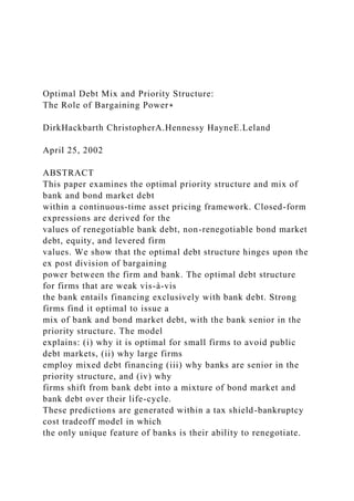
  • 32. EBPD depends on the existence of negotiation costs (δ > 0) and/or a BMD coupon commitment (c > 0). Intuitively, for EBPD default is triggered when equity is unwilling to pay the flow costs associated with servicing BMD and renegotiation costs that are necessary to maintain its claim on positive cash-flows in good states. Absent fixed costs associated with BMD and negotiation costs, default never occurs because equity incurs no flow cost in keeping alive its option. Of course, if renegotiation costs are sufficiently high, renegotiation does not occur. Additionally, for strong firms financing with a mixture of EBPD and BMD, renegotiation does not occur if c is sufficiently high relative to b. This is because for EBPD, the optimal renegotiation threshold Xs as given in (21) does not depend on c, whereas Xd increases monotonically in c. The following cases characterize the range of possible equilibria under EBPD: • For the firm financed exclusively with EBPD, if δ = 0, default never occurs. There exists an EBIT level Xs such that bs(X) = η (1−α)(1−τ)X on the interval (0, Xs) and bs(X) = b for all X ≥ Xs. This equilibrium is depicted in Figure 1.
  • 33. • If δ or c is positive, ∃ Xd such that equity declares default. • There is no renegotiation of EBPD for (δ,c) sufficiently high relative to b. • For positive δ or c, and (δ,c) sufficiently low relative to b, ∃ Xd such that default occurs endogenously; ∃ Xs > Xd such that bs(X) = η (1−α)(1−τ)X on (Xd, Xs) and bs(X) = b for all X ≥ Xs. This equilibrium is depicted in Figure 2. A.2. Bank Bargaining Power Debt With BBPD, in the event that equity fails to pay b and enters into renegotiation, it is the bank that makes take-it-or-leave it offers. In renegotiation, equity is pushed down to its reservation value, 13 which is zero under limited liability. Since equity value is everywhere zero on the renegotiation region, satisfaction of (2) implies the cash-flow to equity is zero in renegotiation states. That is, equity pays all free cash-flow, X−c, to the bank. So long as the bank is willing to service the BMD coupon commitment (c) as well as pay any negotiation costs, reorganization is avoided. Therefore, under BBPD, it is the bank that chooses when to enter into
  • 34. reorganization, whereas under EBPD it is equity that chooses when to enter into reorganization. The bank’s endogenous reorganization threshold under BBPD is denoted Xb(b,c). Lemma 1 proves that equity’s endogenous renegotiation threshold under BBPD for the mixed debt policy (b,c) is identical to the default threshold chosen by equity facing the BMD coupon commitment b + c. Intuitively, from the perspective of equity, there is no difference between default and entering into renegotiations with a bank that has full bargaining power, since both outcomes generate a claim worth zero. Lemma 1 For Bank Bargaining Power Debt, equity’s optimal switch point for entering into rene- gotiation satisfies Xs(b,c) = Xd(0,b+c). Proof. The cash-flow to equity in non-renegotiation states under BBPD for the pair (b,c) is identical to that under exclusive BMD finance with coupon ec = b + c. Default on BMD and renegotiation of the BBPD entail E[Xs(b,c)] = E[Xd(0,ec)] = 0. Result follows from the value matching and smooth pasting conditions being identical. To characterize the optimal financial structure of the firm in
  • 35. light of the distribution of bargain- ing power, the constituent pieces of the firm must be priced. The value of the marketable claims of the levered firm (v) is equal to the sum of the values of equity (E), bond market debt (C), and bank debt (B): v(X) = E(X)+C(X)+B(X). (23) Lemma 2 proves that the optimal financial policy for a weak firm that is able to issue BBPD entails financing with bank debt exclusively. This result holds regardless of the assumed values of the parameters (τ,α,δ,σ) and regardless of the assumed priority structure on any proposed mixed debt financing arrangement. 14 Lemma 2 For the Weak Firm, financing exclusively with Bank Bargaining Power Debt dominates any policy involving nonzero Bond Market Debt, regardless of priority structure. Proof. The optimal debt policy maximizes v. Consider an arbitrary mixed debt policy (b,c)
  • 36. with an arbitrary priority rule f that maps L to payments to the bank. Now consider the pure BBPD policy setting eb = b+c. From Lemma 2 it follows that the value of equity in the two firms is identical in all states. Let (es,eB) denote the bank debt service and bank debt value under pure BBPD finance. The mixed debt firm is represented by (s,B,C). Note that in non-reorganization states, es(X) = s(X) + c. On this same region, letting Φ be an indicator for renegotiation, flow renegotiation costs are identical for both firms and equal to Φ(X)δ[eb−es(X)]. The stopping time problem for the bank under pure BBPD is: eB(X0) ≡ max T E0 ·Z T 0 e−rt[es(Xt)−Φ(Xt)δ(eb−es(Xt))]dt+e−rTL(XT)¸ . The stopping time problem for the bank under mixed debt is: B(X0) ≡ max T E0 ·Z T 0 e−rt[s(Xt)−Φ(Xt)δ(b−s(Xt))]dt+e−rTf(L(Xt))
  • 37. ¸ . Let T∗ m ≡ inf{t ≥ 0 : Xt = Xb (b,c)} represent the optimal stopping time for the bank under mixed debt. Using the adding up constraint for recoveries in default, the equality of renegotiation costs, and the fact that es(X) = s(X)+ c in non-reorganization states we have: B(X0)+C(X0) = E0 "Z T∗ m 0 e−rt[es(Xt)−Φ(Xt)δ(eb−es(Xt))]dt+e−rT∗ mL(XT∗ m) # ≤ eB(X0). Lemma 2 suggests the following intuition for the dominance of pure BBPD finance over any mixed debt policy for weak firms. For any mixed debt policy (b,c), the firm can achieve the same equity valuation by issuing BBPD with couponeb = b+c. However, since it is the bank that decides when to terminate renegotiations, through its choice of Xb, it is optimal to avoid ex post inefficient bank decision rules that emerge when the choice of Xb generates an externality to other classes of debt. Similarly, BBPD dominates pure BMD finance since the option to remain open under
  • 38. BBPD has weakly positive value ex post. There is an alternative graphical interpretation regarding why pure BBPD dominates any mixed debt or pure BMD policy for weak firms. Assume that negotiation costs are zero. Consider 15 first the choice between issuing pure BMD versus pure BBPD when there are no negotiation costs. Assuming that the BMD policy entails coupon c, consider issuing BBPD with promised debt service b = c. Figure 3 depicts the debt service under BBPD. Note that the debt service under the BMD contract is represented by the horizontal segment. Clearly, the BBPD contract dominates since it entails higher tax shield benefits as well as lower bankruptcy costs. Figure 4 illustrates why BBPD dominates an arbitrary mixed debt policy entailing (b,c). The schedule beginning at Xb(b,c) > 0 depicts total debt service under the mixed policy. If the firm had financed with pure BBPD foreb = b+c no default would occur, implying bankruptcy costs are reduced. Further, additional tax shield benefits are realized, as the firm is able to shield income on the interval (0,Xb).
  • 39. Pricing of Bank Bargaining Power Debt Due to Lemma 2, in the remainder of the paper discussion of weak firms is confined to those financing exclusively with BBPD. We now solve for the price of BBPD and the bank’s optimal reorganization threshold Xb. The cash-flow to the bank in renegotiation states is equal to debt service, denoted by s(X), less renegotiation costs, if any: Cash-Flow to Bank = s(X)−δ[b−s(X)]+ (24) = ½ b for non-renegotiation states X −δ[b−X] for renegotiation states Below, we prove that an endogenous reorganization threshold for the bank does not exist if δ = 0. For δ > 0, the general solution for the value of BBPD is as follows: BL (X) = A3X a +A4X z + X(1+ δ) r−µ − δb r
  • 40. ∀ X ∈ [Xb,Xs) (25) BH (X) = A5X a +A6X z + b/r ∀ X ∈ [Xs,∞). (26) Based on Lemma 1, the optimal renegotiation point for equity (Xs) is derived below in (51), where the BMD model is solved. Taking Xs as given, the unknowns for this problem are (A3,A4,A5,A6,Xb) which are derived using the following boundary conditions: BL (Xb) = (1−α)V (Xb) , (27) ∂BL (Xb) ∂X = (1−α)V 0(Xb), (28) BL(Xs) = BH(Xs) (29) ∂BL (Xs) ∂X = ∂BH (Xs) ∂X (30) 16
  • 41. lim X→∞ BH (X) = b/r. (31) It is interesting to note that since it is the bank that chooses when to enter into reorganization, we have imposed value matching and smooth pasting conditions for the bank value function, with B pasting up smoothly to the reservation value function (R) at the point Xb. The solution is as follows:12 BL(X) = X(1+ δ) r−µ − δb r · 1− 1 (1−a) µ X Xb ¶a¸
  • 42. ∀ X ∈ [Xb,Xs) (32) BH (X) = · δb r(1−a) ¸· X Xb ¸a − · (1+ δ)b r(1−a) ¸· X Xs ¸a + b/r ∀ X ∈ [Xs,∞). (33) Xb = · δ δ + τ + α(1−τ)] ¸ Xs (34)
  • 43. = µ a 1−a ¶µ δb r ¶· δ + τ + α(1−τ) r−µ ¸−1 (35) Lemma 3 follows from inspection of the equation for Xb: Lemma 3 For Bank Bargaining Power Debt, ∃ Xb > 0 iff δ > 0. In terms of the optimal reorganization point, one can think of the bank as solving an optimal stopping problem which involves an irreversible switch from the stream of cash-flows associated with the BBPD to that associated with the reorganized firm. The reorganized firm generates the perpetual cash-flow (1−α)(1−τ)X. The difference in instantaneous cash-flows is:
  • 44. X[δ + τ + α(1−τ)]−δb. (36) The second expression for Xb embeds this cash-flow differential. In summary, the following cases characterize the range of possible equilibria under BBPD: • For the firm financed with BBPD, if δ = 0, default never occurs and∃ Xs such that s(X) = X on the interval (0, Xs) and s(X) = b for all X ≥ Xs. • If δ > 0, ∃ Xb such that the bank chooses to enter reorganization; ∃ Xs > Xb such that s(X) = X on (Xb, Xs) and s(X) = b for all X ≥ Xs. 12The expression for Xs is derived below in (51). 17 IV. Valuation of the Levered Firm Having characterized debt service functions for both EBPD and BBPD we can now solve for the constituent pieces of levered firm value. It is easily verified that the sum of instantaneous cash flows to equity, bond market debt, and bank debt is: Firm Cash Flow = (1−τ)X + τ[c+s(X)]−δ[b−s(X)]+. (37) This implies that the value of the levered firm can be expressed as the sum of the unlevered firm
  • 45. value, plus the value of the tax shield (TB), less negotiation costs (N), less bankruptcy costs (BC): v(X) = V (X) + TB(X) − N(X) − BC(X) (38) Before proceeding, the price of a particular primary claim will be of use for valuing a number of claims on the firm. Consider a primary claim paying $1 at the first-passage time from above of the EBIT process X to some threshold X∗ . Based on (2), it may be verified that for X ≥ X∗ , this claim’s value is: Hitting Claim = µ X X∗ ¶a (39) A. Tax Shield The value of the tax shield generated by bank and bond market debt is readily computed once one recognizes that the tax shield value is equal to the tax rate τ multiplied by the expected present value of future debt service. For the case of EBPD this latter value is equal to EBPD plus BMD
  • 46. less the creditors’ claims on recoveries in the event of default. To determine the value of the recovery claim held by the firm’s creditors, one multiplies the value of a hitting claim that pays off at Xd times the value of payoffs in default, L(Xd). Therefore, the tax shield value is: TB(X) = τ · C(X)+B(X)−L(Xd) µ X Xd ¶a¸ for EBPD. (40) The value of the tax shield in the case of BBPD is computed similarly, with negotiations costs, N(X), being added back to the value of the BBPD in order to compute the value of debt service: TB(X) = τ · B(X)+N(X)−L(Xb) µ X
  • 47. Xb ¶a¸ for BBPD. 18 B. Bankruptcy Costs For EBPD the deadweight loss in the event of default is given by αV (Xd). Therefore, we have the following expression for bankruptcy costs: BC(X) = αV (Xd) µ X Xd ¶a for EBPD. Similarly: BC(X) = αV (Xb) µ X Xb ¶a
  • 48. for BBPD. C. Negotiation Costs The negotiation cost function satisfies (2), with δ[b − s(X)] representing the flow term in the renegotiation region, while there is zero flow cost for X ≥ Xs. The following boundary conditions pin down the solution for EBPD. For BBPD, one simply replaces Xd with Xb in the first boundary condition. NL (Xd) = 0, (41) NL (Xs) = NH (Xs) , (42) ∂NL (Xs) ∂X = ∂NH (Xs) ∂X , (43) lim X→∞ N (X) = 0. (44) For EBPD the solution for the negotiation cost function is: NL(X) = δ b
  • 50. −δ µ η (1−α)(1−τ) r−µ ¶· X − µ Xd − µ a−1 a−z ¶ Xs µ Xd Xs ¶z¶µ X Xd ¶a − µ a−1 a−z ¶ Xs
  • 53. µ 1−z a−z ¶ Xs µ X Xs ¶a¸ For BBPD the solution for the negotiation cost function is: NL(X) = δ b r · 1− µ 1− µ a a−z ¶µ Xb Xs ¶z¶µ X
  • 58. D. Bond Market Debt Value The value function for bond market debt satisfies (2) with flow payment equal to c on the non- default region. The boundary conditions are value matching at Xd, and an asymptotic condition: C (Xd) = (1−η)(1−α)V (Xd), (49) lim X→∞ C (X) = c/r. (50) The solution for the value of BMD is given by: C(X) = c r · 1− µ X Xd ¶a¸ +(1−η)(1−α)V (Xd) µ X
  • 59. Xd ¶a (51) E. Equity Value Finally, having derived each of the terms in the levered firm value expression (38), the value of equity can be expressed as a residual based on (23). In the case of EBPD, the following valuation equation holds on the interval [Xd,∞) : E(X) = V (X)−V (Xd) µ X Xd ¶a −(1−τ) · B(X)+C(X)−L(Xd) µ X Xd ¶a¸ −N(X) for EBPD. (52) In the case of BBPD, equity is worth zero for X ≤ Xs, since it is
  • 60. pushed down to its reservation value in renegotiations. The following pricing equation holds on the interval (Xs,∞) : E(X) = V (X)−V (Xb) µ X Xb ¶a − (1−τ) · B(X)+N(X)−L(Xb) µ X Xb ¶a¸ for BBPD. The two expressions for the value of equity under EBPD and BBPD have intuitive interpretations. The first two terms represent the value of holding an unlevered firm that will be worthless at the first-passage of the EBIT process to the relevant reorganization threshold. The third term represents the expected present value of the after-tax cost of total debt service. The fourth term
  • 61. 20 is renegotiation costs, which is paid by equity in the case of EBPD but is paid by the bank in the case of BBPD. The remaining unknown variable for the case of EBPD is the optimal default threshold, Xd(b,c). The brute force method of solving for equity value and the endogenous default threshold is to solve for the flow payments to equity and then utilize the following boundary conditions: EL(Xd) = 0 (53) EL(Xs) = EH(Xs) (54) ∂EL (Xs) ∂X = ∂EH (Xs) ∂X (55) lim X→∞ E (X) =
  • 62. (1−τ)X r−µ − (1−τ)(b+c) r (56) ∂EL (Xd) ∂X = 0 (57) However, it can be verified that the solution (52) necessarily satisfies the first four boundary con- ditions. The smooth pasting condition at default must therefore be exploited in solving for Xd. Using (21), the endogenous default-triggering EBIT level under an arbitrary mixture of EBPD and BMD is: Xd(b,c) = a(r−µ)[δb+(1−τ)c] (a−1)r(1−τ)[1−η (1−α)(1−τ −δ)] (58) V. Optimal Debt Structure under Mutually Exclusive Financing A. Analysis of Strong Firm A.1. Bond Market Debt Finance We begin with an analysis of the bond market debt financed
  • 63. firm, confirming that the qualitative features of the Leland (1994) framework carry over to our model. The discussion will be brief, since the main objective of this section is to contrast the bond market and bank debt firms. Dropping terms in (38) that involve bank debt, the expression for the value of the marketable claims of the corporation is given by: v(X) = V (X)+ τc r µ 1− µ X Xd ¶a¶ −αV (Xd) µ X Xd ¶a . (59)
  • 64. 21 Value matching and smooth pasting conditions for equity yield the following solution for the en- dogenous default-triggering EBIT level as a function of the promised coupon payment: Xd(0,c) = µ r−µ r ¶ µ a a−1 ¶ c. (60) Differentiating the previously derived expression for the value of bond market debt given in (51), with respect to c and setting it equal to zero yields the bond market debt coupon capacity, denoted cmax: cmax (X0) = r(a−1)X0 a(r−µ) [1−a(τ + α(1−τ))]
  • 65. 1/a . (61) Substituting this expression back into the pricing equation yields the bond market debt value ca- pacity: Cmax (X0) = X0 [1−a(α +(1−α)τ)]1/a (r−µ) . (62) Figure 5 parallels Figure 1 in Leland (1994) presenting comparative statics results for the value of bond market debt as a function of leverage for varying degrees of underlying cash flow risk. It is easy to see that a debt capacity cmax obtains. Perhaps surprisingly, it can be seen that the firm’s bond market debt coupon capacity is increasing in EBIT risk, but the bond market debt value capacity decreases in the riskiness of the underlying cash flows. We can compute the optimal coupon by solving the first-order condition ∂v(X0;c∗ )/∂c = 0: c∗ (X0) = r(a−1)X0 a(r−µ) · τ −a(τ + α(1−τ))
  • 66. τ ¸1/a (63) Substituting this expression back into the total firm value expression yields the ex ante value of an optimally levered bond market debt firm: v∗ (X0;0,c∗ ) = X0 r−µ ( 1−τ + τ · τ −a(τ + α(1−τ)) τ ¸1/a) (64) Figure 6 depicts the optimal coupon level c∗ . Although high volatility firms have a higher debt coupon capacity than low volatility firms, the optimal choice of leverage goes in the opposite direction in that it is greater for low volatility firms than it is for high volatility firms. Altogether, less risky firms attain a higher total levered firm value by
  • 67. issuing a higher promised coupon level relative to riskier firms. 22 A.2. Equity Bargaining Power Debt Finance We begin this subsection by verifying that some of the key results in MBP (1997) relating to the case in which equity has full bargaining power are also valid in our modeling framework. Lemma 4 If c = δ = 0, the Strong Firm financing with EBPD never defaults. Proof. Follows from the fact that default is not optimal when the cash-flow to equity is everywhere positive. Lemma 5 For the Strong Firm, if τ = 0, δ = 0, and α > 0, then the optimal financial structure entails no Bond Market Debt, and the firm is indifferent regarding the level of b. Proof. Issuing BMD entails default costs, whereas EBPD entails no such costs. Lemma 6 For the Strong Firm, if δ = 0 and τ > 0, it is optimal to increase b up to the bank debt
  • 68. capacity, bmax, which satisfies B[X0;bmax] = L(X0). The ex ante firm value for any b ≥ bmax is V (X0)[1+ τ(1−α)]. Proof. Since there are no negotiation costs and default never occurs, the firm solves the problem max b τB[X0;b]. The intuition for bank debt capacity in this setting is as follows. From the equation for the endogenous renegotiation threshold given in (21), it can be seen that Xs is increasing in b. For a fixed initial EBIT level, low levels of b are consistent with X0 > Xs(b). However, for b sufficiently high, the bank recognizes that equity will push it down to the reservation value L(X0) immediately, assuming equity has maximum bargaining power. This implies that increasing the promised coupon will not raise the value of debt, since the reservation value is invariant to b. More formally, the bank debt capacity, bmax, satisfies: Xs (b max) = X0 ⇔bmax = µ
  • 69. r r−µ ¶ µ a−1 a ¶ (1−α) (1−τ) X0. (65) We now proceed to a discussion of some numerical results. Figure 7 depicts the bank’s reservation value R and the value of bank debt B as functions of EBIT for varying levels of bankruptcy costs, 23 assuming that equity has full bargaining power. In the model, the strategic debt service to the bank in the renegotiation region depends crucially on the level of bankruptcy costs (and corporate taxes, for which the effect is essentially the same). The dashed rays from the origin represent the bank’s threat point or, more formally, reservation value function R(α, ·). The construction of the incentive compatible switch point Xs(α, ·) implies that the bank debt value B is tangent to R(α, ·) up to Xs(α, ·). Note that ceteris paribus, firms with higher bankruptcy costs enter negotiations
  • 70. with their bank sooner. The figure clearly depicts the fact that the bank is pushed down to its reservation value in the renegotiation region, where B(X) = R(X), with value matching and smooth pasting being exhibited at Xs. Figure 8 depicts the value of EBPD (B) and BMD (C) as functions of EBIT (X) evaluated at the same promised coupon, b = c = 20 in the presence of negotiation costs. Note that default occurs earlier with BMD than with EBPD. However, for points to the right of Xd, the value of BMD exceeds that of EBPD. Figure 9 reports comparative static results for the price of bank debt when the firm’s EBIT volatility varies. EBPD is worth weakly more when the firm’s operations are less risky. This is not surprising given that in Figure 7 it was shown that EBPD is concave in EBIT. It is also interesting to note that the higher the underlying volatility, the longer the firm waits before entering into renegotiation. Figures 10-12 explore some comparative statics for the effects of key parameters on the total leveraged firm value v. Lemma 6 demonstrated that with δ = 0, it is optimal for the firm to lever
  • 71. up to its debt capacity. Figure 10 illustrates the effect variations in negotiation costs. It can be seen that the introduction of negotiation costs generates an interior optimal coupon, with higher negotiation costs implying a lower firm value and a lower optimal coupon b∗ . Figure 11 depicts the effect of variations in bankruptcy costs. It can be seen that the firm’s debt capacity and optimal coupon are inversely related to bankruptcy costs. In other words, the model predicts that firms with lower bankruptcy cost have more access to bank debt and will optimally choose to borrow more. Figure 12 indicates that firm value is decreasing in underlying cash flows’ volatility. Finally, the effect of an increase in perpetual coupon payments from b = 10 to b̃ = 15 on strategic debt service is illustrated in Figure 13. Provided negotiation costs are strictly positive, an increase in the promised coupon: (i) shifts the default-triggering EBIT level up ∂Xd (b,0)/∂b > 0; (ii) 24
  • 72. results in a loss in tax shield benefits in the region between the previous switch point Xs and the new switch point X̃ s > Xs; and (iii) brings about an increase in tax shield benefits in the non- renegotiation region, i.e., for all X ∈ [X̃ s,∞). This provides the underlying basis for the interior optimum b∗ . A.3. Equity Bargaining Power and Bond Market Debt Comparison The purpose of this section is to compare EBPD and BMD, when the choice between the two is mutually exclusive.13 We begin by comparing EBPD and BMD when the firm may choose the optimal coupon commitment for each, respectively. Under the base case parameter values there exist threshold values of bankruptcy costs α∗ and corporate taxes τ∗ at which the firm is indifferent between EBPD and BMD. Figure 14 reports valuations applicable to optimally levered EBPD and BMD firms as α is varied. For the optimal promised coupon payments b∗ (α, ·) and c∗ (α, ·) , firms with bankruptcy costs of 31% or less prefer EBPD. At first the result may seem counter-intuitive. After all, casual intuition suggests that issuing a hard claim like BMD is less attractive when
  • 73. bankruptcy costs increase. There is nothing wrong with this intuition, as far as it goes. That is, an increase in α reduces the optimal coupon commitment under BMD and the total firm value attained. However, increases in bankruptcy costs also make EBPD less attractive and lower the value attained. As Lemma 6 demonstrates, this effect is present even when the issuance of EBPD entails no default (when δ = 0). This is because increases in α reduce the value of the tax shield created by EBPD. Recall that under EBPD, the bank is pushed down to its reservation value in renegotiations. Increases in α rotate the function R clockwise downwards, implying lower debt service under EBPD. Figure 15 reports valuations applicable to optimally levered EBPD and BMD firms as τ is varied. At the promised coupon levels b∗ (τ, ·) and c∗ (τ, ·) firms with corporate taxes of less than 26% achieve a higher value with bank debt. Finally, Figure 16 traces out the locus of points at which the firm is indifferent between the two sources of capital so long as they are mutually 13This case would be of particular interest when there are substantial fixed costs associated with tapping either
  • 74. source of debt capital. 25 exclusive. If δ = 0, the following condition identifies parameters such that EBPD dominates BMD, when both are optimally levered: (1−α)(1−τ) > {1−a [τ + α(1−τ)]/τ}1/a . (66) Finally, by parametrically varying the firm’s EBIT volatility another empirical prediction emerges. In line with previous theoretical and empirical studies, we obtain the result that safer firms find it optimal to tap public debt markets, while riskier firms are more likely to be financed by banks. Turning now to the analysis of equal promised coupon payments to the bank and the bond market, Figures 17—19 confirm in principle all of the previous findings for optimally levered firms. Assuming that δ = 0, we can derive an analytic expression for the cut-off contour under equal promised payments to EBPD and BMD. The following condition defines parameter values such that the EBPD financed firm with the same perpetual coupon
  • 75. promise as the BMD firm achieves higher value (when both are evaluated at X > Xs): [(1−α)(1−τ)]−a > (1−a)1/a. (67) Figure 19 confirms the intuition that ceteris paribus bank debt is more desirable for lower nego- tiation costs δ; that is, a decrease in the negotiation costs δ implies that more (α,τ) pairs lead to the optimality of EBPD for mutually exclusive financing decisions. B. Analysis of Weak Firm This section presents numerical results for the weak firm. We confine analysis to issuance of BBPD, since for a weak firm the issuance of BMD is dominated, as was shown in Lemma 2. To begin, we parallel the analysis of EBPD by plotting BBPD as a function of EBIT when the cost of negotiation with the bank changes (Figure 20) and when the firm’s cash flow riskiness varies (Figure 21). It is important to note that under BBPD, the bank becomes the residual claimant on the firm’s cash flows in the renegotiation region. The value function for BBPD therefore pastes smoothly to the reservation function R at the endogenous
  • 76. reorganization threshold Xb. Figure 21 illustrates that for any positive negotiation costs (δ > 0) both the default-triggering EBIT level Xb and the incentive compatible switch point Xs are decreasing in the firm’s riskiness σ. Also, the value function for BBPD exhibits a convex-concave shape, illustrating that the bank also becomes risk-loving in some states. 26 As was already noted, under BBPD the bank becomes the residual claimant in the renegotiation region. The has an important implication for the equity value function, which is depicted in Figure 22. In particular, the value of equity is equal to zero in the renegotiation region since the bank pushes equity down to its reservation value. At equity’s incentive compatible switch point for entering into renegotiations (Xs), the equity value function exhibits value-matching and smooth- pasting. Figure 23 illustrates that lower negotiation costs generate a higher optimal coupon under BBPD.
  • 77. Figure 24 indicates that the value attained by the optimally levered firm is higher when the volatility ofunderlyingEBITis reduced. TheeffectofvolatilityonfirmvalueunderBBPDseemsqualitatively similar to the results reported in Figure 5 for firm value under BMD. However, it is interesting to note that the increase in firm value stemming from lower volatility is achieved via different means, depending on the type of debt issued. For BMD, the optimal coupon commitment increases when volatility is reduced. For BBPD, on the other hand, the optimal coupon commitment decreases when volatility is reduced. VI. Optimal Debt Structure of the Mixed Debt Firm This section confines discussion to the case of the strong firm since Lemma 2 demonstrates that the optimal debt structure for the weak firm entails exclusive BBPD financing. We begin with an analysis of the optimal mix of EBPD and BMD when the bank is placed senior in the priority structure. Analysis of pari passu treatment follows. Comparison of ex ante firm valuations achieved under the optimal debt mix for each priority rule,
  • 78. respectively, pins down the optimal priority structure. A. Senior Bank Debt The following result is useful before proceeding to the numerical results for senior bank debt. Lemma 7 For a Strong Firm issuing the mixed debt pair (b,c) such that there is no renegotiation region, the ex ante firm value is equivalent to that under BMD finance with ec = c+ b. 27 Proof. If there is no renegotiation, then bank debt represents a hard claim from the perspective of equity, implying that the optimal default threshold is based upon facing a fixed flow cost c + b at each instant. This is the same situation facing a firm that has promised ec = c+ b to the bond markets. Intuitively, no renegotiation region exists when the bank is senior and the debt mix is weighted heavily towards BMD. In such cases: R[Xd(b,c)] = (1−α)(1−τ)Xd(b,c)
  • 79. r−µ > b r , (68) implying that no renegotiation occurs, since the bank rejects any debt service payment less than b. Therefore, full analysis of levered firm valuations for the strong firm is conducted as follows. Senior bank debt is examined by setting η = 1 and solving the model for parameters (b,c) are such that there exists a renegotiation region. Other (b,c) pairs are subsumed under the exclusive BMD financing case. The analysis of the model in this subsection has been accompanied by several consistency checks of the numerical scheme. First, the theoretical results for the pricing of claims for the mixed-debt firm are predicated on the assumption that there exists a non-trivial renegotiation region. Therefore, we need to impose the following regularity condition in our numerical analysis of the mixed debt firm: Condition 1: Xd (b,c, ·) < Xs (b, ·) ∀ (b,c) ∈ IR2+ (69)
  • 80. Secondly, it was stated that for certain (b,c) pairs the firm may be in the position to issue safe, senior bank debt. These cases are subsumed in the analysis of the BMD firm. To avoid any pathological cases, the numerical scheme consequently needs to contain a second regularity condition for the mixed debt firm: Condition 2: L [Xd (b,c, ·)] < b/r ∀ (b,c) ∈ IR2+ (70) Figures 25 indicates that for the strong firm there exists an interior optimum debt mix (b∗ ,c∗ ) = (24.09,23.63), when the bank is senior in the priority structure. Although the promised coupon to the bank is higher, the initial value of BMD (334.94) exceeds that on EBPD (315.31). Regardless of the measure, the optimal debt mix when the bank is senior is relatively even. Substantial increases in firm value are achieved when the firm can exploit a mix of EBPD and BMD, rather than relying 28 on one source exclusively. The first line below reports the ex ante firm value attained when the
  • 81. firm may mix EBPD and BMD, assuming the bank is senior. The second and third lines report valuations under exclusive BMD and EBPD finance, respectively: v (b∗ ,c∗ ) = 844.09 (71) v(c∗ ) = 809.30 v(b∗ ) = 752.01. An interesting feature of the model is that it may be used to generate estimates regarding the magnitude of the benefit the firm enjoys when it gains access to a previously untapped source of funds. The results above indicate that firms without access to the bond markets reap large gains when this constraint is removed. Note that this result holds in the absence of any notion that bond markets are “cheaper.” In this model all claims are priced fairly, with all claimants discounting flows at the rate r. All of the benefit from mixed debt finance comes from the complementarity effect. Firm value increases by 4.3% when mixed debt is employed, rather thanfinancing exclusively with BMD. The increase in firm value is 12.2% when mixed debt is employed, rather than financing
  • 82. exclusively with EBPD. The complementarity effect is due the relationship between bank and bond market debt coupon payments and the default-triggering EBIT level Xd (b,c, ·). Therefore, we fix the default-triggering EBIT level at Xd (b,c, ·) = 5 in Figure 33 and solve for the (b,c) pairs such that our root equation is satisfied. This analysis reveals that bank and bond market debt have an uneven contribution to the endogenous bankruptcy boundary and hence a complementarity effect of the nature discussed above obtains. Secondly, in comparing these numerical results, it can be seen that placing bank debt senior in the priority structure leads to higher total firm value. Lastly, at a broader level these findings show that our model yields a product differentiation result for financial markets in the following sense. In order to maximize firm value, the role of banks is to issue genuinely soft debt such that they offer a financial product, which is as “distant” as possible from hard bond market debt. Thus we provide a rationale for the coexistence of bank debt (indirect/intermediated finance) and bond market debt (direct finance).14 14See for instance Bolton and Freixas (2000) for a similar
  • 83. result. These authors obtain coexistence of bank and bond market debt from an asymmetric information model of financial intermediation. 29 The individual value components of the total leveraged firm are reported in Figures 27—32. Valuations for bank B and bond market debt C are depicted as functions of coupon payments to the bank b and to the bond market c in Figures 31 and 32, respectively. Our earlier discussion on comparative statics results concerning debt capacity of the all soft (hard) debt firm are confirmed by these graphs. B. Equal Priority Bank Debt The following result will be useful before proceeding to the numerical results for the case of equal priority bank debt. Lemma 8 Under equal priority with endogenous default, it is impossible for the firm to issue safe EBPD or BMD. Proof. Suppose to the contrary that either class is safe. Then it must be the case that
  • 84. L[Xd(b,c)] ≥ b+cr and there is no renegotiation. With no renegotiation the endogenous default threshold is the same as that pertaining to a firm issuing bond market debt exclusively, with promised payment ec = c+b. But L[Xd(0,ec)] < ecr. This is a contradiction. Corollary 9 A renegotiation region always exists for the Strong Firm issuing equal priority EBPD. Figure 26 indicates that for the strong firm there exists an interior optimum debt mix (b∗ ,c∗ ) = (5.89,32.53), when the bank is pari passu in the priority structure. However, the debt mix is slanted towards BMD under pari passu, whereas it was roughly equal for senior bank debt. More modest increases in firm value are achieved when the firm can exploit a mix of EBPD and BMD, rather than relying on one source exclusively. The first line below reports the ex ante firm value attained when the firm may mixes EBPD and BMD, when the bank is pari passu. The second and third lines report valuations under exclusive BMD and EBPD finance, respectively: v (b∗ ,c∗ ) = 816.15 (72) v(c∗ ) = 809.30
  • 85. v(b∗ ) = 752.01 30 Under equal priority, firm value increases by 0.8% when mixed debt is employed, rather than financing exclusively with BMD. The increase in firm value is 8.5% when mixed debt is employed, rather than financing exclusively with EBPD. For our baseline parameter values, placing the bank senior in the priority structure dominates pari passu, with the ex ante firm values equal to 844.09 and 816.15, respectively. The increase in firm value associated with moving away from pari passu is 3.4%. Why does placing the bank senior generate superior ex ante firm valuations? Table 1 suggests an answer. Placing the bank senior in the priority structure offers costs and benefits relative to pari passu treatment. On the one hand, placing the bank senior leads to an increase in bankruptcy costs equal to 4.78. The increase in bankruptcy costs is generated by the increase in the optimal default threshold from 8.11 to 8.76. The optimal default
  • 86. threshold increases because placing the bank senior raises the bank’s threat point in instantaneous negotiations, leading to higher requisite debt service. Outweighing this cost is the benefit of high ex post debt service in terms of combined tax shield increases and renegotiation cost reductions. Most of the benefit is generated by the increase in the value of the tax shield, which increases in value by 32.27 when the bank is placed senior in the priority structure. 31 VII. Conclusions/Extensions • Non-linear tax schedule. • Agency problems, e.g. endogenous volatility as in Leland (1998). • Costly monitoring by banks. • Monitoring of bank debt. • Maturity structure, as in Leland and Toft (1996). 32
  • 87. References Anderson, Ron W. and Suresh M. Sundaresan, 1996, The design and valuation of debt contracts, Review of Financial Studies 9, 37—68. Andrade, Gregor and Steven N. Kaplan, 1998, How costly is financial (not economic) distress? Evidence from highly leveraged transactions that became distressed, Journal of Finance 53, 1443— 1493 Asquith, Paul, Robert Gertner, and David Scharfstein, 1994, The anatomy of financial distress: An examination of junk bond issuers, Quarterly Journal Economics 109, 625—658. Barclay, Michael J. and Clifford W. Smith, Jr., 1995a, The maturity structure of corporate debt, Journal of Finance 50, 609—631. Barclay, Michael J. and Clifford W. Smith, Jr., 1995b, The priority structure of corporate liabilities, Journal of Finance 50, 899—917. Berglöf, Erik, and von Thadden, Ernst-Ludwig, 1994, Short- term versus long-term interests: Cap- ital structure with multiple investors, Quarterly Journal Economics 109, 1055—1084. Black, Fischer, 1975, Bank funds management in an efficient market, Journal of Financial Eco- nomics 2, 323—339. Black, Fischer and John C. Cox, 1976, Valuing corporate
  • 88. securities: Some effects of bond indenture provision, Journal of Finance 31, 351—367. Bolton, Patrick, and Xavier Freixas, 2000, Equity, bonds, and bank debt: Capital structure and financial market equilibrium under asymmetric information, Journal of Political Economy 108, 324—342. Bolton, Patrick, and Scharfstein, David S., 1996, Optimal debt structure and the number of credi- tors, Journal Political Economics 104, 1—25. Carey, Mark, 1995, Are bank loans mispriced? Mimeo, Board of Governors of the Federal Reserve System. Chemmanur, Thomas J. and Paolo Fulghieri, 1994, Reputation, renegotiation, and the choice between bank loans and publicly traded debt, Review of Financial Studies 7, 475—506. Diamond, Douglas W., 1991, Monitoring and reputation: The choice between bank loans and directly placed debt, Journal of Political Economy 99, 688— 721. Diamond, Douglas W., 1993a, Seniority and maturity of debt contracts, Journal of Financial Economics 33, 341—368. Diamond, Douglas W., 1993b, Bank loan maturity and priority when borrowers can refinance, in: Capital Markets and Financial Intermediation (Colin Mayer and Xavier Vives, Eds.). Cambridge University Press.
  • 89. Dumas, Bernard, 1991, Super Contact and Related Optimality Conditions, Journal of Economic Dynamics and Control 15, 675—685. 33 Fama, Eugene F., 1985, What’s different about banks?, Journal of Monetary Economics 15, 29—40. Fama, Eugene F., 1990, Contract costs and financing decisions, Journal of Business 63, 571—591. Fan, Hua, and Suresh M. Sundaresan, 2000, Debt valuation, renegotiation, and optimal dividend policy, Review of Financial Studies 13, 1057—1099. Franks, Julian, and Walter N. Torous, 1989, An empirical investigation of U.S. firms in reorgani- zation, Journal of Finance 44, 747—769. Franks, Julian, and Walter N. Torous, 1994, A comparison of financial recontracting in distressed exchanges and chapter 11 reorganizations, Journal of Financial Economics 35, 349—370. Gertner, Robert and David Scharfstein, 1991, A theory of workouts and and the effect of reorgani- zation law, Journal of Finance 46, 1189—1122. Giammarino, Ronald, 1989, The resolution of financial distress, Review of Financial Studies 2, 25—47.
  • 90. Goldstein, Robert, Nengjiu Ju, and Hayne E. Leland, 2001, An EBIT-Based Model of Dynamic Capital Structure, Journal of Business 74, 483—512. Hackbarth, Dirk, and Hayne E. Leland, 2001, Capital Structure with Multiple Classes of Debt, Mimeo, University of California, Berkeley. Harrison, J. Michael, 1985, Brownian Motion and Stochastic Flow Systems, Wiley Press. Hart, Oliver and John H. Moore, 1995, Debt and seniority: An analysis of the role of hard claims in constraining management, American Economic Review 85, 567—585 Hart, Oliver and John H. Moore, 1998, Default and renegotiation: A dynamic model of debt, Quarterly Journal of Economics 103, 1—41. Kahl, Matthias, 2001, Financial distress as a selection mechanism: Performance and survival from the onset to the resolution of financial distress, Mimeo, University of California, Los Angeles. Kose, John, 1993, Managing financial distress and valuing distressed securities: A survey and a research agenda, Financial Management Autumn, 60—78. Leeth, John and Jonathan Scott, 1989, The incidence of secured debt: Evidence from the small business community, Journal of Financial and Quantitative Analysis 24, 379—394. Leland, Hayne E., 1994, Corporate debt value, bond covenants and optimal capital structure,
  • 91. Journal of Finance 49, 1213—252. Leland, Hayne E. and Klaus B. Toft, 1996, Optimal capital structure, endogenous bankruptcy, and the term structure of credit spreads, Journal of Finance 51, 987—1019. Leland, Hayne E., 1988, Agency costs, risk management and capital structure, Journal of Finance 53, 1213—1243. Mann, Ronald J., 1997, The role of secured credit in small- business lending, Mimeo, Washington University School of Law. Mayer, Colin, 1988, New issues in corporate finance, European Economic Review 32, 1167—1188. 34 Mella-Barral, Pierre, and William Perraudin, 1995, Strategic Debt Service, Journal of Finance 52, 531—556. Merton Robert C., 1974, On the pricing of corporate debt: The risk structure of interest rates, Journal of Finance 29, 449—470. Morris, Stephen and Hyun S. Shin, 2001, Coordination risk and the price of debt, Mimeo, London School of Economics & Political Science. Park, Cheol, 2000, Monitoring and structure of debt contracts, Journal of Finance 55, 2157—2195.
  • 92. Petersen, Mitchell A., and Rajan, Raghuram G., 1995, The effect of credit market competition on lending relationships, Quarterly Journal of Economics. 110, 407—443. Rajan, Raghuram G., 1992, Insiders and outsiders: The choice between informed and arm’s length debt, Journal of Finance 47, 1367—1400. Ross, Michael, 1997, Dynamic optimal risk management and dividend policy under optimal capital structure and maturity, Mimeo, University of California, Berkeley. Schwartz, Alan, 1997, Priority contracts and priority in bankruptcy, Cornell Law Review 82, 1396— 1435. Scott, James A., Jr., 1977, Bankruptcy, secured debt, and optimal capital structure, Journal of Finance 32, 1—19. Smith, Clifford W., Jr., and Jerold B. Warner, 1979, Bankruptcy, secured debt, and optimal capital structure: Comment, Journal of Finance 34, 247—251. Summers, Lawrence H. and David M. Cutler, 1988, The costs of conflict resolution and financial distress: Evidence from the Texaco-Pennzoil litigation, Rand Journal of Economics 19, 157—172. Welch, Ivo, 1997, Why is bank debt senior? A theory of asymmetry and claim priority based on influence costs, Review of Financial Studies 10, 1203—1236.
  • 93. Winton, Andrew, 1995, Costly state verification andmultiple investors: The roleof seniority, Review of Financial Studies 8, 91—123. 35 T a b le I C o m p a r is o n o f O p ti m a l D e b t a
  • 123. ³³³ b Figure 1: Strategic debt service s(X) as a function of EBIT X in case of Equity Bargaining Power Debt (EBPD). It is assumed that there are no negotiation costs (δ = 0). 37 - X 6 s(X) c : : : : : : : : : :. s Xs
  • 124. ³³ ³³ ³³ ³ s: : Xd b Figure 2: Strategic debt service s(X) as a function of EBIT X in case of Equity Bargaining Power Debt (EBPD). It is assumed that either there are negotiation costs (δ > 0) or the firm issued Bond Market Debt (c > 0). Note that for positive δ or c, and (δ,c) sufficiently low relative to b, ∃ Xd(b,c;δ) such that default occurs endogenously and a nontrivial renegotiation region exists: Xd(b,c;δ) < Xs. 38 - X 6 s(X) c :
  • 125. : : : s Xd(0,c) ¡ ¡ ¡ ¡ ¡ ¡ ¡ ¡¡ b = c Figure 3: Strategic debt service s(X) as a function of EBIT X in case of Bank Bargaining Power Debt (BBPD). It is assumed that there are no negotiation costs (δ = 0) and that the promised coupon payments under Bank Bargaining Power Debt and Bond Market Debt are identical: b = c. Note that the defaul- triggering EBIT level under BMD is equal to the switch point under BBPD, i.e., Xd(0,c) = Xs(b). 39 - X
  • 127. Xb(b,c) Figure 4: Strategic debt service s(X) as a function of EBIT X in case of Bank Bargaining Power Debt b̃ = b+c versus strategic debt service of a mixed debt firm financed by Bank Bargaining Power Debt b and Bond Market Debt c. Note that the incentive compatible switch point Xs is the same under both debt structures, but the latter is associated with a strictly positive default point Xb(b,c). It is assumed that there are no negotiation costs (δ = 0). 40 0 20 40 60 80 100 c 0 200 400 600 800 C cmax
  • 128. Figure 5: Bond market debt value C as a function of promised coupon payments c when the firm’s EBIT volatility varies: σ = 10% (long-dashed line), σ = 20% (solid line), and σ = 30% (short-dashed line). It is assumed X0 = 20, r = 6%, µ = 4%, α = 50%, τ = 35%, η = 0. Note that the hard debt capacity cmax depends on firm’s riskiness σ. Cf. Figure 1 in Leland (1994). 41 0 20 40 60 80 c 650 700 750 800 850 900 v c* Figure 6: Total firm value v of a Bond Market Debt firm as a function of promised coupon payments c when EBIT volatility varies: σ = 10% (long-
  • 129. dashed line), σ = 20% (solid line), and σ = 30% (short-dashed line). It is assumed X0 = 20, r = 6%, µ = 4%, α = 50%, τ = 35%, η = 0. Note that the optimal leverage c∗ depends on firm’s riskiness σ. Cf. Figure 6 in Leland (1994). 42 0 10 20 30 40 50 X 50 100 150 200 250 300 350 400 B dna R Xs
  • 130. Figure 7: Equity Bargaining Power Debt B and bank’s reservation value R as a function of EBIT X for a given coupon level b as the firm’s bankruptcy costs vary: α = 25% (long dashed line), α = 50% (solid line), and α = 75% (short-dashed line). It is assumed that X0 = 20, b = 20, r = 6%, µ = 4%, σ = 20%, τ = 35%, δ = 0, η = 1. Note that both the bank’s reservation value R (thin short- dashed lines) and the incentive compatible switch point Xs depend on the firm’s bankruptcy costs α. 43 0 10 20 30 40 50 X 50 100 150 200 250 300 350 400
  • 131. B dna C Xd Xs Figure 8: Equity Bargaining Power Debt B as a function of EBIT X for a given coupon level b. It is assumed that X0 = 20, b = 20, r = 6%, µ = 4%, σ = 20%, α = 50%, τ = 35%, δ = 10%, η = 1. The Bond Market Debt C as a function of EBIT X for the same coupon level b = c is depicted by the dashed line. Note that ceteris paribus default occurs earlier with Bond Market Debt than with Equity Bargaining Power Debt. 44 0 10 20 30 40 50 X 50 100 150 200 250 300
  • 132. 350 400 B =Xd Xs Figure 9: Equity Bargaining Power Debt B as a function of EBIT X for a given coupon level b as EBIT volatility varies: σ = 10% (long-dashed line), σ = 20% (solid line), and σ = 30% (short-dashed line). It is assumed X0 = 20, b = 20, r = 6%, µ = 4%, α = 50%, τ = 35%, δ = 0%, η = 1. Note that the default- triggering EBIT level Xd is equal to zero in all cases because the negotiation cost δ is equal to zero, but the incentive compatible switch point Xs still varies with the firm’s riskiness σ. 45 0 5 10 15 20 25 b 680 700 720 740
  • 133. 760 v bmaxb* Figure 10: Total firm value v of an Equity Bargaining Power Debt firm as a function of promised coupon b when the firm’s negotiation cost varies: δ = 10% (long-dashed line), δ = 20% (solid line), and δ = 30% (short-dashed line). It is assumed X0 = 20, r = 6%, µ = 4%, σ = 20%, α = 50%, τ = 35%, η = 1. Note that optimal leverage b∗ depends on the size of negotiation costs δ, but not the firm’s debt capacity bmax. 46 0 10 20 30 40 b 680 700 720 740 760 780
  • 134. 800 v bmaxb* Figure 11: Total firm value v of an Equity Bargaining Power Debt firm as a function of promised coupon b when the firm’s bankruptcy costs vary: α = 25% (long dashed line), α = 50% (solid line), and α = 75% (short-dashed line). It is assumed that X0 = 20, r = 6%, µ = 4%, σ = 20%, τ = 35%, δ = 10%, and η = 1. Note that both optimal leverage b∗ and debt coupon capacity bmax depend on the firm’s bankruptcy costs α. 47 0 5 10 15 20 25 30 35 b 660 680 700 720 740
  • 135. 760 v b bmaxb* bmaxb* bmaxb* bmax Figure 12: Total firm value v of an Equity Bargaining Power Debt firm as a function of promised coupon b when the firm’s EBIT volatility varies: σ = 10% (long-dashed line), σ = 20% (solid line), and σ = 30% (short-dashed line). It is assumed X0 = 20, r = 6%, µ = 4%, α = 50%, τ = 35%, δ = 10%, η = 1. Note that both optimal leverage b∗ and debt capacity bmax depend on the firm’s riskiness σ. 48 0 5 15 20 X 2 4 6 8 10 12
  • 136. 14 s Xd X ~ d Loss Loss Gain Xs X ~ s Figure 13: “Loss” versus “Gain” of bank debt’s strategic service flow s with equity making take-it-or-leave-it offers as a function of EBIT X when leverage increases from b = 10 to b̃ = 15. It is assumed X0 = 20, r = 6%, µ = 4%, σ = 20%, α = 50%, τ = 35%, δ = 10%, η = 1. Note that both the default-triggering EBIT level Xd and the incentive compatible switch point Xs are (strictly) increasing in the firm’s leverage choice: Xd < X̃ d and Xs < X̃ s. 49 0 0.1 0.2 0.3 0.4 0.5 alpha
  • 137. 780 800 820 840 860 880 v* Bank Bond Figure 14: Trade-off in terms of total (optimally levered) firm value when choosing — as an exclusive source of financing — between Equity Bargaining Power Debt (dashed line) and Bond Market Debt (solid line) as a function of bankruptcy costs α. An optimal degree of leverage, i.e., promised coupon payments b∗ (α, ·) and c∗ (α, ·), X0 = 20, r = 6%, µ = 4%, σ = 30%, τ = 35%, and δ = 10% are assumed. 50 0.1 0.2 0.3 0.4 0.5 tau
  • 138. 650 700 750 800 850 900 950 v* Bank Bond Figure 15: Trade-off in terms of total (optimally levered) firm value when choosing — as an exclusive source of financing — between Equity Bargaining Power Debt (dashed l ine ) and Bond Market Debt ( sol id line ) as a function of corp orate taxes τ . An optimal degree of leverage, i.e., promised coupon payments b∗ (τ, ·) and c∗ (τ, ·), X0 = 20, r = 6%, µ = 4%, σ = 30%, α = 50%, and δ = 10% are assumed. 51
  • 139. 0 0.2 0.4 0.6 0.8 alpha 0.1 0.2 0.3 0.4 0.5 ta u Bank Bond Figure 16: Implicit trade-off based on total (optimally levered) firm value when choosing between Equity Bargaining Power Debt and Bond Market Debt as an exclusive s ource of financing i n terms of bankruptcy costs α and corp orate taxes τ when EBIT riskiness varies: σ = 15% (long-dashed line), σ = 20% (solid line), σ = 25% (short-dashed line). An optimal degree of leverage, i.e., promised coupon payments b∗ (α,τ, ·) and c∗ (α,τ, ·), X0 = 20, r = 6%, µ = 4%, and δ = 10% are assumed. Note that ceteris paribus it is more likely to be optimal for riskier firms to choose Equity Bargaining Power Debt over Bond Market Debt and vice versa.
  • 140. 52 0 0.1 0.2 0.3 0.4 0.5 alpha 760 770 780 790 v Bank Bond Figure 17: Trade-off in terms of total (equally levered) firm value when choosing — as an exclusive source of financing — between Equity Bargaining Power Debt (dashed line) and Bond Market Debt (solid line) as a function of bankruptcy costs α. An equal degree of leverage, i.e., promised coupon payments b = c = 30, and X0 = 20, r = 6%, µ = 4%, σ = 30%, τ = 35%, δ = 10% are assumed. 53
  • 141. 0.1 0.2 0.3 0.4 0.5 tau 700 750 800 850 900 v Bank Bond Figure 18: Trade-off in terms of total (equally levered) firm value when choosing — as an exclusive source of financing — between Equity Bargaining Power Debt (dashed line) and Bond Market Debt (solid line) as a function of corporate taxes τ. An equal degree of leverage, i.e., promised coupon payments b = c = 30, and X0 = 20, r = 6%, µ = 4%, σ = 30%, α = 50%, δ = 10% are assumed. 54 0 0.2 0.4 0.6 0.8 alpha
  • 142. 0.1 0.2 0.3 0.4 0.5 ta u Bond Bank Figure 19: Implicit trade-off based on total (equally levered) firm value when choos- ing between equity bargaining power bank and Bond Market Debt as an exclusive source of financing in terms of bankruptcy costs α and corporate taxes τ when bank debt’s negotiation costs vary: δ = 5% (long-dashed line), δ = 10% (solid line), δ = 15% (short-dashed line). An equal degree of leverage, i.e., promised coupon payments b = c = 30, and X0 = 20, r = 6%, µ = 4%, σ = 30% are assumed. Note that ceteris paribus it is more likely to be optimal for firms with lower negotiation costs to choose Equity Bargaining Power Debt over Bond Market Debt and vice versa. 55
  • 143. 0 2 4 6 8 10 X 50 100 150 200 250 300 B Xs Figure 20: Bank Bargaining Power Debt B as a function of EBIT X for a given coupon level b when the firm’s negotiation cost varies: δ = 5% (long-dashed line), δ = 10% (solid line), and δ = 20% (short-dashed line). It is assumed X0 = 20, b = 20, r = 6%, µ = 4%, σ = 20%, α = 50%, and τ = 35%. Note that in the renegotiation region the bank is the residual claimant on the firm’s cash flows and hence at the default-triggering EBIT level Xb the value and the slope of bank bargaining power debt are equal to the corresponding value and slope of the firm’s
  • 144. restructuring function (1−α)(1−τ)X/(r−µ) (thin short-dashed line). 56 0 2 4 6 8 10 12 14 X 50 100 150 200 250 300 350 400 B Xs Figure 21: Bank Bargaining Power Debt B as a function of EBIT X for a given coupon level b as EBIT volatility varies: σ = 10% (long-dashed line), σ = 20% (solid line), and σ = 30% (short-dashed line). It is assumed X0 = 20, b = 20, r = 6%,
  • 145. µ = 4%, α = 50%, τ = 35%, and δ = 10%. Note that for any nontrivial negotiation costs (δ > 0) both the default-triggering EBIT level Xb and the incentive compatible switch point Xs are decreasing in the firm’s riskiness σ. 57 4 4.2 4.4 4.6 4.8 5 5.2 5.4 X 1 2 3 4 5 6 E Xs Figure 22: Equity E under Bank Bargaining Power Debt as a function of EBIT X. It is assumed that X0 = 20, r = 6%, µ = 4%, σ = 20%, α = 50%, τ = 35%, and δ = 10%. Note value-matching and smooth-pasting obtain at the switch point Xs.
  • 146. 58 0 20 40 60 80 100 120 b 700 750 800 850 900 950 1000 v b* Figure 23: Total firm value v of a Bank Bargaining Power Debt firm as a function of promised coupon b when the firm’s negotiation cost varies: δ = 5% (long-dashed line), δ = 10% (solid line), and δ = 20% (short-dashed line). It is assumed X0 = 20, r = 6%, µ = 4%, σ = 20%, α = 50%, and τ = 35%. Note that optimal leverage b∗ depends on the size of negotiation costs δ.
  • 147. 59 0 20 40 60 80 100 120 b 700 750 800 850 900 950 1000 v b* Figure 24: Total firm value v of a Bank Bargaining Power Debt firm as a function of promised coupon b when the firm’s EBIT volatility varies: σ = 10% (long dashed line), σ = 20% (solid line), and σ = 30% (short-dashed line). It is assumed that X0 = 20, r = 6%, µ = 4%, α = 50%, τ = 35%, and δ = 10%. Note that optimal leverage b∗ depends on the firm’s riskiness σ. 60
  • 149. 0 10 20 30 b Figure 25: Total firm value v as a function promised coupon payments to the bank b and to the bond market c when equity holders have all the bargaining power vis- à-vis the bank and the bank debt is senior (η = 1). It is assumed that X0 = 20, r = 6%, µ = 4%, σ = 20%, α = 50%, τ = 35%, and δ = 10%, which implies that the unlevered firm is worth V (X0) = (1−τ)X0/(r−µ) = 650. Note that there exists an interior firm value optimum for both classes of debt v (b∗ ,c∗ ). 61 0 10 20 30 b
  • 150. 0 10 20 30 40 50 c 650 700 750 800 850 v 0 10 20 30 b Figure 26: Total firm value v as a function promised coupon payments to the bank
  • 151. b and to the bond market c when equity holders have all the bargaining power and soft and hard debt are pari passu, i.e., equal priority: η = b/(b+ c). It is assumed that X0 = 20, r = 6%, µ = 4%, σ = 20%, α = 50%, τ = 35%, δ = 0.1, which implies that the unlevered firm is worth V (X0) = (1−τ)X0/(r−µ) = 650. Note that there exists an interior firm value optimum for both classes of debt v (b∗ ,c∗ ). 62 0 10 20 30 b 0 10 20 30 40 50 c
  • 152. 0 50 100 150 200 250 TB 0 10 20 30 b Figure 27: Tax benefits TB as a function promised coupon payments to the bank b and to the bond market c when equity holders have all the bargaining power vis- à-vis the bank and the bank debt is senior (η = 1). It is assumed that X0 = 20, r = 6%, µ = 4%, σ = 20%, α = 50%, τ = 35%, and δ = 10%. 63
  • 154. 20 30 b Figure 28: Bankruptcy costs BC as a function promised coupon payments to the bank b and to the bond market c when equity holders have all the bargaining power vis-à-vis the bank and the bank debt is senior (η = 1). It is assumed that X0 = 20, r = 6%, µ = 4%, σ = 20%, α = 50%, τ = 35%, and δ = 10%. 64 0 10 20 30 b 0 10 20 30 40
  • 155. 50 c 0 5 10 15 N 0 10 20 30 b 0 5 10 15 N Figure 29: Negotiation costs N aas a function promised coupon payments to the
  • 156. bank b and to the bond market c when equity holders have all the bargaining power vis-à-vis the bank and the bank debt is senior (η = 1). It is assumed that X0 = 20, r = 6%, µ = 4%, σ = 20%, α = 50%, τ = 35%, and δ = 10%. 65 0 10 20 b 0 10 20 30 40 50 c 0 200 400 600
  • 157. E 0 10 20 b 0 200 400 600 E Figure 30: Equity value E as a function promised coupon payments to the bank b and to the bond market c when equity holders have all the bargaining power vis- à-vis the bank and the bank debt is senior (η = 1). It is assumed that X0 = 20, r = 6%, µ = 4%, σ = 20%, α = 50%, τ = 35%, and δ = 10%. 66 0 10 20
  • 159. 200 300 B Figure 31: Bank debt value B as a function promised coupon payments to the bank b and to the bond market c when equity holders have all the bargaining power vis- à-vis the bank and the bank debt is senior (η = 1). It is assumed that X0 = 20, r = 6%, µ = 4%, σ = 20%, α = 50%, τ = 35%, and δ = 10%. 67 0 10 20 b 0 10 20 30 40 50 c
  • 160. 0 100 200 300 400 C 0 10 20 b 0 100 200 300 400 C Figure 32: Hard debt value C as a function promised coupon payments to the bank b and to the bond market c when equity holders have all the
  • 161. bargaining power vis- à-vis the bank and the bank debt is senior (η = 1). It is assumed that X0 = 20, r = 6%, µ = 4%, σ = 20%, α = 50%, τ = 35%, and δ = 10%. 68 0 5 10 15 20 25 b 10 11 12 13 14 15 c Xd(b,c )= 5 Figure 33: Complementarity effect between Equity Bargaining Power Debt and Bond Market Debt. Feasible pairs of Equity Bargaining Power Debt and Bond Market Debt (b,c) when the equity’s endogenous default- triggering EBIT level is fixed at Xd (b,c;δ) = 5 and the firm’s negotiation costs vary: δ = 5% (long-dashed
  • 162. line), δ = 10% (solid line), δ = 15% (short-dashed line). It is assumed that X0 = 20, r = 6%, µ = 4%, α = 50%, τ = 35%, and σ = 20%. 69 http://searchcenter.intelecomonline.net/playClipEmbed.aspx?id =4870EEC7664070BB9D6744FDA7325EE44F45E0E47862343D 7696D1AAE24190CF9AB392F80FA5340696FD51808E866692 &v=l# It appears that George is running a profitable business. George is aware you are in an MBA Managerial Finance class and comes to you for advice on his working capital practices. More specifically George asks you to do the following: a. Describe his working capital practices, including his methods of capital budgeting analysis techniques. b. Analyze the potential pitfalls in his capital budgeting practices that George should be aware of. c. Develop a simple statement of cash flows for George’s Trains using any information gleaned from the video. What areas of improvement do you recommend? Provide at least three references from the Ashford University Library or other scholarly sources to support your recommendations. In a three- to five-page paper (excluding the title and reference pages), respond to George’s request for advice in detail. The paper should be properly formatted in alignment with APA 6th edition formatting.