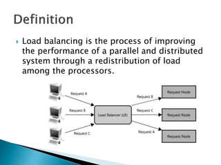
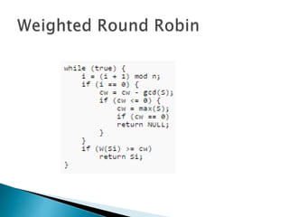
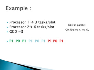
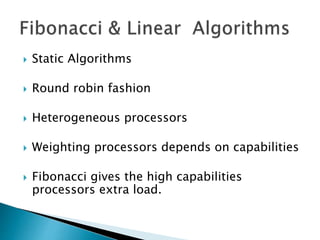
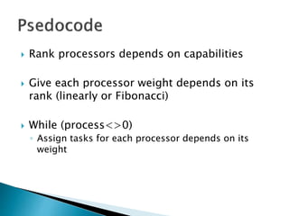
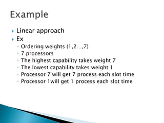
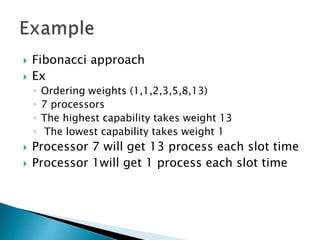
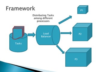
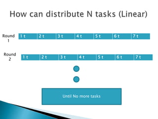
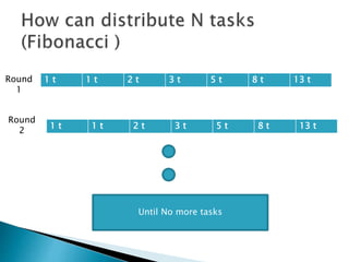
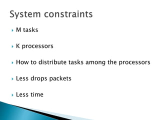
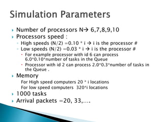
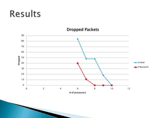
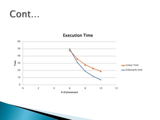
Omar Darwish
 Load balancing is the process of improving
the performance of a parallel and distributed
system through a redistribution of load
among the processors.
Who Initialized the load balancing algorithm ?
 Sender Initiated
◦ Initialized by the sender.
◦ Sender sends request messages till it finds a
receiver that can accept the load.
 Receiver Initiated
◦ Initiated by the receiver.
◦ Receiver sends request messages till it finds a
sender that can get the load.
 The performance of the processors is
determined at the beginning of execution.
 Master processor and slave processors.
 A task is always executed on the processor to
which it is assigned.
 Reduce the execution time, minimizing the
communication delays
 Round Robin Algorithm
◦ Processor choosing is performed in series and will
be back to the first processor if the last processor
has been reached.
 Randomized Algorithm
◦ Uses random numbers to choose slave processors
based on statistics .
 Central Manager Algorithm
◦ The central processor is able to gather all slave
processors load information
◦ The chosen slave processor is the processor having
the least load
 Threshold Algorithm
◦ The processes are assigned immediately upon
creation to hosts.
◦ Under loaded, medium and overloaded.
 Dynamic algorithms allocate processes
dynamically when one of the processors
becomes under loaded.
 Buffered in the queue
 Allocated dynamically upon requests from
remote hosts
 Central Queue
◦ Stores new activities and unfulfilled requests as a
cyclic FIFO queue on the main host.
 Local Queue
 A parameter defines the minimal number of
ready processes the load manager attempts
to provide on each processor
 Adaptability
◦ Static No, Dynamic Yes
 Predictability
◦ Static Yes, Dynamic No
 Waiting Time (Queuing time )
 Execution System
 Fitness Function
◦ The main objective of GA is to find a schedule with
optimal cost while load-balancing.
 Less execution time.
 Less communication cost.
 Higher processor utilization.
 Maximum system throughput
 Selection
 Processors permutation
 Crossover
 Exchange portions between strings.
 Mutation
 Change the genes in a chromosome
(Processors set)
 NP complete problem.
 Untractable with large N of tasks and P
number of processors.
Actual execution cost
If we consider communication time, the work
load L is
 Objective function
 Processor 1  3 tasks/slot
 Processor 2 6 tasks/slot
 GCD =3
 P1 P0 P1 P1 P0 P1 P1 P0 P1
O(n log log n/log n),
GCD in parallel
 Static Algorithms
 Round robin fashion
 Heterogeneous processors
 Weighting processors depends on capabilities
 Fibonacci gives the high capabilities
processors extra load.
 Rank processors depends on capabilities
 Give each processor weight depends on its
rank (linearly or Fibonacci)
 While (process<>0)
◦ Assign tasks for each processor depends on its
weight
 Linear approach
 Ex
◦ Ordering weights (1,2…,7)
◦ 7 processors
◦ The highest capability takes weight 7
◦ The lowest capability takes weight 1
◦ Processor 7 will get 7 process each slot time
◦ Processor 1will get 1 process each slot time
 Fibonacci approach
 Ex
◦ Ordering weights (1,1,2,3,5,8,13)
◦ 7 processors
◦ The highest capability takes weight 13
◦ The lowest capability takes weight 1
 Processor 7 will get 13 process each slot time
 Processor 1will get 1 process each slot time
Load
Balancer
Tasks
P1
P2
P3
Distributing Tasks
among different
processors
1 t 2 t 3 t 4 t 5 t 6 t 7 t
Round
1
1 t 2 t 3 t 4 t 5 t 6 t 7 t
Round
2
Until No more tasks
1 t 1 t 2 t 3 t 5 t 8 t 13 t
Round
1
1 t 1 t 2 t 3 t 5 t 8 t 13 t
Round
2
Until No more tasks
 M tasks
 K processors
 How to distribute tasks among the processors
 Less drops packets
 Less time
 Number of processors N 6,7,8,9,10
 Processors speed :
◦ High speeds (N/2) =0.10 * i  i is the processor #
◦ Low speeds (N/2) =0.03 * i  i is the processor #
 For example processor with id 6 can process
6.0*0.10*number of tasks in the Queue
 Processor with id 2 can process 2.0*0.3*number of tasks in
the Queue .
 Memory
For High speed computers 20 * i locations
For low speed computers 320*i locations
 1000 tasks
 Arrival packets =20, 33,….
0
10
20
30
40
50
60
70
80
90
0 2 4 6 8 10 12
Dropped
# of processors
Dropped Packets
Linear
Fibonachi
0
10
20
30
40
50
60
0 2 4 6 8 10 12
Time
# of processors
Execution Time
Linear Time
Febonachi time
 Fibonacci distribution guarantee the more
utilization of higher capabilities processors
and less load on the less capabilities
processors.
 The presentation explore:
◦ Static vs. Dynamic load balancing technique.
◦ The formulization of task scheduling problem.
 Sharma, Sandeep, Sarabjit Singh, and Meenakshi Sharma. "Performance analysis of
load balancing algorithms." World Academy of Science, Engineering and
Technology 38 (2008): 269-272.
 Rajguru, Abhijit A., and S. S. Apte. "A Comparative Performance Analysis of Load
Balancing Algorithms in Distributed System using Qualitative
Parameters." International Journal of Recent Technology and Engineering 1.3
(2012).
 Shah, Purnima, and S. M. Shah. "Load Balancing in Distributed System Using
Genetic Algorithm}." Special issues on IP Multimedia Communications}: 139-142.
 Attiya, Gamal, and Yskandar Hamam. "Task allocation for minimizing programs
completion time in multicomputer systems." Computational Science and Its
Applications–ICCSA 2004. Springer Berlin Heidelberg, 2004. 97-106.
 Chor, Benny, and Oded Goldreich. "An improved parallel algorithm for integer
GCD." Algorithmica 5.1-4 (1990): 1-10.
 http://kb.linuxvirtualserver.org/wiki/Weighted_Round-Robin_Scheduling
Questions ?

LoadBalancing .pptx

  • 1.
  • 2.
     Load balancingis the process of improving the performance of a parallel and distributed system through a redistribution of load among the processors.
  • 3.
    Who Initialized theload balancing algorithm ?  Sender Initiated ◦ Initialized by the sender. ◦ Sender sends request messages till it finds a receiver that can accept the load.  Receiver Initiated ◦ Initiated by the receiver. ◦ Receiver sends request messages till it finds a sender that can get the load.
  • 4.
     The performanceof the processors is determined at the beginning of execution.  Master processor and slave processors.  A task is always executed on the processor to which it is assigned.  Reduce the execution time, minimizing the communication delays
  • 5.
     Round RobinAlgorithm ◦ Processor choosing is performed in series and will be back to the first processor if the last processor has been reached.  Randomized Algorithm ◦ Uses random numbers to choose slave processors based on statistics .
  • 6.
     Central ManagerAlgorithm ◦ The central processor is able to gather all slave processors load information ◦ The chosen slave processor is the processor having the least load  Threshold Algorithm ◦ The processes are assigned immediately upon creation to hosts. ◦ Under loaded, medium and overloaded.
  • 7.
     Dynamic algorithmsallocate processes dynamically when one of the processors becomes under loaded.  Buffered in the queue  Allocated dynamically upon requests from remote hosts
  • 8.
     Central Queue ◦Stores new activities and unfulfilled requests as a cyclic FIFO queue on the main host.  Local Queue  A parameter defines the minimal number of ready processes the load manager attempts to provide on each processor
  • 9.
     Adaptability ◦ StaticNo, Dynamic Yes  Predictability ◦ Static Yes, Dynamic No  Waiting Time (Queuing time )  Execution System
  • 10.
     Fitness Function ◦The main objective of GA is to find a schedule with optimal cost while load-balancing.  Less execution time.  Less communication cost.  Higher processor utilization.  Maximum system throughput
  • 11.
     Selection  Processorspermutation  Crossover  Exchange portions between strings.  Mutation  Change the genes in a chromosome (Processors set)
  • 12.
     NP completeproblem.  Untractable with large N of tasks and P number of processors.
  • 13.
    Actual execution cost Ifwe consider communication time, the work load L is
  • 14.
  • 16.
     Processor 1 3 tasks/slot  Processor 2 6 tasks/slot  GCD =3  P1 P0 P1 P1 P0 P1 P1 P0 P1 O(n log log n/log n), GCD in parallel
  • 17.
     Static Algorithms Round robin fashion  Heterogeneous processors  Weighting processors depends on capabilities  Fibonacci gives the high capabilities processors extra load.
  • 18.
     Rank processorsdepends on capabilities  Give each processor weight depends on its rank (linearly or Fibonacci)  While (process<>0) ◦ Assign tasks for each processor depends on its weight
  • 19.
     Linear approach Ex ◦ Ordering weights (1,2…,7) ◦ 7 processors ◦ The highest capability takes weight 7 ◦ The lowest capability takes weight 1 ◦ Processor 7 will get 7 process each slot time ◦ Processor 1will get 1 process each slot time
  • 20.
     Fibonacci approach Ex ◦ Ordering weights (1,1,2,3,5,8,13) ◦ 7 processors ◦ The highest capability takes weight 13 ◦ The lowest capability takes weight 1  Processor 7 will get 13 process each slot time  Processor 1will get 1 process each slot time
  • 21.
  • 22.
    1 t 2t 3 t 4 t 5 t 6 t 7 t Round 1 1 t 2 t 3 t 4 t 5 t 6 t 7 t Round 2 Until No more tasks
  • 23.
    1 t 1t 2 t 3 t 5 t 8 t 13 t Round 1 1 t 1 t 2 t 3 t 5 t 8 t 13 t Round 2 Until No more tasks
  • 24.
     M tasks K processors  How to distribute tasks among the processors  Less drops packets  Less time
  • 25.
     Number ofprocessors N 6,7,8,9,10  Processors speed : ◦ High speeds (N/2) =0.10 * i  i is the processor # ◦ Low speeds (N/2) =0.03 * i  i is the processor #  For example processor with id 6 can process 6.0*0.10*number of tasks in the Queue  Processor with id 2 can process 2.0*0.3*number of tasks in the Queue .  Memory For High speed computers 20 * i locations For low speed computers 320*i locations  1000 tasks  Arrival packets =20, 33,….
  • 26.
    0 10 20 30 40 50 60 70 80 90 0 2 46 8 10 12 Dropped # of processors Dropped Packets Linear Fibonachi
  • 27.
    0 10 20 30 40 50 60 0 2 46 8 10 12 Time # of processors Execution Time Linear Time Febonachi time
  • 28.
     Fibonacci distributionguarantee the more utilization of higher capabilities processors and less load on the less capabilities processors.
  • 29.
     The presentationexplore: ◦ Static vs. Dynamic load balancing technique. ◦ The formulization of task scheduling problem.
  • 30.
     Sharma, Sandeep,Sarabjit Singh, and Meenakshi Sharma. "Performance analysis of load balancing algorithms." World Academy of Science, Engineering and Technology 38 (2008): 269-272.  Rajguru, Abhijit A., and S. S. Apte. "A Comparative Performance Analysis of Load Balancing Algorithms in Distributed System using Qualitative Parameters." International Journal of Recent Technology and Engineering 1.3 (2012).  Shah, Purnima, and S. M. Shah. "Load Balancing in Distributed System Using Genetic Algorithm}." Special issues on IP Multimedia Communications}: 139-142.  Attiya, Gamal, and Yskandar Hamam. "Task allocation for minimizing programs completion time in multicomputer systems." Computational Science and Its Applications–ICCSA 2004. Springer Berlin Heidelberg, 2004. 97-106.  Chor, Benny, and Oded Goldreich. "An improved parallel algorithm for integer GCD." Algorithmica 5.1-4 (1990): 1-10.  http://kb.linuxvirtualserver.org/wiki/Weighted_Round-Robin_Scheduling
  • 31.