Deterministic Inventory Models. Waiting Line Model. Operations research portion for M.SC Maths.

1. INVENTORY/PRODUCTION
MANAGEMENT - I
(Deterministic Inventory Models)

2. Inventory and Inventory Decisions
Inventory may be defined as the stock of
goods, commodities or other
economic resources that are stored
or reserved in order to ensure
smooth and efficient running of
business affairs.
The term inventory maybe classified in
two main categories:
 Direct Inventory : The items which
play a direct role in manufacture
and become an integral part of
finished goods are included in this
category such as (i) Raw materials,
(ii) Work in process goods, (iii)
Finished goods, and (iv) Spare
parts.
 Indirect Inventory : The items
which are necessarily required for
manufacturing but do not become
the component of finished
production like: oil, grease,
lubricants, petrol, office material,
maintenance material, etc.

3. COSTS INVOLVED INVENTORY
PROBLEMS
 Holding cost : The cost associated with carrying or holding the goods in stock is
known as holding or carrying cost which is usually denoted by C1 or Ch per unit of
goods for a unit of time. This cost is assumed to vary directly with the size of
inventory as well as the time for which the item is held in stock.
 Shortage cost : The penalty costs that are incurred as a result of running out of stock
(i.e. shortage) are known as shortage or stock-out costs. These are denoted by C2 or
Cs per unit of goods for a specified period.
 Set-up cost : These include the fixed costs associated with obtaining goods through
placing of an order or purchasing or manufacturing or setting up a machinery before
starting production. So they include costs of purchase, requisition, follow-up,
receiving the goods, quality control, etc. These are also called order costs or
replenishment costs, usually denoted by C3 or Co per production run (cycle). They
are assumed to be independent of the quantity ordered or produced.

4. LIMITATIONS OF EOQ FORMULAE
1. The demand is neither known with certainty nor it is uniform in practical situation.
2. It is difficult to measure the ordering cost and also it is not linearly related to the
number of orders and rises in stepped manner with the increasing number of orders.
3. In EOQ models, it is assumed that the annual demand can be estimated in advance.
But, annual demand can not be simply estimated with accuracy.
4. In EOQ model, it assumed that the inventory rises to its maximum level
instantaneously. But, in many cases it may not be true because the orders may be
delivered in portions over a period of time
5. In EOQ, it is assumed that the demand is uniform. But, uniformity is seldom
observed in practical situations.
6. In EOQ models, the replenishment time is assumed to be zero. But, this is not
possible unless the supplier is nearby.
7. If the EOQ models are applied without due regard to the possibility of a falling
demand, the it can lead to a high value of obsolenscence inventory.

5. THE EOQ MODEL WITHOUT SHORTAGE
Model I (a) : The Economic Lot Size System with Uniform Demand
Assumptions :
1) Demand is uniform at the rate of R quantity units per unit time.
2) Lead time is zero (or known exactly).
3) Production rate is infinite, i.e. production is instantaneous.
4) Shortages are not allowed.
5) Holding cost is rupees C1 per quantity per unit time.
6) Set-up cost is rupees C3 per set-up.
Derivation:
Average inventory = ½ [maximum level + minimum level] = ½ [ q + 0] = q/2.
Total inventory carrying cost per unit =average no. of units in inventory X cost of one unit X inventory carrying cost percentage
= ½ qCI = ½ qC1
Cost Equation
Total inventory costs = Total inventory carrying cost + total annual ordering costs
C(q) = ½ qC1 + (R/q) C3
Optimal EOQ
½ qC1 = (R/q) C3 => qC1 = (2R/q) C3 => q2 = 2RC3/ C1
 q= (2C3R/C1)
 Optimal q* (EOQ) = (2 X set-up cost X demand rate / carrying cost)

6. Optimum inventory cost
Cmin = (2C1C3R)
Optimum inventory cost Cmin = (2 X carrying cost X set-up cost X demand rate )
Optimum ordering interval
EOQ= demand rate X interval of ordering
=> q = R X t
 t = q/ R = (2C3/RC1)
 Optimum ordering interval t* = (2 X set-up cost X / demand rate X carrying cost)
Optimum number of orders
N= R/ q
=> Optimum number of orders = demand rate / EOQ
Number of days supply d = 365/ N = 365/ Optimum number of orders
Model I (b) : The Economic Lot Size System with different rates of demand in different cycles
Assumption : The rate of demand D differs with different production cycles.
Derivation :
Let the total demand D be specified as demand during total time period T and q be the stock level to be fixed.
Ordering cost = Number of orders X C3 = (D/ q) C3
Carrying cost = Average inventory X C1 X T = (q/ 2) C1T
Cost Equation
C(q) = (q/ 2) C1T + (D/ q) C3

7. Optimal EOQ
(q/ 2) C1T = (D/ q) C3 => q2 = 2DC3/ C1T
q= (2C3D/C1T)
 Optimal q* (EOQ) = (2 X set-up cost X demand rate / carrying cost X time period)
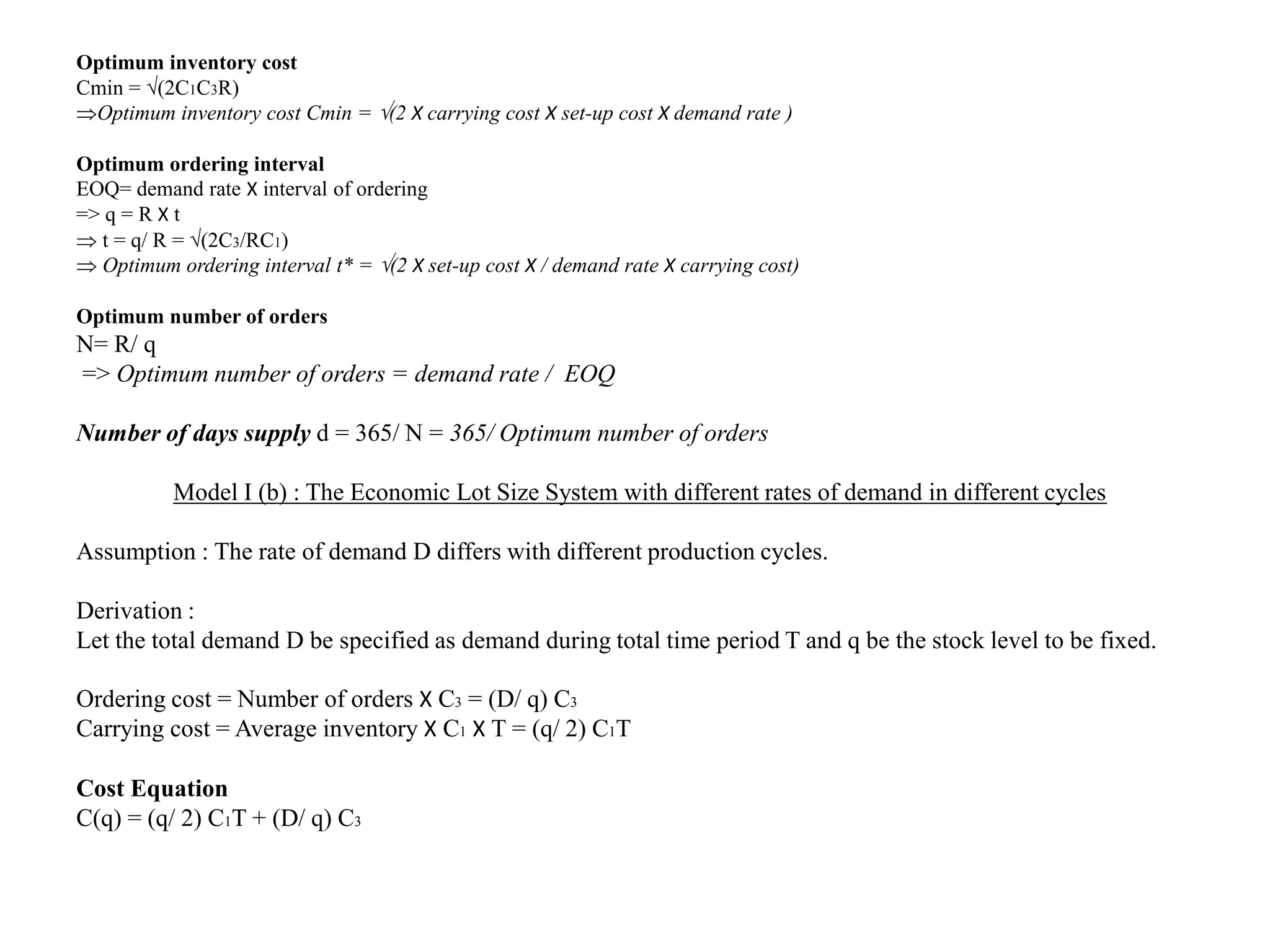
Optimum inventory cost
Cmin = (2C1C3D/ T)
Optimum inventory cost Cmin = (2 X carrying cost X set-up cost X demand rate / time period)
Model I (c) : The Economic Lot Size System with different rates of demand in different cycles
Assumptions :
C2 = infinity, R= no. Of items required per unit time, K= no. Of items produced per unit time, t= interval between production
cycles.
Derivation :
Ordering cost = Number of orders X C3 = (R/ q) C3
Carrying cost = Average inventory X C1 X T = ½ [q/ K] (K - R) C1
Cost Equation
C(q) = ½ [q/ K] (K – R) C1 + (R/ q) C3
Optimal EOQ
½ [q/ K] (K - R )C1 = (R/ q) C3 => q2 = 2RC3/ C1(1- R/ K)
 q*= (2RC3/C1(1 – R/ K))
Optimum time interval
t*= (2C3/C1R(1 – R/ K))
Optimum inventory cost
Cmin = (2C1C3R ( 1- R/ K))

8. THE EOQ MODEL WHEN SHORTAGES ARE ALLOWED
Model II (a) : The Economic Lot Size System with Constant rate of Demand, Scheduling Time Constant
Assumptions :
1) C1 is the holding cost per quantity per unit time.
2) C2 is the holding cost per quantity per unit time.
3) R quantity per unit time is the demand rate.
4) Production rate is infinite.
5) tp is the scheduling time period which is constant.
6) qp is the fixed lot size.
7) z is the order level to which the inventory is raised in the beginning of each scheduling period.
8) Lead time is zero.
Derivation:
Holding cost= ½ (z2 C1/ qp)
Shortage cost = ½ (C2 / qp) (qp – z ) 2
Cost Equation
C(z) = ½ (z2 C1/ qp) + ½ (C2 / qp) (qp – z ) 2
Optimal EOQ
(dC/ dz )=0 => z= (C2/ C1 + C2) qp
 z= (C2/ C1 + C2) Rtp
Optimum inventory cost
Cmin = (C1C2/ 2(C1 + C2)) Rtp

9. Model II (b) : The EOQ with Constant rate of Demand, Scheduling Time Variable
Assumptions :
1) t is the scheduling time period which is variable.
2) q = Rt is the order quantity per run.
Derivation :
Cost Equation C(t, z) = 1/t [ (C1z2 / 2R) + ½ (C2 / R) ( Rt – z )2 + C3 ]
Reorder time t= (2C3 (C1 + C2) / RC1C2)
Optimal EOQ q*= Rt* = (2RC3 (C1 + C2) / C1C2)
Optimum inventory cost Cmin = (2C1C3R (C2 / (C1 + C2) )
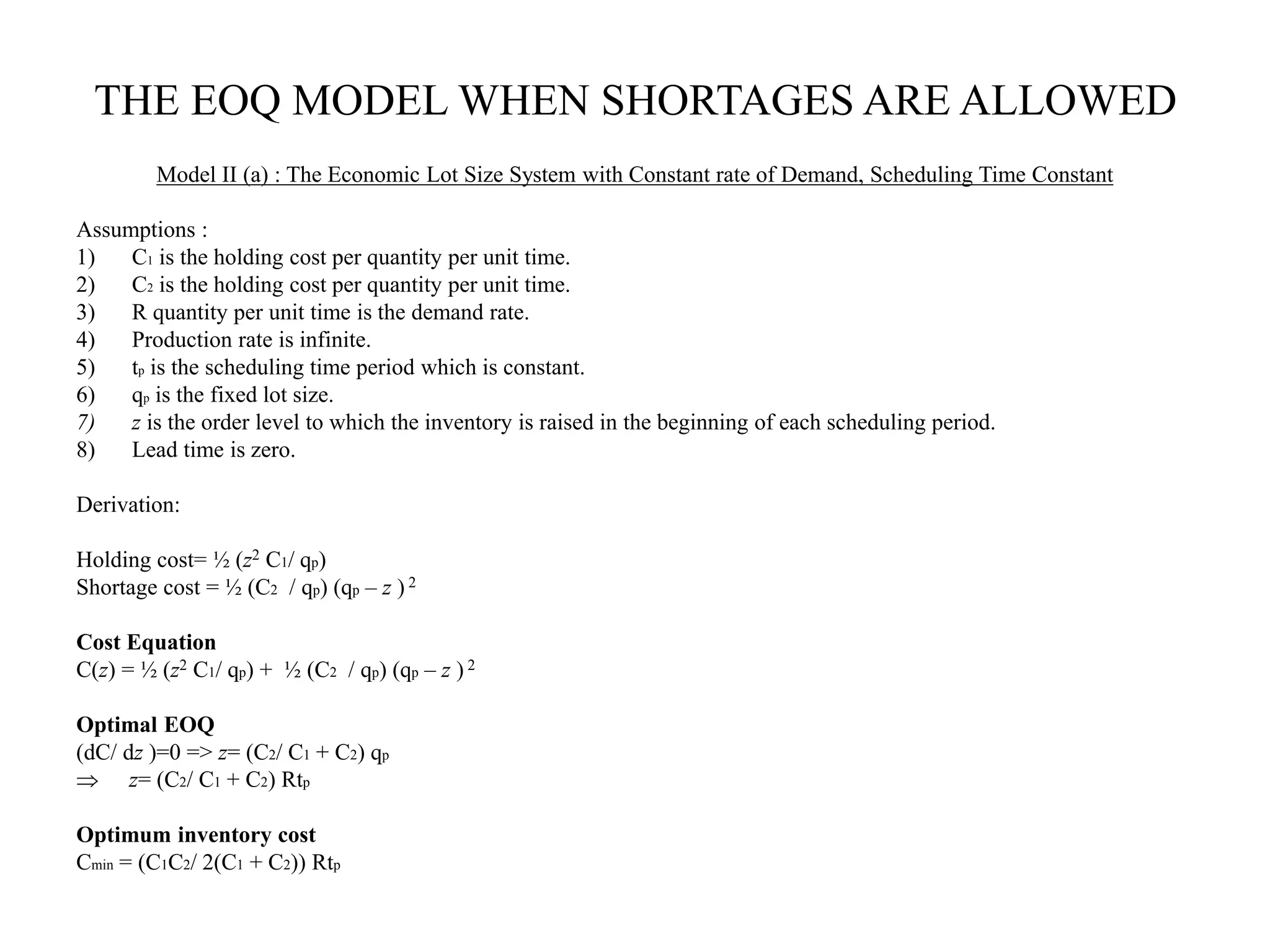
Model II (c) : The Production Lot Size with Shortages
Assumptions :
1) R units per unit time is the uniform demand rate.
2) Production rate K units per unit time is finite, K > R.
3) Shortages are allowed and backlogged.
Derivation :
Cost Equation C(t2, t3) = ½ [ (C1t22 + C2t32 ) RK + ½ (C2 / R) ( Rt – z )2 + C3 ]
Optimal EOQ q*= (2RC3 (C1 + C2) / C1C2) (1/ (1 – R/ K)) = (2RC1C3 (1-R/ K) / (C1 + C2) C2)
Optimum inventory cost Cmin = (2RC1 C2 C3 (1-R / K) / (C1 + C2) )

10. QUEUEING THEORY
(Waiting Line Model)

11. Queueing System
 A queue is a line or sequence of
people or vehicles awaiting their turn
to be attended or to proceed.
 Queueing systems are simplified
mathematical model to explain
congestion.
 A queueing system can be completely
described by:
a) the input ( or arrival pattern ) ,
b) the service mechanism ( or service
pattern ) ,
c) the queue discipline , and
d) customer’s behavior .

12. Customer’s Behaviour and System’s Behaviour
The customers generally behave in four ways:
1. Balking : A customer may leave the queue because the queue is too long and has no
time to wait , or there is no sufficient waiting space.
2. Reneging : This happens when a waiting customer leaves the queue due to
impatience.
3. Priorities : In certain applications, some customers are served before others
regardless of their order of arrival. These customers have priority over others.
4. Jockeying : Customers may jockey from one waiting line to another. It may be seen
that this happens in a supermarket.
The system behaviour changes over time . These changes are broadly classified into
two states :
 A system is said to be in transient state when its operating characteristics are
dependent on time.
 A steady state condition is said to prevail when the behaviour of the system
becomes independent of time.

13. List of Symbols
 n = number of units in the system.
 Pn (t) = transient state probability that exactly n calling units are in the queueing system at
time t.
 Pn = steady state probability of having n units in the system.
 n = mean arrival rate of customers when n units are present in the system.
 n = mean service rate when n units are present in the system.
  = mean arrival rate of customers when n is constant for all n.
  = mean arrival rate of customers when n is constant for all n.
 s = number of parallel service stations.
  =  /  s = traffic intensity for servers facility, i.e., the expected fraction of time the servers
are busy.
 Ls = expected line length, i.e., expected number of customers in the system.
 Lq = expected queue length, i.e., expected number of customers in the queue.
 Ws = expected waiting time per customer in the system.
 Wq = expected waiting time per customer in the system.
 ( W W > 0 ) = expected waiting time of a customer who has to wait.
 ( L L > 0 ) = expected length of non-empty queues.
 P ( W > 0 ) = probability of customer having to wait for service.

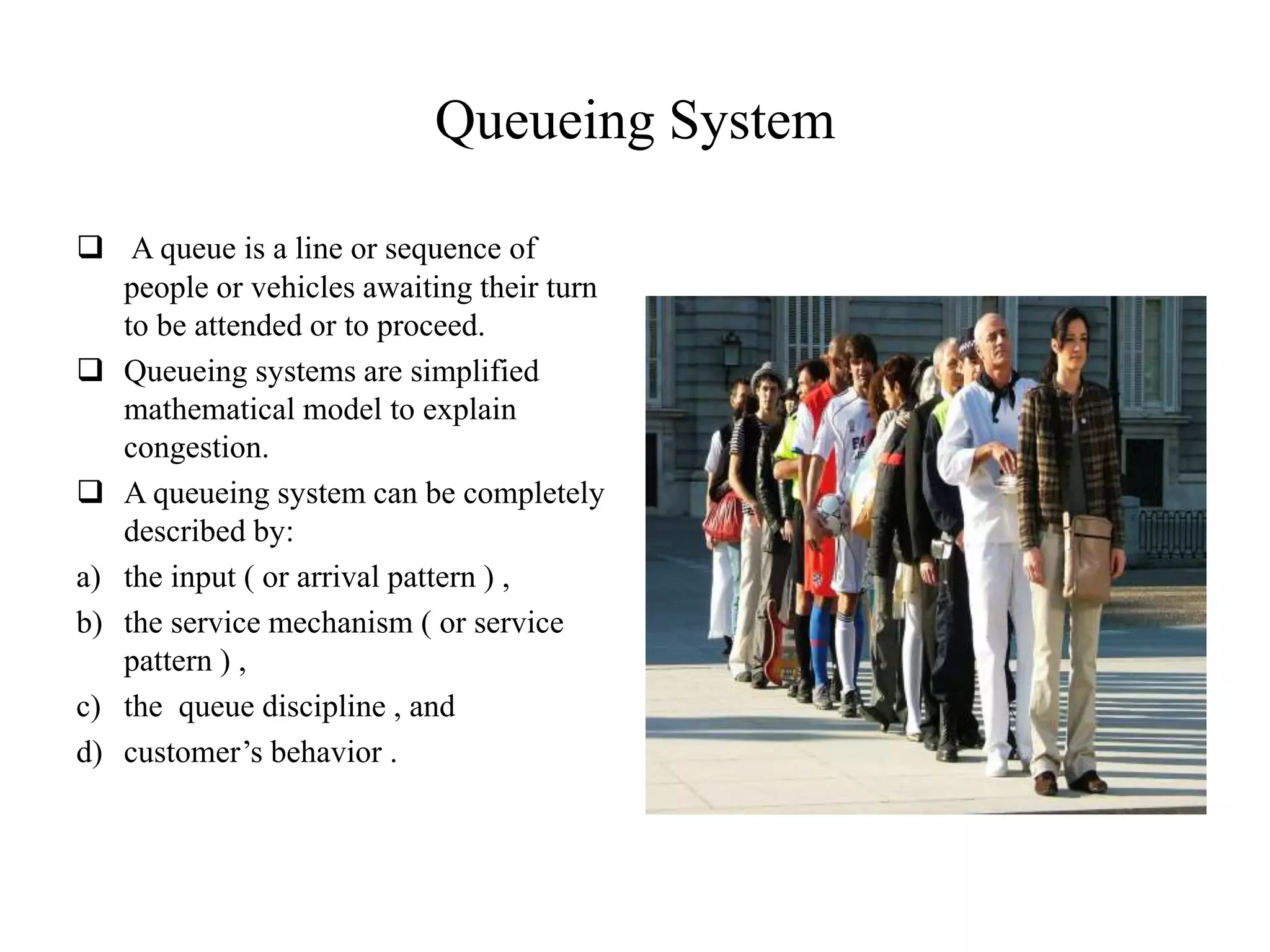
14. Model IV (A) : (M|M|S) : (|FCFS )
The overall service rate when there are n units in the system may be obtained in the following two situations :
i. If n ≤ s, all the customers may be served simultaneously. There will be no queue, ( s – n ) number of servers
may remain idle, and then n = n, n = 0, 1, 2, …. , s.
ii. If n ≥ s, all the servers are busy, maximum number of customers waiting in the queue will be ( n – s ), then
n = s.
To obtain the system of steady state equations:
0 = -P0 + P1 for n = 0 ….. (1)
0 = - (  + n ) Pn +  Pn-1 + ( n+1 )  Pn+1 for 0<n<s ….(2)
0 = - (  + s ) Pn +  Pn-1 + s Pn+1 for n > s ……(3)
To solve the system of difference equations (1) , (2) , and (3) :
P0 = P0 [initially],
P1 = ( / ) P0 [from (1)],
P2 = ( / 2) P1 = ( 2 / 2! 2 ) P1 [from (2)],
P3 = ( / 3) P1 = ( 3 / 3! 3 ) P2 [from (2)],
………………………………………………..
In general, Pn = ( / n) Pn-1 = ( n / n! n ) Pn-1 { for 1 ≤ n ≤ s } [from (2)].
...............................................................................
Ps = (1/ s!) (  /  )s P0
Ps+1 = (1/ s) (1/ s!) (  /  )s+1 P0
Ps+2 = (1/ s2) (1/ s!) (  /  )s+2 P0
In general, Pn = (1/ sn-s) (1/ s!) (  /  )n P0 , [ for n ≥ s ].

15. We know that, Ss-1
n=0 (Pn) + S 
n=s (Pn)
P0 = S s-1
n=0 ((s)n / n!) + ( ss / s! ) (s / 1 - )
Measures :
Lq = S
n=s (n – s) Pn = Ps (  / (1 - )2 )
Ls = Lq + s + Ss-1
n=0 [(n – s) (s)n P0 / n!]
Wq = Lq /  = Ps ( 1 / s(1 - )2 )
Ws = Ls /  = Wq + 1 / 
( L | L > 0) = [ S
n=s+1 (n – s) Pn S
n=s+1 Pn ] = 1 / (1 - )
( W | W > 0) = 1 / (s - )