This document provides an overview of Linux performance and tuning guidelines. It discusses Linux processes, memory, file systems, I/O subsystems, networking, and performance monitoring tools. The document is intended to help readers understand how Linux works and how to optimize system performance.

1. ibm.com/redbooks Redpaper
Front cover
Linux Performance and
Tuning Guidelines
Eduardo Ciliendo
Takechika Kunimasa
Operating system tuning methods
Performance monitoring tools
Performance analysis
Click here to check for updates

3. International Technical Support Organization
Linux Performance and Tuning Guidelines
July 2007
REDP-4285-00

4. © Copyright International Business Machines Corporation 2007. All rights reserved.
Note to U.S. Government Users Restricted Rights -- Use, duplication or disclosure restricted by GSA ADP Schedule
Contract with IBM Corp.
First Edition (July 2007)
This edition applies to kernel 2.6 Linux distributions.
This paper was updated on April 25, 2008.
Note: Before using this information and the product it supports, read the information in “Notices” on
page vii.

5. © Copyright IBM Corp. 2007. All rights reserved. iii
Contents
Notices . . . . . . . . . . . . . . . . . . . . . . . . . . . . . . . . . . . . . . . . . . . . . . . . . . . . . . . . . . . . . . . . . vii
Trademarks . . . . . . . . . . . . . . . . . . . . . . . . . . . . . . . . . . . . . . . . . . . . . . . . . . . . . . . . . . . . . viii
Preface . . . . . . . . . . . . . . . . . . . . . . . . . . . . . . . . . . . . . . . . . . . . . . . . . . . . . . . . . . . . . . . . . ix
How this paper is structured. . . . . . . . . . . . . . . . . . . . . . . . . . . . . . . . . . . . . . . . . . . . . . . . . . ix
The team that wrote this paper . . . . . . . . . . . . . . . . . . . . . . . . . . . . . . . . . . . . . . . . . . . . . . . .x
Become a published author . . . . . . . . . . . . . . . . . . . . . . . . . . . . . . . . . . . . . . . . . . . . . . . . . . xi
Comments welcome. . . . . . . . . . . . . . . . . . . . . . . . . . . . . . . . . . . . . . . . . . . . . . . . . . . . . . . . xii
Chapter 1. Understanding the Linux operating system. . . . . . . . . . . . . . . . . . . . . . . . . . 1
1.1 Linux process management . . . . . . . . . . . . . . . . . . . . . . . . . . . . . . . . . . . . . . . . . . . . . . 2
1.1.1 What is a process? . . . . . . . . . . . . . . . . . . . . . . . . . . . . . . . . . . . . . . . . . . . . . . . . . 2
1.1.2 Life cycle of a process . . . . . . . . . . . . . . . . . . . . . . . . . . . . . . . . . . . . . . . . . . . . . . 3
1.1.3 Thread. . . . . . . . . . . . . . . . . . . . . . . . . . . . . . . . . . . . . . . . . . . . . . . . . . . . . . . . . . . 4
1.1.4 Process priority and nice level . . . . . . . . . . . . . . . . . . . . . . . . . . . . . . . . . . . . . . . . 5
1.1.5 Context switching . . . . . . . . . . . . . . . . . . . . . . . . . . . . . . . . . . . . . . . . . . . . . . . . . . 5
1.1.6 Interrupt handling . . . . . . . . . . . . . . . . . . . . . . . . . . . . . . . . . . . . . . . . . . . . . . . . . . 6
1.1.7 Process state . . . . . . . . . . . . . . . . . . . . . . . . . . . . . . . . . . . . . . . . . . . . . . . . . . . . . 6
1.1.8 Process memory segments. . . . . . . . . . . . . . . . . . . . . . . . . . . . . . . . . . . . . . . . . . . 8
1.1.9 Linux CPU scheduler . . . . . . . . . . . . . . . . . . . . . . . . . . . . . . . . . . . . . . . . . . . . . . . 9
1.2 Linux memory architecture . . . . . . . . . . . . . . . . . . . . . . . . . . . . . . . . . . . . . . . . . . . . . . 10
1.2.1 Physical and virtual memory . . . . . . . . . . . . . . . . . . . . . . . . . . . . . . . . . . . . . . . . . 10
1.2.2 Virtual memory manager. . . . . . . . . . . . . . . . . . . . . . . . . . . . . . . . . . . . . . . . . . . . 12
1.3 Linux file systems . . . . . . . . . . . . . . . . . . . . . . . . . . . . . . . . . . . . . . . . . . . . . . . . . . . . . 15
1.3.1 Virtual file system . . . . . . . . . . . . . . . . . . . . . . . . . . . . . . . . . . . . . . . . . . . . . . . . . 15
1.3.2 Journaling . . . . . . . . . . . . . . . . . . . . . . . . . . . . . . . . . . . . . . . . . . . . . . . . . . . . . . . 16
1.3.3 Ext2. . . . . . . . . . . . . . . . . . . . . . . . . . . . . . . . . . . . . . . . . . . . . . . . . . . . . . . . . . . . 17
1.3.4 Ext3. . . . . . . . . . . . . . . . . . . . . . . . . . . . . . . . . . . . . . . . . . . . . . . . . . . . . . . . . . . . 18
1.3.5 ReiserFS . . . . . . . . . . . . . . . . . . . . . . . . . . . . . . . . . . . . . . . . . . . . . . . . . . . . . . . . 19
1.3.6 Journal File System . . . . . . . . . . . . . . . . . . . . . . . . . . . . . . . . . . . . . . . . . . . . . . . 19
1.3.7 XFS . . . . . . . . . . . . . . . . . . . . . . . . . . . . . . . . . . . . . . . . . . . . . . . . . . . . . . . . . . . . 19
1.4 Disk I/O subsystem . . . . . . . . . . . . . . . . . . . . . . . . . . . . . . . . . . . . . . . . . . . . . . . . . . . . 19
1.4.1 I/O subsystem architecture . . . . . . . . . . . . . . . . . . . . . . . . . . . . . . . . . . . . . . . . . . 20
1.4.2 Cache . . . . . . . . . . . . . . . . . . . . . . . . . . . . . . . . . . . . . . . . . . . . . . . . . . . . . . . . . . 21
1.4.3 Block layer . . . . . . . . . . . . . . . . . . . . . . . . . . . . . . . . . . . . . . . . . . . . . . . . . . . . . . 23
1.4.4 I/O device driver . . . . . . . . . . . . . . . . . . . . . . . . . . . . . . . . . . . . . . . . . . . . . . . . . . 24
1.4.5 RAID and storage system . . . . . . . . . . . . . . . . . . . . . . . . . . . . . . . . . . . . . . . . . . . 25
1.5 Network subsystem. . . . . . . . . . . . . . . . . . . . . . . . . . . . . . . . . . . . . . . . . . . . . . . . . . . . 26
1.5.1 Networking implementation. . . . . . . . . . . . . . . . . . . . . . . . . . . . . . . . . . . . . . . . . . 26
1.5.2 TCP/IP . . . . . . . . . . . . . . . . . . . . . . . . . . . . . . . . . . . . . . . . . . . . . . . . . . . . . . . . . 30
1.5.3 Offload . . . . . . . . . . . . . . . . . . . . . . . . . . . . . . . . . . . . . . . . . . . . . . . . . . . . . . . . . 33
1.5.4 Bonding module . . . . . . . . . . . . . . . . . . . . . . . . . . . . . . . . . . . . . . . . . . . . . . . . . . 34
1.6 Understanding Linux performance metrics . . . . . . . . . . . . . . . . . . . . . . . . . . . . . . . . . . 34
1.6.1 Processor metrics . . . . . . . . . . . . . . . . . . . . . . . . . . . . . . . . . . . . . . . . . . . . . . . . . 34
1.6.2 Memory metrics. . . . . . . . . . . . . . . . . . . . . . . . . . . . . . . . . . . . . . . . . . . . . . . . . . . 35
1.6.3 Network interface metrics . . . . . . . . . . . . . . . . . . . . . . . . . . . . . . . . . . . . . . . . . . . 36
1.6.4 Block device metrics . . . . . . . . . . . . . . . . . . . . . . . . . . . . . . . . . . . . . . . . . . . . . . . 36
Chapter 2. Monitoring and benchmark tools . . . . . . . . . . . . . . . . . . . . . . . . . . . . . . . . . 39

6. iv Linux Performance and Tuning Guidelines
2.1 Introduction . . . . . . . . . . . . . . . . . . . . . . . . . . . . . . . . . . . . . . . . . . . . . . . . . . . . . . . . . . 40
2.2 Overview of tool functions . . . . . . . . . . . . . . . . . . . . . . . . . . . . . . . . . . . . . . . . . . . . . . . 40
2.3 Monitoring tools. . . . . . . . . . . . . . . . . . . . . . . . . . . . . . . . . . . . . . . . . . . . . . . . . . . . . . . 41
2.3.1 top . . . . . . . . . . . . . . . . . . . . . . . . . . . . . . . . . . . . . . . . . . . . . . . . . . . . . . . . . . . . . 41
2.3.2 vmstat . . . . . . . . . . . . . . . . . . . . . . . . . . . . . . . . . . . . . . . . . . . . . . . . . . . . . . . . . . 42
2.3.3 uptime . . . . . . . . . . . . . . . . . . . . . . . . . . . . . . . . . . . . . . . . . . . . . . . . . . . . . . . . . . 43
2.3.4 ps and pstree . . . . . . . . . . . . . . . . . . . . . . . . . . . . . . . . . . . . . . . . . . . . . . . . . . . . 44
2.3.5 free . . . . . . . . . . . . . . . . . . . . . . . . . . . . . . . . . . . . . . . . . . . . . . . . . . . . . . . . . . . . 46
2.3.6 iostat . . . . . . . . . . . . . . . . . . . . . . . . . . . . . . . . . . . . . . . . . . . . . . . . . . . . . . . . . . . 48
2.3.7 sar . . . . . . . . . . . . . . . . . . . . . . . . . . . . . . . . . . . . . . . . . . . . . . . . . . . . . . . . . . . . . 50
2.3.8 mpstat . . . . . . . . . . . . . . . . . . . . . . . . . . . . . . . . . . . . . . . . . . . . . . . . . . . . . . . . . . 51
2.3.9 numastat . . . . . . . . . . . . . . . . . . . . . . . . . . . . . . . . . . . . . . . . . . . . . . . . . . . . . . . . 52
2.3.10 pmap . . . . . . . . . . . . . . . . . . . . . . . . . . . . . . . . . . . . . . . . . . . . . . . . . . . . . . . . . . 52
2.3.11 netstat . . . . . . . . . . . . . . . . . . . . . . . . . . . . . . . . . . . . . . . . . . . . . . . . . . . . . . . . . 53
2.3.12 iptraf . . . . . . . . . . . . . . . . . . . . . . . . . . . . . . . . . . . . . . . . . . . . . . . . . . . . . . . . . . 54
2.3.13 tcpdump / ethereal . . . . . . . . . . . . . . . . . . . . . . . . . . . . . . . . . . . . . . . . . . . . . . . 55
2.3.14 nmon . . . . . . . . . . . . . . . . . . . . . . . . . . . . . . . . . . . . . . . . . . . . . . . . . . . . . . . . . . 58
2.3.15 strace . . . . . . . . . . . . . . . . . . . . . . . . . . . . . . . . . . . . . . . . . . . . . . . . . . . . . . . . . 59
2.3.16 Proc file system. . . . . . . . . . . . . . . . . . . . . . . . . . . . . . . . . . . . . . . . . . . . . . . . . . 60
2.3.17 KDE System Guard. . . . . . . . . . . . . . . . . . . . . . . . . . . . . . . . . . . . . . . . . . . . . . . 62
2.3.18 Gnome System Monitor . . . . . . . . . . . . . . . . . . . . . . . . . . . . . . . . . . . . . . . . . . . 67
2.3.19 Capacity Manager. . . . . . . . . . . . . . . . . . . . . . . . . . . . . . . . . . . . . . . . . . . . . . . . 67
2.4 Benchmark tools . . . . . . . . . . . . . . . . . . . . . . . . . . . . . . . . . . . . . . . . . . . . . . . . . . . . . . 70
2.4.1 LMbench . . . . . . . . . . . . . . . . . . . . . . . . . . . . . . . . . . . . . . . . . . . . . . . . . . . . . . . . 71
2.4.2 IOzone . . . . . . . . . . . . . . . . . . . . . . . . . . . . . . . . . . . . . . . . . . . . . . . . . . . . . . . . . 72
2.4.3 netperf. . . . . . . . . . . . . . . . . . . . . . . . . . . . . . . . . . . . . . . . . . . . . . . . . . . . . . . . . . 73
2.4.4 Other useful tools . . . . . . . . . . . . . . . . . . . . . . . . . . . . . . . . . . . . . . . . . . . . . . . . . 76
Chapter 3. Analyzing performance bottlenecks . . . . . . . . . . . . . . . . . . . . . . . . . . . . . . . 77
3.1 Identifying bottlenecks. . . . . . . . . . . . . . . . . . . . . . . . . . . . . . . . . . . . . . . . . . . . . . . . . . 78
3.1.1 Gathering information . . . . . . . . . . . . . . . . . . . . . . . . . . . . . . . . . . . . . . . . . . . . . . 78
3.1.2 Analyzing the server’s performance . . . . . . . . . . . . . . . . . . . . . . . . . . . . . . . . . . . 80
3.2 CPU bottlenecks . . . . . . . . . . . . . . . . . . . . . . . . . . . . . . . . . . . . . . . . . . . . . . . . . . . . . . 81
3.2.1 Finding CPU bottlenecks . . . . . . . . . . . . . . . . . . . . . . . . . . . . . . . . . . . . . . . . . . . 81
3.2.2 SMP . . . . . . . . . . . . . . . . . . . . . . . . . . . . . . . . . . . . . . . . . . . . . . . . . . . . . . . . . . . 81
3.2.3 Performance tuning options . . . . . . . . . . . . . . . . . . . . . . . . . . . . . . . . . . . . . . . . . 82
3.3 Memory bottlenecks . . . . . . . . . . . . . . . . . . . . . . . . . . . . . . . . . . . . . . . . . . . . . . . . . . . 82
3.3.1 Finding memory bottlenecks . . . . . . . . . . . . . . . . . . . . . . . . . . . . . . . . . . . . . . . . . 82
3.3.2 Performance tuning options . . . . . . . . . . . . . . . . . . . . . . . . . . . . . . . . . . . . . . . . . 84
3.4 Disk bottlenecks . . . . . . . . . . . . . . . . . . . . . . . . . . . . . . . . . . . . . . . . . . . . . . . . . . . . . . 84
3.4.1 Finding disk bottlenecks . . . . . . . . . . . . . . . . . . . . . . . . . . . . . . . . . . . . . . . . . . . . 84
3.4.2 Performance tuning options . . . . . . . . . . . . . . . . . . . . . . . . . . . . . . . . . . . . . . . . . 87
3.5 Network bottlenecks . . . . . . . . . . . . . . . . . . . . . . . . . . . . . . . . . . . . . . . . . . . . . . . . . . . 87
3.5.1 Finding network bottlenecks . . . . . . . . . . . . . . . . . . . . . . . . . . . . . . . . . . . . . . . . . 87
3.5.2 Performance tuning options . . . . . . . . . . . . . . . . . . . . . . . . . . . . . . . . . . . . . . . . . 89
Chapter 4. Tuning the operating system. . . . . . . . . . . . . . . . . . . . . . . . . . . . . . . . . . . . . 91
4.1 Tuning principles . . . . . . . . . . . . . . . . . . . . . . . . . . . . . . . . . . . . . . . . . . . . . . . . . . . . . . 92
4.1.1 Change management . . . . . . . . . . . . . . . . . . . . . . . . . . . . . . . . . . . . . . . . . . . . . . 92
4.2 Installation considerations. . . . . . . . . . . . . . . . . . . . . . . . . . . . . . . . . . . . . . . . . . . . . . . 92
4.2.1 Installation. . . . . . . . . . . . . . . . . . . . . . . . . . . . . . . . . . . . . . . . . . . . . . . . . . . . . . . 92
4.2.2 Check the current configuration . . . . . . . . . . . . . . . . . . . . . . . . . . . . . . . . . . . . . . 94
4.2.3 Minimize resource use . . . . . . . . . . . . . . . . . . . . . . . . . . . . . . . . . . . . . . . . . . . . . 97

7. Contents v
4.2.4 SELinux. . . . . . . . . . . . . . . . . . . . . . . . . . . . . . . . . . . . . . . . . . . . . . . . . . . . . . . . 102
4.2.5 Compiling the kernel . . . . . . . . . . . . . . . . . . . . . . . . . . . . . . . . . . . . . . . . . . . . . . 104
4.3 Changing kernel parameters. . . . . . . . . . . . . . . . . . . . . . . . . . . . . . . . . . . . . . . . . . . . 104
4.3.1 Where the parameters are stored . . . . . . . . . . . . . . . . . . . . . . . . . . . . . . . . . . . . 106
4.3.2 Using the sysctl command . . . . . . . . . . . . . . . . . . . . . . . . . . . . . . . . . . . . . . . . . 107
4.4 Tuning the processor subsystem . . . . . . . . . . . . . . . . . . . . . . . . . . . . . . . . . . . . . . . . 107
4.4.1 Tuning process priority . . . . . . . . . . . . . . . . . . . . . . . . . . . . . . . . . . . . . . . . . . . . 108
4.4.2 CPU affinity for interrupt handling . . . . . . . . . . . . . . . . . . . . . . . . . . . . . . . . . . . . 108
4.4.3 Considerations for NUMA systems . . . . . . . . . . . . . . . . . . . . . . . . . . . . . . . . . . . 108
4.5 Tuning the vm subsystem . . . . . . . . . . . . . . . . . . . . . . . . . . . . . . . . . . . . . . . . . . . . . . 109
4.5.1 Setting kernel swap and pdflush behavior . . . . . . . . . . . . . . . . . . . . . . . . . . . . . 109
4.5.2 Swap partition . . . . . . . . . . . . . . . . . . . . . . . . . . . . . . . . . . . . . . . . . . . . . . . . . . . 110
4.5.3 HugeTLBfs . . . . . . . . . . . . . . . . . . . . . . . . . . . . . . . . . . . . . . . . . . . . . . . . . . . . . 111
4.6 Tuning the disk subsystem . . . . . . . . . . . . . . . . . . . . . . . . . . . . . . . . . . . . . . . . . . . . . 112
4.6.1 Hardware considerations before installing Linux. . . . . . . . . . . . . . . . . . . . . . . . . 113
4.6.2 I/O elevator tuning and selection . . . . . . . . . . . . . . . . . . . . . . . . . . . . . . . . . . . . 115
4.6.3 File system selection and tuning. . . . . . . . . . . . . . . . . . . . . . . . . . . . . . . . . . . . . 120
4.7 Tuning the network subsystem . . . . . . . . . . . . . . . . . . . . . . . . . . . . . . . . . . . . . . . . . . 124
4.7.1 Considerations of traffic characteristics . . . . . . . . . . . . . . . . . . . . . . . . . . . . . . . 124
4.7.2 Speed and duplexing . . . . . . . . . . . . . . . . . . . . . . . . . . . . . . . . . . . . . . . . . . . . . 125
4.7.3 MTU size. . . . . . . . . . . . . . . . . . . . . . . . . . . . . . . . . . . . . . . . . . . . . . . . . . . . . . . 126
4.7.4 Increasing network buffers . . . . . . . . . . . . . . . . . . . . . . . . . . . . . . . . . . . . . . . . . 126
4.7.5 Additional TCP/IP tuning. . . . . . . . . . . . . . . . . . . . . . . . . . . . . . . . . . . . . . . . . . . 128
4.7.6 Performance impact of Netfilter. . . . . . . . . . . . . . . . . . . . . . . . . . . . . . . . . . . . . . 132
4.7.7 Offload configuration. . . . . . . . . . . . . . . . . . . . . . . . . . . . . . . . . . . . . . . . . . . . . . 133
4.7.8 Increasing the packet queues . . . . . . . . . . . . . . . . . . . . . . . . . . . . . . . . . . . . . . . 135
4.7.9 Increasing the transmit queue length . . . . . . . . . . . . . . . . . . . . . . . . . . . . . . . . . 135
4.7.10 Decreasing interrupts . . . . . . . . . . . . . . . . . . . . . . . . . . . . . . . . . . . . . . . . . . . . 135
Appendix A. Testing configurations . . . . . . . . . . . . . . . . . . . . . . . . . . . . . . . . . . . . . . . 137
Hardware and software configurations. . . . . . . . . . . . . . . . . . . . . . . . . . . . . . . . . . . . . . . . 138
Linux installed on guest IBM z/VM systems. . . . . . . . . . . . . . . . . . . . . . . . . . . . . . . . . . . . 138
Linux installed on IBM System x servers . . . . . . . . . . . . . . . . . . . . . . . . . . . . . . . . . . . . . . 138
Abbreviations and acronyms . . . . . . . . . . . . . . . . . . . . . . . . . . . . . . . . . . . . . . . . . . . . . 141
Related publications . . . . . . . . . . . . . . . . . . . . . . . . . . . . . . . . . . . . . . . . . . . . . . . . . . . . 143
IBM Redbooks . . . . . . . . . . . . . . . . . . . . . . . . . . . . . . . . . . . . . . . . . . . . . . . . . . . . . . . . . . 143
Other publications . . . . . . . . . . . . . . . . . . . . . . . . . . . . . . . . . . . . . . . . . . . . . . . . . . . . . . . 143
Online resources . . . . . . . . . . . . . . . . . . . . . . . . . . . . . . . . . . . . . . . . . . . . . . . . . . . . . . . . 143
How to get IBM Redbooks . . . . . . . . . . . . . . . . . . . . . . . . . . . . . . . . . . . . . . . . . . . . . . . . . 145
Help from IBM . . . . . . . . . . . . . . . . . . . . . . . . . . . . . . . . . . . . . . . . . . . . . . . . . . . . . . . . . . 145
Index . . . . . . . . . . . . . . . . . . . . . . . . . . . . . . . . . . . . . . . . . . . . . . . . . . . . . . . . . . . . . . . . . 147

8. vi Linux Performance and Tuning Guidelines

9. © Copyright IBM Corp. 2007. All rights reserved. vii
Notices
This information was developed for products and services offered in the U.S.A.
IBM may not offer the products, services, or features discussed in this document in other countries. Consult
your local IBM representative for information on the products and services currently available in your area. Any
reference to an IBM product, program, or service is not intended to state or imply that only that IBM product,
program, or service may be used. Any functionally equivalent product, program, or service that does not
infringe any IBM intellectual property right may be used instead. However, it is the user's responsibility to
evaluate and verify the operation of any non-IBM product, program, or service.
IBM may have patents or pending patent applications covering subject matter described in this document. The
furnishing of this document does not give you any license to these patents. You can send license inquiries, in
writing, to:
IBM Director of Licensing, IBM Corporation, North Castle Drive, Armonk, NY 10504-1785 U.S.A.
The following paragraph does not apply to the United Kingdom or any other country where such
provisions are inconsistent with local law: INTERNATIONAL BUSINESS MACHINES CORPORATION
PROVIDES THIS PUBLICATION "AS IS" WITHOUT WARRANTY OF ANY KIND, EITHER EXPRESS OR
IMPLIED, INCLUDING, BUT NOT LIMITED TO, THE IMPLIED WARRANTIES OF NON-INFRINGEMENT,
MERCHANTABILITY OR FITNESS FOR A PARTICULAR PURPOSE. Some states do not allow disclaimer of
express or implied warranties in certain transactions, therefore, this statement may not apply to you.
This information could include technical inaccuracies or typographical errors. Changes are periodically made
to the information herein; these changes will be incorporated in new editions of the publication. IBM may make
improvements and/or changes in the product(s) and/or the program(s) described in this publication at any time
without notice.
Any references in this information to non-IBM Web sites are provided for convenience only and do not in any
manner serve as an endorsement of those Web sites. The materials at those Web sites are not part of the
materials for this IBM product and use of those Web sites is at your own risk.
IBM may use or distribute any of the information you supply in any way it believes appropriate without incurring
any obligation to you.
Information concerning non-IBM products was obtained from the suppliers of those products, their published
announcements or other publicly available sources. IBM has not tested those products and cannot confirm the
accuracy of performance, compatibility or any other claims related to non-IBM products. Questions on the
capabilities of non-IBM products should be addressed to the suppliers of those products.
This information contains examples of data and reports used in daily business operations. To illustrate them
as completely as possible, the examples include the names of individuals, companies, brands, and products.
All of these names are fictitious and any similarity to the names and addresses used by an actual business
enterprise is entirely coincidental.
COPYRIGHT LICENSE:
This information contains sample application programs in source language, which illustrate programming
techniques on various operating platforms. You may copy, modify, and distribute these sample programs in
any form without payment to IBM, for the purposes of developing, using, marketing or distributing application
programs conforming to the application programming interface for the operating platform for which the sample
programs are written. These examples have not been thoroughly tested under all conditions. IBM, therefore,
cannot guarantee or imply reliability, serviceability, or function of these programs.

10. viii Linux Performance and Tuning Guidelines
Trademarks
The following terms are trademarks of the International Business Machines Corporation in the United States,
other countries, or both:
Redbooks (logo) ®
eServer™
xSeries®
z/OS®
AIX®
DB2®
DS8000™
IBM®
POWER™
Redbooks®
ServeRAID™
System i™
System p™
System x™
System z™
System Storage™
TotalStorage®
The following terms are trademarks of other companies:
Java, JDBC, Solaris, and all Java-based trademarks are trademarks of Sun Microsystems, Inc. in the United
States, other countries, or both.
Excel, Microsoft, Windows, and the Windows logo are trademarks of Microsoft Corporation in the United
States, other countries, or both.
Intel, Itanium, Intel logo, Intel Inside logo, and Intel Centrino logo are trademarks or registered trademarks of
Intel Corporation or its subsidiaries in the United States, other countries, or both.
UNIX is a registered trademark of The Open Group in the United States and other countries.
Linux is a trademark of Linus Torvalds in the United States, other countries, or both.
Other company, product, or service names may be trademarks or service marks of others.

11. © Copyright IBM Corp. 2007. All rights reserved. ix
Preface
Linux® is an open source operating system developed by people from all over the world. The
source code is freely available and can be used under the GNU General Public License. The
operating system is made available to users in the form of distributions from companies such
as Red Hat and Novell. Some desktop Linux distributions can be downloaded at no charge
from the Web, but the server versions typically must be purchased.
Over the past few years, Linux has made its way into the data centers of many corporations
worldwide. The Linux operating system is accepted by both the scientific and enterprise user
population. Today, Linux is by far the most versatile operating system. You can find Linux on
embedded devices such as firewalls, cell phones, and mainframes. Naturally, performance of
the Linux operating system has become a hot topic for scientific and enterprise users.
However, calculating a global weather forecast and hosting a database impose different
requirements on an operating system. Linux must accommodate all possible usage scenarios
with optimal performance. Most Linux distributions contain general tuning parameters to
accommodate all users.
IBM® recognizes Linux as an operating system suitable for enterprise-level applications that
run on IBM systems. Most enterprise applications are now available on Linux, including file
and print servers, database servers, Web servers, and collaboration and mail servers.
The use of Linux in an enterprise-class server requires monitoring performance and, when
necessary, tune the server to remove bottlenecks that affect users. This IBM Redpaper
publication describes the methods you can use to tune Linux, tools that you can use to
monitor and analyze server performance, and key tuning parameters for specific server
applications. The purpose of this paper is to explain how to analyze and tune the Linux
operating system to yield superior performance for any type of application you plan to run on
these systems.
The tuning parameters, benchmark results, and monitoring tools used in our test environment
were executed on Red Hat and Novell SUSE Linux kernel 2.6 systems running on IBM
System x™ servers and IBM System z™ servers. However, the information in this paper
should be helpful for all Linux hardware platforms.
How this paper is structured
To help those of you who are new to Linux or performance tuning get started quickly, we have
structured this book the following way:
򐂰 Chapter 1, “Understanding the Linux operating system” on page 1
This chapter introduces the factors that influence system performance and the way the
Linux operating system manages system resources. You are introduced to several
important performance metrics that are needed to quantify system performance.
򐂰 Chapter 2, “Monitoring and benchmark tools” on page 39
The second chapter introduces the various utilities that are available for Linux to measure
and analyze systems performance.
򐂰 Chapter 3, “Analyzing performance bottlenecks” on page 77
This chapter introduces the process of identifying and analyzing bottlenecks in the system.

12. x Linux Performance and Tuning Guidelines
򐂰 Chapter 4, “Tuning the operating system” on page 91
With the basic knowledge of how the operating system works and how to use performance
measurement utilities, you are ready to explore the various performance tweaks available
in the Linux operating system.
The team that wrote this paper
This paper was produced by a team of specialists from around the world working at the
International Technical Support Organization, Raleigh Center.
The team: Byron, Eduardo, Takechika
Eduardo Ciliendo is an Advisory IT Specialist working as a performance specialist on
IBM Mainframe Systems in IBM Switzerland. He has more than 10 years of experience in
computer sciences. Eddy studied Computer and Business Sciences at the University of
Zurich and holds a post-diploma in Japanology. Eddy is a member of the zChampion team
and holds several IT certifications including the RHCE title. As a Systems Engineer for
IBM System z™, he works on capacity planning and systems performance for z/OS® and
Linux for System z. Eddy has authored several publications on systems performance and
Linux.
Takechika Kunimasa is an Associate IT Architect in IBM Global Services in Japan. He
studied Electrical and Electronics engineering at Chiba University. He has more than 10 years
of experience in IT industry. He worked as a network engineer for five years, and he has been
working for Linux technical support. His areas of expertise include Linux on System x™,
Linux on System p™, Linux on System z, high availability system, networking, and
infrastructure architecture design. He is a Cisco Certified Network Professional and a Red
Hat Certified Engineer.

13. Preface xi
Byron Braswell is a Networking Professional at the International Technical Support
Organization, Raleigh Center. He received a B.S. degree in Physics and an M.S. degree in
Computer Sciences from Texas A&M University. He writes extensively in the areas of
networking, application integration middleware, and personal computer software. Before
joining the ITSO, Byron worked in IBM Learning Services Development in networking
education development.
Thanks to the following people for their contributions to this project:
Margaret Ticknor
Carolyn Briscoe
International Technical Support Organization, Raleigh Center
Roy Costa
Michael B Schwartz
Frieder Hamm
International Technical Support Organization, Poughkeepsie Center
Christian Ehrhardt
Martin Kammerer
IBM Böblingen, Germany
Erwan Auffret
IBM France
Become a published author
Join us for a two- to six-week residency program! Help write an IBM Redbook dealing with
specific products or solutions, while getting hands-on experience with leading-edge
technologies. You will have the opportunity to team with IBM technical professionals,
Business Partners, and Clients.
Your efforts will help increase product acceptance and customer satisfaction. As a bonus,
you'll develop a network of contacts in IBM development labs and increase your productivity
and marketability.
Find out more about the residency program, browse the residency index, and apply online at:
ibm.com/redbooks/residencies.html

14. xii Linux Performance and Tuning Guidelines
Comments welcome
Your comments are important to us!
We want our papers to be as helpful as possible. Send us your comments about this paper or
other IBM Redbooks® in one of the following ways:
򐂰 Use the online Contact us review redbook form found at:
ibm.com/redbooks
򐂰 Send your comments in an e-mail to:
redbooks@us.ibm.com
򐂰 Mail your comments to:
IBM Corporation, International Technical Support Organization
Dept. HYTD Mail Station P099
2455 South Road
Poughkeepsie, NY 12601-5400

15. © Copyright IBM Corp. 2007. All rights reserved. 1
Chapter 1. Understanding the Linux
operating system
We begin this paper with an overview of how the Linux operating system handles its tasks to
complete interacting with its hardware resources. Performance tuning is a challenging task
that requires in-depth understanding of the hardware, operating system, and application. If
performance tuning were simple, the parameters we are about to explore would be
hard-coded into the firmware or the operating system and you would not be reading these
lines. However, as shown in Figure 1-1 server performance is affected by multiple factors.
Figure 1-1 Schematic interaction of different performance components
1
Applications
Libraries
Kernel
Drivers
Firmware
Hardware
Applications
Libraries
Kernel
Drivers
Firmware
Hardware

16. 2 Linux Performance and Tuning Guidelines
You could tune the I/O subsystem for weeks in vain if the disk subsystem for a 20,000 user
database server consisted of a single IDE drive. Often a new driver or an update to the
application yields impressive performance gains. As we discuss specific details, keep in mind
the whole picture of systems performance. Understanding the way an operating system
manages the system resources helps us understand what subsystems we need to tune in any
application scenario.
The following sections provide a short introduction to the architecture of the Linux operating
system. A complete analysis of the Linux kernel is beyond the scope of this paper. You can
refer to the kernel documentation for a complete reference of the Linux kernel.
In this chapter we cover:
򐂰 1.1, “Linux process management” on page 2
򐂰 1.2, “Linux memory architecture” on page 10
򐂰 1.3, “Linux file systems” on page 15
򐂰 1.4, “Disk I/O subsystem” on page 19
򐂰 1.5, “Network subsystem” on page 26
򐂰 1.6, “Understanding Linux performance metrics” on page 34
1.1 Linux process management
Process management is one of the most important roles of any operating system. Effective
process management enables an application to operate steadily and effectively.
Linux process management implementation is similar to UNIX® implementation. It includes
process scheduling, interrupt handling, signaling, process prioritization, process switching,
process state, process memory, and so on.
In this section, we discuss the fundamentals of the Linux process management
implementation. It helps you understand how the Linux kernel deals with processes that will
have an effect on system performance.
1.1.1 What is a process?
A process is an instance of execution that runs on a processor. The process uses any
resources that the Linux kernel can handle to complete its task.
All processes running on Linux operating system are managed by the task_struct structure,
which is also called a process descriptor. A process descriptor contains all the information
necessary for a single process to run such as process identification, attributes of the process,
and resources which construct the process. If you know the structure of the process, you can
understand what is important for process execution and performance. Figure 1-2 shows the
outline of structures related to process information.
Note: This paper focuses on the performance of the Linux operating system.

17. Chapter 1. Understanding the Linux operating system 3
Figure 1-2 task_struct structure
1.1.2 Life cycle of a process
Every process has its own life cycle such as creation, execution, termination, and removal.
These phases will be repeated literally millions of times as long as the system is up and
running. Therefore, the process life cycle is very important from the performance perspective.
Figure 1-3 shows typical life cycle of processes.
Figure 1-3 Life cycle of typical processes
When a process creates a new process, the creating process (parent process) issues a
fork() system call. When a fork() system call is issued, it gets a process descriptor for the
newly created process (child process) and sets a new process id. It copies the values of the
user
User management
:
group_info
Group management
:
:
signal
Signal information
sighand
Signal handler
:
flies
File descriptor
fs
Working directory
Root directory
:
pid
Process ID
:
mm
Process address space
:
run_list, array
For process scheduling
:
thread_info
Process information and
kernel stack
state
Process state
user
User management
:
group_info
Group management
:
:
signal
Signal information
sighand
Signal handler
:
flies
File descriptor
fs
Working directory
Root directory
:
pid
Process ID
:
mm
Process address space
:
run_list, array
For process scheduling
:
thread_info
Process information and
kernel stack
state
Process state
exec_domain
Kernel stack
status
flags
task
exec_domain
Kernel stack
status
flags
task
task_struct structure thread_info structure
runqueue
mm_struct
group_info
user_struct
fs_struct
files_struct
signal_struct
sighand_struct
the other structures
parent
process
child
process
child
process
zombie
process
parent
process
wait()
fork()
exec() exit()
parent
process
child
process
child
process
zombie
process
parent
process
wait()
fork()
exec() exit()

18. 4 Linux Performance and Tuning Guidelines
parent process’ process descriptor to the child’s. At this time the entire address space of the
parent process is not copied; both processes share the same address space.
The exec() system call copies the new program to the address space of the child process.
Because both processes share the same address space, writing new program data causes a
page fault exception. At this point, the kernel assigns the new physical page to the child
process.
This deferred operation is called the Copy On Write. The child process usually executes their
own program rather than the same execution as its parent does. This operation avoids
unnecessary overhead because copying an entire address space is a very slow and
inefficient operation which uses a lot of processor time and resources.
When program execution has completed, the child process terminates with an exit() system
call. The exit() system call releases most of the data structure of the process and notifies
the parent process of the termination sending a signal. At this time, the process is called a
zombie process (refer to “Zombie processes” on page 7).
The child process will not be completely removed until the parent process knows of the
termination of its child process by the wait() system call. As soon as the parent process is
notified of the child process termination, it removes all the data structure of the child process
and release the process descriptor.
1.1.3 Thread
A thread is an execution unit generated in a single process. It runs parallel with other threads
in the same process. They can share the same resources such as memory, address space,
open files, and so on. They can access the same set of application data. A thread is also
called Light Weight Process (LWP). Because they share resources, each thread should not
change their shared resources at the same time. The implementation of mutual exclusion,
locking, serialization, and so on, are the user application’s responsibility.
From the performance perspective, thread creation is less expensive than process creation
because a thread does not need to copy resources on creation. On the other hand, processes
and threads have similar characteristics in terms of scheduling algorithm. The kernel deals
with both of them in a similar manner.
Figure 1-4 process and thread
In current Linux implementations, a thread is supported with the Portable Operating System
Interface for UNIX (POSIX) compliant library (pthread). Several thread implementations are
available in the Linux operating system. The following are the widely used.
򐂰 LinuxThreads
Process Process
resource
e
resource
resource
resource
e
resource
resource
copy
Process
Thread
Thread
Thread Thread
Thread
Thread
resource
e
resource
resource
share share
Process creation Thread creation

19. Chapter 1. Understanding the Linux operating system 5
LinuxThreads have been the default thread implementation since Linux kernel 2.0. The
LinuxThread has some noncompliant implementations with the POSIX standard. Native
POSIX Thread Library (NPTL) is taking the place of LinuxThreads. The LinuxThreads will
not be supported in future release of Enterprise Linux distributions.
򐂰 Native POSIX Thread Library (NPTL)
The NPTL was originally developed by Red Hat. NPTL is more compliant with POSIX
standards. By taking advantage of enhancements in kernel 2.6 such as the new clone()
system call, signal handling implementation, and so on, it has better performance and
scalability than LinuxThreads.
NPTL has some incompatibility with LinuxThreads. An application which has a
dependence on LinuxThread might not work with the NPTL implementation.
򐂰 Next Generation POSIX Thread (NGPT)
NGPT is an IBM developed version of POSIX thread library. It is currently under
maintenance operation and no further development is planned.
Using the LD_ASSUME_KERNEL environment variable, you can choose which threads library the
application should use.
1.1.4 Process priority and nice level
Process priority is a number that determines the order in which the process is handled by the
CPU and is determined by dynamic priority and static priority. A process which has higher
process priority has a greater chance of getting permission to run on a processor.
The kernel dynamically adjusts dynamic priority up and down as needed using a heuristic
algorithm based on process behaviors and characteristics. A user process can change the
static priority indirectly through the use of the nice level of the process. A process which has
higher static priority will have longer time slice (how long the process can run on a processor).
Linux supports nice levels from 19 (lowest priority) to -20 (highest priority). The default value
is 0. To change the nice level of a program to a negative number (which makes it a higher
priority), it is necessary to log on or use su on the root.
1.1.5 Context switching
During process execution, information on the running process is stored in registers on the
processor and its cache. The set of data that is loaded to the register for the executing
process is called the context. To switch processes, the context of the running process is
stored and the context of the next running process is restored to the register. The process
descriptor and the area called kernel mode stack are used to store the context. This switching
process is called context switching. Having too much context switching is undesirable
because the processor has to flush its register and cache every time to make room for the
new process. It could cause performance problems.
Figure 1-5 illustrates how the context switching works.

20. 6 Linux Performance and Tuning Guidelines
Figure 1-5 Context switching
1.1.6 Interrupt handling
Interrupt handling is one of the highest priority tasks. Interrupts are usually generated by I/O
devices such as a network interface card, keyboard, disk controller, serial adapter, and so on.
The interrupt handler notifies the Linux kernel of an event (such as keyboard input, ethernet
frame arrival, and so on). It tells the kernel to interrupt process execution and perform
interrupt handling as quickly as possible because some device requires quick
responsiveness. This is critical for system stability. When an interrupt signal arrives to the
kernel, the kernel must switch a current execution process to a new one to handle the
interrupt. This means interrupts cause context switching, and therefore a significant amount
of interrupts could cause performance degradation.
In Linux implementations, there are two types of interrupts. A hard interrupt is generated for
devices which require responsiveness (disk I/O interrupt, network adapter interrupt, keyboard
interrupt, mouse interrupt). A soft interrupt is used for tasks which processing can be
deferred (TCP/IP operation, SCSI protocol operation, and so on). You can see information
related to hard interrupts at /proc/interrupts.
In a multi-processor environment, interrupts are handled by each processor. Binding
interrupts to a single physical processor could improve system performance. For more details,
refer to 4.4.2, “CPU affinity for interrupt handling” on page 108.
1.1.7 Process state
Every process has its own state that shows what is currently happening in the process.
Process state changes during process execution. Some of the possible states are as follows:
򐂰 TASK_RUNNING
In this state, a process is running on a CPU or waiting to run in the queue (run queue).
򐂰 TASK_STOPPED
A process suspended by certain signals (for example SIGINT, SIGSTOP) is in this state. The
process is waiting to be resumed by a signal such as SIGCONT.
򐂰 TASK_INTERRUPTIBLE
stack pointer
other registers
EIP register
etc.
CPU
Address space
of process B
Address space
of process A
stack stack
task_struct
(Process A)
task_struct
(Process B)
Suspend Resume
Context switch

21. Chapter 1. Understanding the Linux operating system 7
In this state, the process is suspended and waits for a certain condition to be satisfied. If a
process is in TASK_INTERRUPTIBLE state and it receives a signal to stop, the process
state is changed and operation will be interrupted. A typical example of a
TASK_INTERRUPTIBLE process is a process waiting for keyboard interrupt.
򐂰 TASK_UNINTERRUPTIBLE
Similar to TASK_INTERRUPTIBLE. While a process in TASK_INTERRUPTIBLE state can
be interrupted, sending a signal does nothing to the process in
TASK_UNINTERRUPTIBLE state. A typical example of a TASK_UNINTERRUPTIBLE
process is a process waiting for disk I/O operation.
򐂰 TASK_ZOMBIE
After a process exits with exit() system call, its parent should know of the termination. In
TASK_ZOMBIE state, a process is waiting for its parent to be notified to release all the
data structure.
Figure 1-6 Process state
Zombie processes
When a process has already terminated, having received a signal to do so, it normally takes
some time to finish all tasks (such as closing open files) before ending itself. In that normally
very short time frame, the process is a zombie.
After the process has completed all of these shutdown tasks, it reports to the parent process
that it is about to terminate. Sometimes, a zombie process is unable to terminate itself, in
which case it shows a status of Z (zombie).
It is not possible to kill such a process with the kill command, because it is already
considered dead. If you cannot get rid of a zombie, you can kill the parent process and then
the zombie disappears as well. However, if the parent process is the init process, you should
not kill it. The init process is a very important process so a reboot might be needed to get rid
of the zombie process.
Processor
TASK_INTERRUPTIBLE
TASK_INTERRUPTIBLE
TASK_RUNNING
(READY)
TASK_RUNNING
(READY) TASK_RUNNING
TASK_RUNNING
TASK_ZOMBIE
TASK_ZOMBIE
TASK_STOPPED
TASK_STOPPED
exit()
TASK_UNINTERRUPTIBLE
TASK_UNINTERRUPTIBLE
Preemption
Scheduling
fork()

22. 8 Linux Performance and Tuning Guidelines
1.1.8 Process memory segments
A process uses its own memory area to perform work. The work varies depending on the
situation and process usage. A process can have different workload characteristics and
different data size requirements. The process has to handle a of variety of data sizes. To
satisfy this requirement, the Linux kernel uses a dynamic memory allocation mechanism for
each process. The process memory allocation structure is shown in Figure 1-7.
Figure 1-7 Process address space
The process memory area consist of these segments
򐂰 Text segment
The area where executable code is stored.
򐂰 Data segment
The data segment consists of these three areas.
– Data: The area where initialized data such as static variables are stored.
– BSS: The area where zero-initialized data is stored. The data is initialized to zero.
– Heap: The area where malloc() allocates dynamic memory based on the demand.
The heap grows towards higher addresses.
򐂰 Stack segment
The area where local variables, function parameters, and the return address of a function
is stored. The stack grows toward lower addresses.
The memory allocation of a user process address space can be displayed with the pmap
command. You can display the total size of the segment with the ps command. Refer to
2.3.10, “pmap” on page 52 and 2.3.4, “ps and pstree” on page 44.
Text
Executable instruction (Read-only)
Data
Initialized data
BSS
Zero-initialized data
Heap
Dynamic memory allocation
by malloc()
Stack
Local variables
Function parameters,
Return address, and so on
Text
segment
Data
segment
Stack
segment
Process address space
Heap
segment
0x0000

23. Chapter 1. Understanding the Linux operating system 9
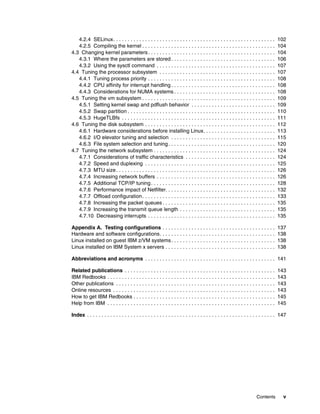
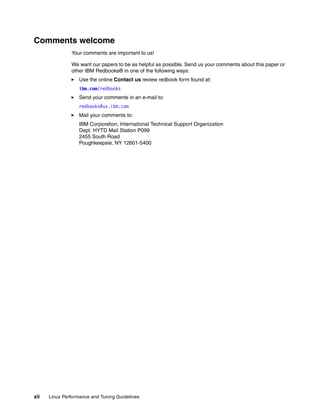
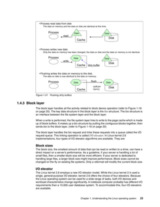
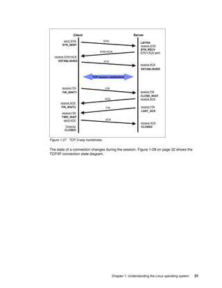
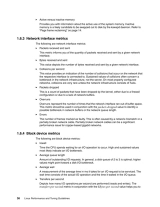
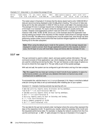
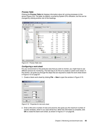
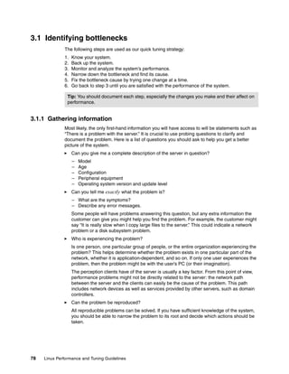
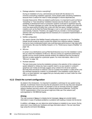
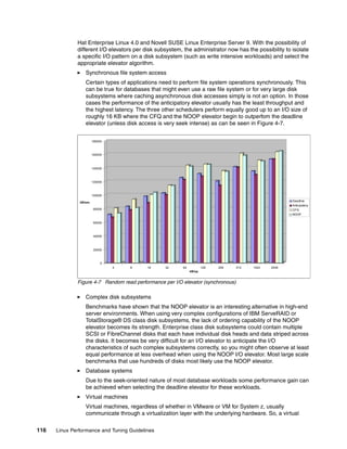
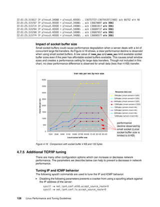
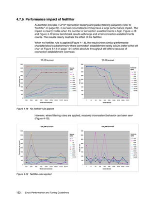
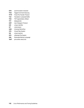
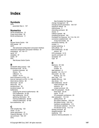
1.1.9 Linux CPU scheduler
The basic functionality of any computer is, quite simply, to compute. To be able to compute,
there must be a means to manage the computing resources, or processors, and the
computing tasks, also known as threads or processes. Thanks to the great work of Ingo
Molnar, Linux features a kernel using a O(1) algorithm as opposed to the O(n) algorithm used
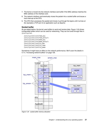
to describe the former CPU scheduler. The term O(1) refers to a static algorithm, meaning
that the time taken to choose a process for placing into execution is constant, regardless of
the number of processes.
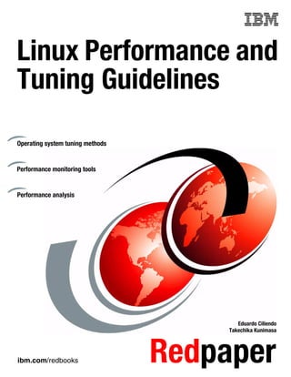
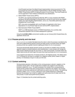
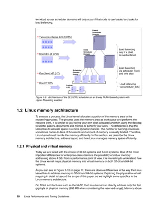
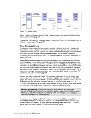
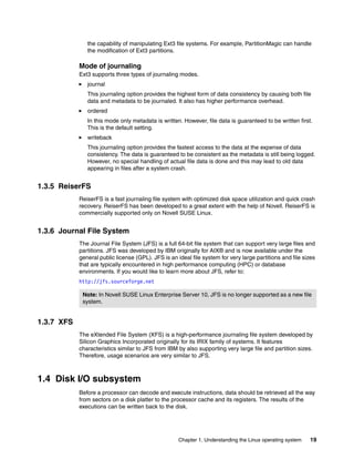
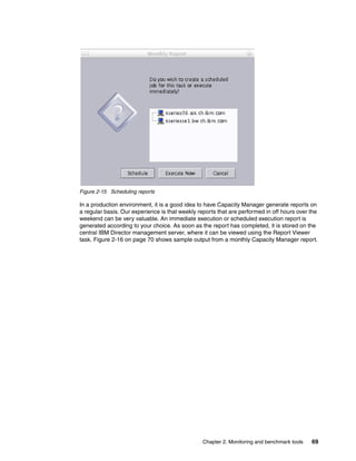
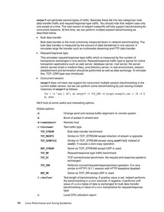
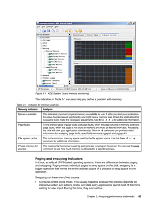
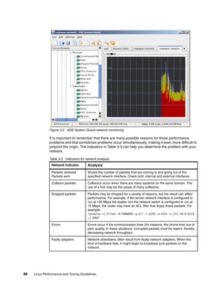
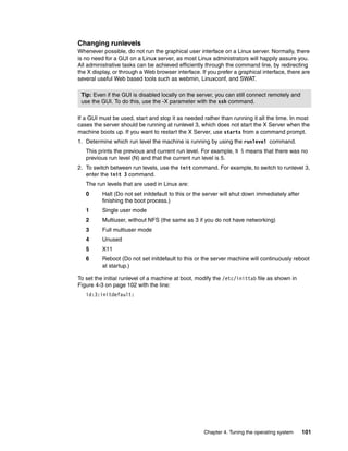
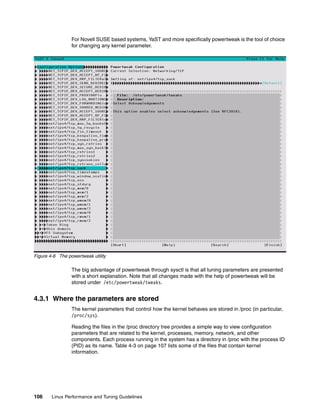
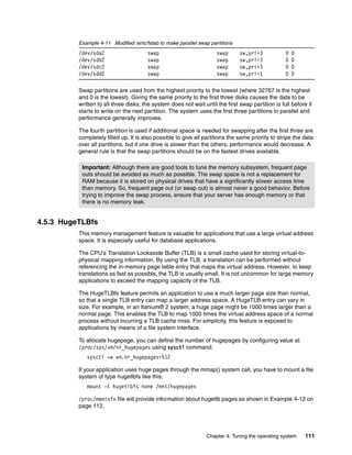
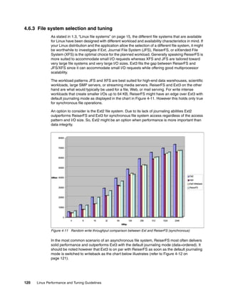
The new scheduler scales very well, regardless of process count or processor count, and
imposes a low overhead on the system. The algorithm uses two process priority arrays:
򐂰 active
򐂰 expired
As processes are allocated a timeslice by the scheduler, based on their priority and prior
blocking rate, they are placed in a list of processes for their priority in the active array. When
they expire their timeslice, they are allocated a new timeslice and placed on the expired array.
When all processes in the active array have expired their timeslice, the two arrays are
switched, restarting the algorithm. For general interactive processes (as opposed to real-time
processes) this results in high-priority processes, which typically have long timeslices, getting
more compute time than low-priority processes, but not to the point where they can starve the
low-priority processes completely. The advantage of such an algorithm is the vastly improved
scalability of the Linux kernel for enterprise workloads that often include vast amounts of
threads or processes and also a significant number of processors. The new O(1) CPU
scheduler was designed for kernel 2.6 but backported to the 2.4 kernel family. Figure 1-8 on
page 9 illustrates how the Linux CPU scheduler works.
Figure 1-8 Linux kernel 2.6 O(1) scheduler
Another significant advantage of the new scheduler is the support for Non-Uniform Memory
Architecture (NUMA) and symmetric multithreading processors, such as Intel®
Hyper-Threading technology.
The improved NUMA support ensures that load balancing will not occur across NUMA nodes
unless a node gets overburdened. This mechanism ensures that traffic over the comparatively
slow scalability links in a NUMA system are minimized. Although load balancing across
processors in a scheduler domain group will be load balanced with every scheduler tick,
priority0
:
priority 139
priority0
:
priority 139
P
P P P
active
expired
array[0]
array[1]
P P
:
:
P P P
priority0
:
priority 139
priority0
:
priority 139
P
P P P
active
expired
array[0]
array[1]
P P
:
:
P P P

24. 10 Linux Performance and Tuning Guidelines
workload across scheduler domains will only occur if that node is overloaded and asks for
load balancing.
Figure 1-9 Architecture of the O(1) CPU scheduler on an 8-way NUMA based system with
Hyper-Threading enabled
1.2 Linux memory architecture
To execute a process, the Linux kernel allocates a portion of the memory area to the
requesting process. The process uses the memory area as workspace and performs the
required work. It is similar to you having your own desk allocated and then using the desktop
to scatter papers, documents and memos to perform your work. The difference is that the
kernel has to allocate space in a more dynamic manner. The number of running processes
sometimes comes to tens of thousands and amount of memory is usually limited. Therefore,
Linux kernel must handle the memory efficiently. In this section, we describe the Linux
memory architecture, address layout, and how Linux manages memory space efficiently.
1.2.1 Physical and virtual memory
Today we are faced with the choice of 32-bit systems and 64-bit systems. One of the most
important differences for enterprise-class clients is the possibility of virtual memory
addressing above 4 GB. From a performance point of view, it is interesting to understand how
the Linux kernel maps physical memory into virtual memory on both 32-bit and 64-bit
systems.
As you can see in Figure 1-10 on page 11, there are obvious differences in the way the Linux
kernel has to address memory in 32-bit and 64-bit systems. Exploring the physical-to-virtual
mapping in detail is beyond the scope of this paper, so we highlight some specifics in the
Linux memory architecture.
On 32-bit architectures such as the IA-32, the Linux kernel can directly address only the first
gigabyte of physical memory (896 MB when considering the reserved range). Memory above
ƒ Two node xSeries 445 (8 CPU)
ƒ One CEC (4 CPU)
ƒ One Xeon MP (HT)
ƒ One HT CPU
Parent
Scheduler
Domain
Child
Scheduler
Domain
Scheduler
Domain
Group
Logical
CPU
Load balancing
only if a child
is overburdened
Load balancing
via scheduler_tick()
and time slice
Load balancing
via scheduler_tick()
1
2
3
…
1
2
3
…
1
2
3
…
1
2
…
1
2
…
1
2
…
1
2
…
1
2
…
1
2
…

25. Chapter 1. Understanding the Linux operating system 11
the so-called ZONE_NORMAL must be mapped into the lower 1 GB. This mapping is
completely transparent to applications, but allocating a memory page in ZONE_HIGHMEM
causes a small performance degradation.
On the other hand, with 64-bit architectures such as x86-64 (also x64), ZONE_NORMAL
extends all the way to 64 GB or to 128 GB in the case of IA-64 systems. As you can see, the
overhead of mapping memory pages from ZONE_HIGHMEM into ZONE_NORMAL can be
eliminated by using a 64-bit architecture.
Figure 1-10 Linux kernel memory layout for 32-bit and 64-bit systems
Virtual memory addressing layout
Figure 1-11 shows the Linux virtual addressing layout for 32-bit and 64-bit architecture.
On 32-bit architectures, the maximum address space that single process can access is 4GB.
This is a restriction derived from 32-bit virtual addressing. In a standard implementation, the
virtual address space is divided into a 3 GB user space and a 1 GB kernel space. There is
some variants like 4 G/4 G addressing layout implementing.
On the other hand, on 64-bit architecture such as x86_64 and ia64, no such restriction exits.
Each single process can benefit from the vast and huge address space.
The Linux Memory Architecture
32-bit Architecture 64-bit Architecture
16 MB
1 GB
64 GB
ZONE_NORMAL
ZONE_DMA
ZONE_HIGHMEM
“Reserved”
128 MB
896 MB
Pages in ZONE_HIGHMEM
must be mapped into
ZONE_NORMAL
1 GB
64 GB
ZONE_DMA
ZONE_NORMAL
~~
~~
Reserved for Kernel
data structures

26. 12 Linux Performance and Tuning Guidelines
Figure 1-11 Virtual memory addressing layout for 32bit and 64-bit architecture
1.2.2 Virtual memory manager
The physical memory architecture of an operating system is usually hidden to the application
and the user because operating systems map any memory into virtual memory. If we want to
understand the tuning possibilities within the Linux operating system, we have to understand
how Linux handles virtual memory. As explained in 1.2.1, “Physical and virtual memory” on
page 10, applications do not allocate physical memory, but request a memory map of a
certain size at the Linux kernel and in exchange receive a map in virtual memory. As you can
see in Figure 1-12, virtual memory does not necessarily have to be mapped into physical
memory. If your application allocates a large amount of memory, some of it might be mapped
to the swap file on the disk subsystem.
Figure 1-12 shows that applications usually do not write directly to the disk subsystem, but
into cache or buffers. The pdflush kernel threads then flushes out data in cache/buffers to the
disk when it has time to do so or if a file size exceeds the buffer cache. Refer to “Flushing a
dirty buffer” on page 22.
32-bit Architecture
64-bit Architecture
3 GB
3 G/1 G kernel
User space Kernel space
0 GB
User space Kernel space
0 GB
4 GB
512 GB or more
x86_64

27. Chapter 1. Understanding the Linux operating system 13
Figure 1-12 The Linux virtual memory manager
Closely connected to the way the Linux kernel handles writes to the physical disk subsystem
is the way the Linux kernel manages disk cache. While other operating systems allocate only
a certain portion of memory as disk cache, Linux handles the memory resource far more
efficiently. The default configuration of the virtual memory manager allocates all available free
memory space as disk cache. Hence it is not unusual to see productive Linux systems that
boast gigabytes of memory but only have 20 MB of that memory free.
In the same context, Linux also handles swap space very efficiently. Swap space being used
does not indicate a memory bottleneck but proves how efficiently Linux handles system
resources. See “Page frame reclaiming” on page 14 for more detail.
Page frame allocation
A page is a group of contiguous linear addresses in physical memory (page frame) or virtual
memory. The Linux kernel handles memory with this page unit. A page is usually 4 K bytes in
size. When a process requests a certain amount of pages, if there are available pages the
Linux kernel can allocate them to the process immediately. Otherwise pages have to be taken
from some other process or page cache. The kernel knows how many memory pages are
available and where they are located.
Buddy system
The Linux kernel maintains its free pages by using a mechanism called a buddy system. The
buddy system maintains free pages and tries to allocate pages for page allocation requests. It
tries to keep the memory area contiguous. If small pages are scattered without consideration,
it might cause memory fragmentation and it’s more difficult to allocate a large portion of pages
into a contiguous area. It could lead to inefficient memory use and performance decline.
Figure 1-13 illustrates how the buddy system allocates pages.
Standard
C Library
(glibc)
Kernel
Subsystems
sh
httpd
mozilla
kswapd
bdflush
Slab Allocator
zoned
buddy
allocator
MMU
VM Subsystem
Disk Driver
User Space
Processes Disk
Physical
Memory

28. 14 Linux Performance and Tuning Guidelines
Figure 1-13 Buddy System
When the attempt of pages allocation fails, the page reclaiming is activated. Refer to “Page
frame reclaiming” on page 14.
You can find information on the buddy system through /proc/buddyinfo. For details, refer to
“Memory used in a zone” on page 47.
Page frame reclaiming
If pages are not available when a process requests to map a certain amount of pages, the
Linux kernel tries to get pages for the new request by releasing certain pages (which were
used before but are not used anymore and are still marked as active pages based on certain
principles) and allocating the memory to a new process. This process is called page
reclaiming. kswapd kernel thread and try_to_free_page() kernel function are responsible for
page reclaiming.
While kswapd is usually sleeping in task interruptible state, it is called by the buddy system
when free pages in a zone fall short of a threshold. It tries to find the candidate pages to be
taken out of active pages based on the Least Recently Used (LRU) principle. The pages least
recently used should be released first. The active list and the inactive list are used to maintain
the candidate pages. kswapd scans part of the active list and check how recently the pages
were used and the pages not used recently are put into the inactive list. You can take a look at
how much memory is considered as active and inactive using the vmstat -a command. For
detail refer to 2.3.2, “vmstat” on page 42.
kswapd also follows another principle. The pages are used mainly for two purposes: page
cache and process address space. The page cache is pages mapped to a file on disk. The
pages that belong to a process address space (called anonymous memory because it is not
mapped to any files, and it has no name) are used for heap and stack. Refer to 1.1.8,
“Process memory segments” on page 8. When kswapd reclaims pages, it would rather shrink
the page cache than page out (or swap out) the pages owned by processes.
A large proportion of page cache that is reclaimed and process address space that is
reclaimed might depend on the usage scenario and will affect performance. You can take
some control of this behavior by using /proc/sys/vm/swappiness. Refer to 4.5.1, “Setting
kernel swap and pdflush behavior” on page 109 for tuning details.
Page out and swap out: The phrases “page out” and “swap out” are sometimes
confusing. The phrase “page out” means take some pages (a part of entire address space)
into swap space while “swap out” means taking entire address space into swap space.
They are sometimes used interchangeably.
Used
Used
Used
Used
Used
Request
for 2 pages Used
4 pages
chunk
Used
Request
for 2 pages
Used
2 pages
chunk
Used
Used
8 pages
chunk
Used
Release
2 pages
Used
2 pages
chunk
8 pages
chunk
8 pages
chunk

29. Chapter 1. Understanding the Linux operating system 15
swap
As we stated before, when page reclaiming occurs, the candidate pages in the inactive list
which belong to the process address space may be paged out. Having swap itself is not
problematic situation. While swap is nothing more than a guarantee in case of over allocation
of main memory in other operating systems, Linux uses swap space far more efficiently. As
you can see in Figure 1-12 on page 13, virtual memory is composed of both physical memory
and the disk subsystem or the swap partition. If the virtual memory manager in Linux realizes
that a memory page has been allocated but not used for a significant amount of time, it moves
this memory page to swap space.
Often you will see daemons such as getty that will be launched when the system starts up but
will hardly ever be used. It appears that it would be more efficient to free the expensive main
memory of such a page and move the memory page to swap. This is exactly how Linux
handles swap, so there is no need to be alarmed if you find the swap partition filled to 50%.
The fact that swap space is being used does not indicate a memory bottleneck; instead it
proves how efficiently Linux handles system resources.
1.3 Linux file systems
One of the great advantages of Linux as an open source operating system is that it offers
users a variety of supported file systems. Modern Linux kernels can support nearly every file
system ever used by a computer system, from basic FAT support to high performance file
systems such as the journaling file system (JFS). However, because Ext2, Ext3, and
ReiserFS are native Linux file systems supported by most Linux distributions (ReiserFS is
commercially supported only on Novell SUSE Linux), we will focus on their characteristics
and give only an overview of the other frequently used Linux file systems.
For more information on file systems and the disk subsystem, see 4.6, “Tuning the disk
subsystem” on page 112.
1.3.1 Virtual file system
Virtual Files System (VFS) is an abstraction interface layer that resides between the user
process and various types of Linux file system implementations. VFS provides common
object models (such as i-node, file object, page cache, directory entry, and so on) and
methods to access file system objects. It hides the differences of each file system
implementation from user processes. Thanks to VFS, user processes do not need to know
which file system to use, or which system call should be issued for each file system.
Figure 1-14 on page 16 illustrates the concept of VFS.

30. 16 Linux Performance and Tuning Guidelines
Figure 1-14 VFS concept
1.3.2 Journaling
In a non-journaling file system, when a write is performed to a file system the Linux kernel
makes changes to the file system metadata first and then writes actual user data next. This
operation sometimes causes higher chances of losing data integrity. If the system suddenly
crashes for some reason while the write operation to file system metadata is in process, the
file system consistency may be broken. fsck fixes the inconsistency by checking all the
metadata and recover the consistency at the time of next reboot. But when the system has a
large volume, it takes a lot of time to be completed. The system is not operational during this
process.
A Journaling file system solves this problem by writing data to be changed to the area called
the journal area before writing the data to the actual file system. The journal area can be
placed both in the file system or out of the file system. The data written to the journal area is
called the journal log. It includes the changes to file system metadata and the actual file data
if supported.
Because journaling writes journal logs before writing actual user data to the file system, it can
cause performance overhead compared to no-journaling file system. How much performance
overhead is sacrificed to maintain higher data consistency depends on how much information
is written to disk before writing user data. We will discuss this topic in 1.3.4, “Ext3” on
page 18.
Figure 1-15 Journaling concept
VFS
System call
User Process cp
open(), read(), write()
translation for each file system
ext2 ext3 Reiserfs
NFS
XFS JFS
AFS VFAT proc
1. write journal logs
File system
Journal area
2. Make changes to actual
file system
3. delete journal logs
write

31. Chapter 1. Understanding the Linux operating system 17
1.3.3 Ext2
The extended 2 file system is the predecessor of the extended 3 file system. A fast, simple file
system, it features no journaling capabilities, unlike most other current file systems.
Figure 1-16 shows the Ext2 file system data structure. The file system starts with the boot
sector and is followed by block groups. Splitting the entire file system into several small block
groups contributes to performance gain because the i-node table and data blocks which hold
user data can reside closer on the disk platter, so seek time can be reduced. A block group
consists of these items:
Super block Information on the file system is stored here. The exact copy of a
super block is placed in the top of every block group.
Block group descriptorInformation on the block group is stored here.
Data block bitmaps Used for free data block management
i-node bitmaps Used for free i-node management
i-node tables i-node tables are stored here. Every file has a corresponding i-node
table which holds meta-data of the file such as file mode, uid, gid,
atime, ctime, mtime, dtime, and pointer to the data block.
Data blocks Where actual user data is stored
Figure 1-16 Ext2 file system data structure
To find data blocks which consist of a file, the kernel searches the i-node of the file first. When
a request to open /var/log/messages comes from a process, the kernel parses the file path
and searches a directory entry of / (root directory) which has the information about files and
directories under itself (root directory). Then the kernel can find the i-node of /var next and
look at the directory entry of /var. It also has the information of files and directories under
itself. The kernel gets down to the file in same manner until it finds i-node of the file. The Linux
Ext2
boot sector
boot sector
BLOCK
GROUP 0
BLOCK
GROUP 0
BLOCK
GROUP 1
BLOCK
GROUP 1
BLOCK
GROUP 2
BLOCK
GROUP 2
:
:
:
:
BLOCK
GROUP N
BLOCK
GROUP N
super block
super block
block group
descriptors
block group
descriptors
data-block
bitmaps
data block
bitmaps
inode
bitmaps
i-node
bitmaps
inode-table
i-node table
Data-blocks
data blocks

32. 18 Linux Performance and Tuning Guidelines
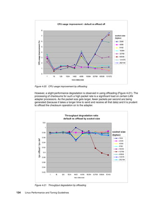
kernel uses a file object cache such as directory entry cache or i-node cache to accelerate
finding the corresponding i-node.
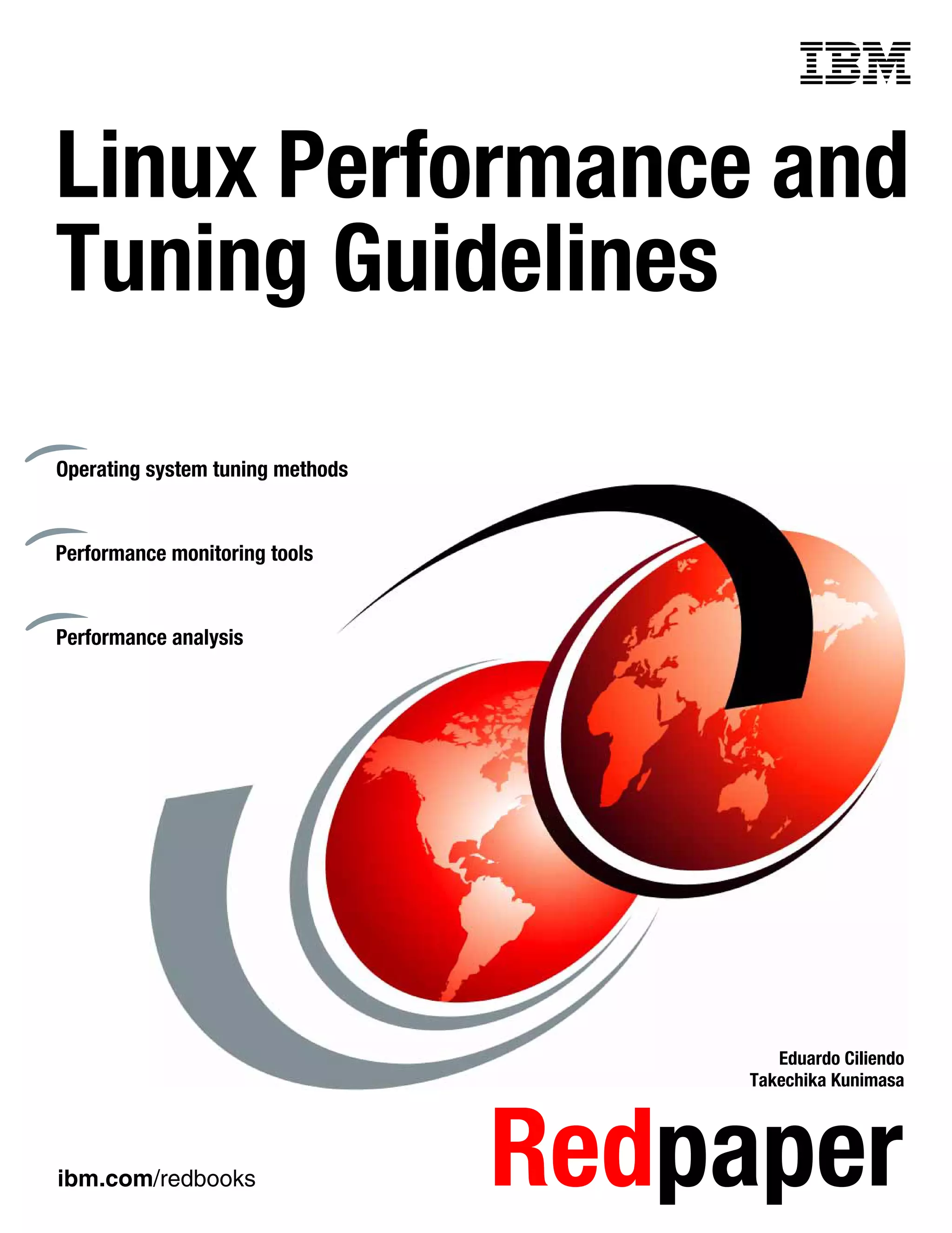
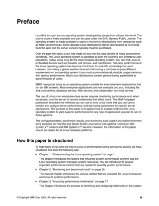
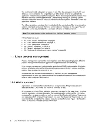
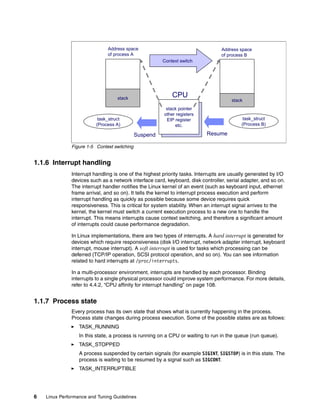
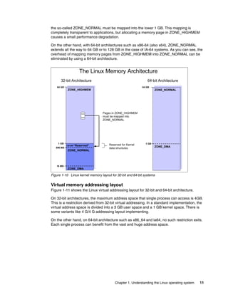
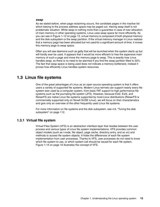
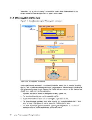
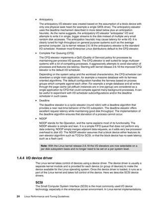
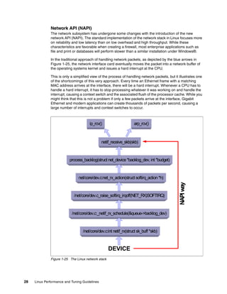
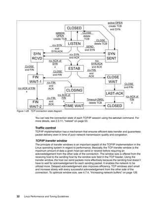
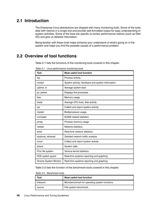
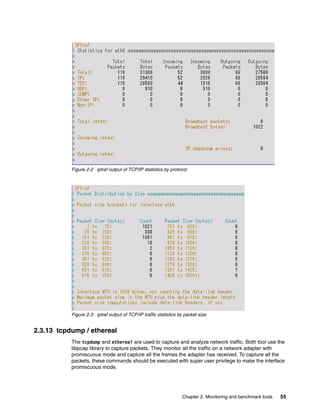
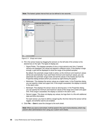
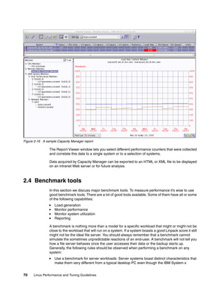
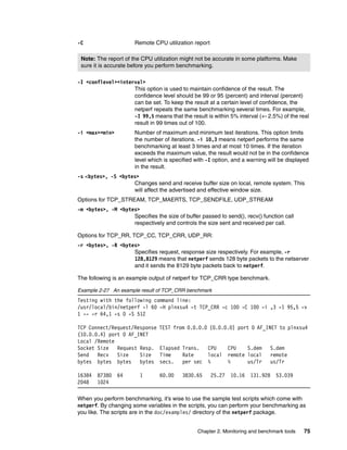
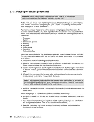
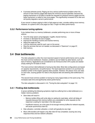
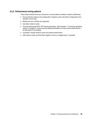
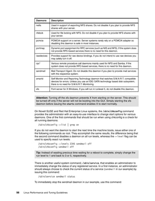
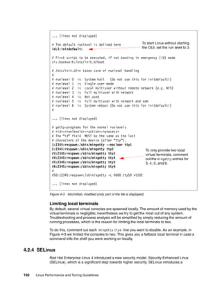
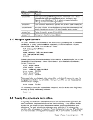
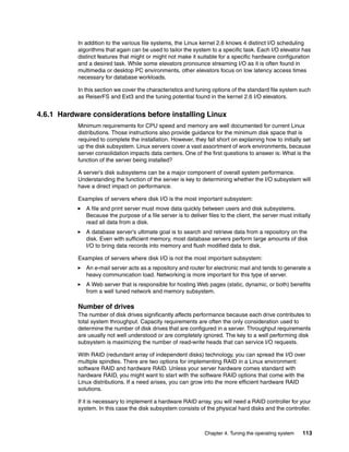
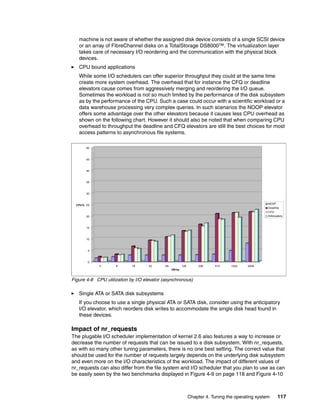
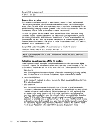
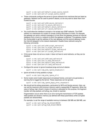
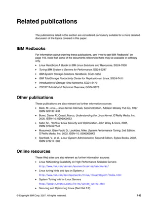
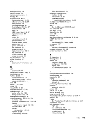
Once the Linux kernel knows the i-node of the file, it tries to reach the actual user data block.
As we described, i-node has the pointer to the data block. By referring to it, the kernel can get
to the data block. For large files, Ext2 implements direct/indirect references to the data block.
Figure 1-17 illustrates how it works.
Figure 1-17 Ext2 file system direct / indirect reference to data block
The file system structure and file access operations differ by file systems. This gives each
files system different characteristics.
1.3.4 Ext3
The current Enterprise Linux distributions support the extended 3 file system. This is an
updated version of the widely used extended 2 file system. Though the fundamental
structures are similar to the Ext2 file system, the major difference is the support of journaling
capability. Highlights of this file system include:
򐂰 Availability: Ext3 always writes data to the disks in a consistent way, so in case of an
unclean shutdown (unexpected power failure or system crash), the server does not have
to spend time checking the consistency of the data, thereby reducing system recovery
from hours to seconds.
򐂰 Data integrity: By specifying the journaling mode data=journal on the mount command, all
data, both file data and metadata, is journaled.
򐂰 Speed: By specifying the journaling mode data=writeback, you can decide on speed
versus integrity to meet the needs of your business requirements. This will be notable in
environments where there are heavy synchronous writes.
򐂰 Flexibility: Upgrading from existing Ext2 file systems is simple, and no reformatting is
necessary. By executing the tune2fs command and modifying the /etc/fstab file, you can
easily update an Ext2 to an Ext3 file system. Also note that Ext3 file systems can be
mounted as Ext2 with journaling disabled. Products from many third-party vendors have
ext2 disk i-node
i_blocks[2]
i_blocks[12]
i_blocks[13]
i_blocks[14]
i_blocks[3]
i_blocks[4]
i_blocks[0]
i_blocks[1]
i_size
：
i_blocks
i_blocks[6]
i_blocks[7]
i_blocks[8]
i_blocks[9]
i_blocks[10]
i_blocks[11]
Data
block
Indirect
block
Indirect
block
Indirect
block
Indirect
block
i_blocks[5]
direct
indirect
double indirect
trebly indirect
Indirect
block
Indirect
block
Data
block
Indirect
block
Indirect
block
Data
block
Indirect
block
Indirect
block
Indirect
block
Indirect
block
Data
block

33. Chapter 1. Understanding the Linux operating system 19
the capability of manipulating Ext3 file systems. For example, PartitionMagic can handle
the modification of Ext3 partitions.
Mode of journaling
Ext3 supports three types of journaling modes.
򐂰 journal
This journaling option provides the highest form of data consistency by causing both file
data and metadata to be journaled. It also has higher performance overhead.
򐂰 ordered
In this mode only metadata is written. However, file data is guaranteed to be written first.
This is the default setting.
򐂰 writeback
This journaling option provides the fastest access to the data at the expense of data
consistency. The data is guaranteed to be consistent as the metadata is still being logged.
However, no special handling of actual file data is done and this may lead to old data
appearing in files after a system crash.
1.3.5 ReiserFS
ReiserFS is a fast journaling file system with optimized disk space utilization and quick crash
recovery. ReiserFS has been developed to a great extent with the help of Novell. ReiserFS is
commercially supported only on Novell SUSE Linux.
1.3.6 Journal File System
The Journal File System (JFS) is a full 64-bit file system that can support very large files and
partitions. JFS was developed by IBM originally for AIX® and is now available under the
general public license (GPL). JFS is an ideal file system for very large partitions and file sizes
that are typically encountered in high performance computing (HPC) or database
environments. If you would like to learn more about JFS, refer to:
http://jfs.sourceforge.net
1.3.7 XFS
The eXtended File System (XFS) is a high-performance journaling file system developed by
Silicon Graphics Incorporated originally for its IRIX family of systems. It features
characteristics similar to JFS from IBM by also supporting very large file and partition sizes.
Therefore, usage scenarios are very similar to JFS.
1.4 Disk I/O subsystem
Before a processor can decode and execute instructions, data should be retrieved all the way
from sectors on a disk platter to the processor cache and its registers. The results of the
executions can be written back to the disk.
Note: In Novell SUSE Linux Enterprise Server 10, JFS is no longer supported as a new file
system.

34. 20 Linux Performance and Tuning Guidelines
We’ll take a look at the Linux disk I/O subsystem to have a better understanding of the
components which have a major effect on system performance.
1.4.1 I/O subsystem architecture
Figure 1-18 shows basic concept of I/O subsystem architecture
Figure 1-18 I/O subsystem architecture
For a quick overview of overall I/O subsystem operations, we will use an example of writing
data to a disk. The following sequence outlines the fundamental operations that occur when a
disk-write operation is performed. Assume that the file data is on sectors on disk platters, has
already been read, and is on the page cache.
1. A process requests to write a file through the write() system call.
2. The kernel updates the page cache mapped to the file.
3. A pdflush kernel thread takes care of flushing the page cache to disk.
4. The file system layer puts each block buffer together to a bio struct (refer to 1.4.3, “Block
layer” on page 23) and submits a write request to the block device layer.
5. The block device layer gets requests from upper layers and performs an I/O elevator
operation and puts the requests into the I/O request queue.
device driver
block layer
VFS / file system layer
file
disk device
I/O Request queue
User process
sector
block buffer
bio
page cache page
cache
page
cache
Device driver
Disk
write()
pdflush
I/O scheduler

35. Chapter 1. Understanding the Linux operating system 21
6. A device driver such as SCSI or other device specific drivers will take care of write
operation.
7. A disk device firmware performs hardware operations like seek head, rotation, and data
transfer to the sector on the platter.
1.4.2 Cache
In the last 20 years, the performance improvement of processors has outperformed that of the
other components in a computer system such as processor cache, bus, RAM, disk, and so
on. Slower access to memory and disk restricts overall system performance, so system
performance is not enhanced by processor speed improvement. The cache mechanism
resolves this problem by caching frequently used data in faster memory. It reduces the
chances of having to access slower memory. Current computer systems use this technique in
almost all I/O components such as hard disk drive cache, disk controller cache, file system
cache, cache handled by each application, and so on.
Memory hierarchy
Figure 1-19 shows the concept of memory hierarchy. As the difference of access speed
between the CPU register and disk is large, the CPU will spend more time waiting for data
from slow disk devices, and therefore it significantly reduces the advantage of a fast CPU.
Memory hierarchal structure reduces this mismatch by placing L1 cache, L2 cache, RAM and
some other caches between the CPU and disk. It enables a process to get less chance to
access slower memory and disk. The memory closer to the processor has higher speed and
less size.
This technique can also take advantage of locality of reference principle. The higher the
cache hit rate on faster memory is, the faster the access to data.
Figure 1-19 Memory hierarchy
Locality of reference
As we stated previously in “Memory hierarchy” achieving higher cache hit rate is the key for
performance improvement. To achieve higher cache hit rate, the technique called “locality of
reference” is used. This technique is based on the following principles:
򐂰 The data most recently used has a high probability of being used in the near future
(temporal locality).
򐂰 The data that resides close to the data which has been used has a high probability of
being used (spatial locality).
Figure 1-20 on page 22 illustrates this principle.
CPU register
CPU
cache
register RAM
very fast very slow
Large
speed mismatch
very fast
fast
Disk
slow very slow
Disk

36. 22 Linux Performance and Tuning Guidelines
Figure 1-20 Locality of reference
Linux uses this principle in many components such as page cache, file object cache (i-node
cache, directory entry cache, and so on), read ahead buffer and more.
Flushing a dirty buffer
When a process reads data from disk, the data is copied to memory. The process and other
processes can retrieve the same data from the copy of the data cached in memory. When a
process tries to change the data, the process changes the data in memory first. At this time,
the data on disk and the data in memory is not identical and the data in memory is referred to
as a dirty buffer. The dirty buffer should be synchronized to the data on disk as soon as
possible, or the data in memory could be lost if a sudden crash occurs.
The synchronization process for a dirty buffer is called flush. In the Linux kernel 2.6
implementation, pdflush kernel thread is responsible for flushing data to the disk. The flush
occurs on a regular basis (kupdate) and when the proportion of dirty buffers in memory
exceeds a certain threshold (bdflush). The threshold is configurable in the
/proc/sys/vm/dirty_background_ratio file. For more information, refer to 4.5.1, “Setting
kernel swap and pdflush behavior” on page 109.
Temporal locality Spatial locality
CPU
Register
Cache
Memory
Disk
First access
Data
Data
Data
Data
Second access in a few seconds Second access to data2 in a few seconds
Data2
Data2
CPU
Register
Cache
Memory
Disk
Data
Data
Data
Data
CPU
Register
Cache
Memory
Disk
First access
Data1
Data1
Data
Data
Data2
Data2
CPU
Register
Cache
Memory
Disk
Data1
Data1
Data
Data

37. Chapter 1. Understanding the Linux operating system 23
Figure 1-21 Flushing dirty buffers
1.4.3 Block layer
The block layer handles all the activity related to block device operation (refer to Figure 1-18
on page 20). The key data structure in the block layer is the bio structure. The bio structure is
an interface between the file system layer and the block layer.
When a write is performed, the file system layer tries to write to the page cache which is made
up of block buffers. It makes up a bio structure by putting the contiguous blocks together, then
sends bio to the block layer. (refer to Figure 1-18 on page 20)
The block layer handles the bio request and links these requests into a queue called the I/O
request queue. This linking operation is called I/O elevator. In Linux kernel 2.6
implementations, four types of I/O elevator algorithms are available. They are:
Block sizes
The block size, the smallest amount of data that can be read or written to a drive, can have a
direct impact on a server’s performance. As a guideline, if your server is handling a lot of
small files, then a smaller block size will be more efficient. If your server is dedicated to
handling large files, a larger block size might improve performance. Block sizes cannot be
changed on the fly on existing file systems. Only a reformat will modify the current block size.
I/O elevator
The Linux kernel 2.6 employs a new I/O elevator model. While the Linux kernel 2.4 used a
single, general-purpose I/O elevator, kernel 2.6 offers the choice of four elevators. Because
the Linux operating system can be used for a wide range of tasks, both I/O devices and
workload characteristics change significantly. A notebook computer probably has different I/O
requirements than a 10,000 user database system. To accommodate this, four I/O elevators
are available.
Process
Cache
Data
Disk
Data
read
Process
Cache
Disk
Data
write
Data
dirty buffer
•Process read data from disk
The data on memory and the data on disk are identical at this time.
•Process writes new data
Only the data on memory has been changed, the data on disk and the data on memory is not identical.
Process
Cache
Disk
Data
flush
•Flushing writes the data on memory to the disk.
The data on disk is now identical to the data on memory.
Data
•pdflush
•sync()

38. 24 Linux Performance and Tuning Guidelines
򐂰 Anticipatory
The anticipatory I/O elevator was created based on the assumption of a block device with
only one physical seek head (for example a single SATA drive). The anticipatory elevator
uses the deadline mechanism described in more detail below plus an anticipation
heuristic. As the name suggests, the anticipatory I/O elevator “anticipates” I/O and
attempts to write it in single, bigger streams to the disk instead of multiple very small
random disk accesses. The anticipation heuristic may cause latency for write I/O. It is
clearly tuned for high throughput on general purpose systems such as the average
personal computer. Up to kernel release 2.6.18 the anticipatory elevator is the standard
I/O scheduler. However most Enterprise Linux distributions default to the CFQ elevator.
򐂰 Complete Fair Queuing (CFQ)
The CFQ elevator implements a QoS (Quality of Service) policy for processes by
maintaining per-process I/O queues. The CFQ elevator is well suited for large multiuser
systems with a lot of competing processes. It aggressively attempts to avoid starvation of
processes and features low latency. Starting with kernel release 2.6.18 the improved CFQ
elevator is the default I/O scheduler.
Depending on the system setup and the workload characteristics, the CFQ scheduler can
slowdown a single main application, for example a massive database with its fairness
oriented algorithms. The default configuration handles the fairness based on process
groups which compete against each other. For example a single database and all writes
through the page cache (all pdflush instances are in one pgroup) are considered as a
single application by CFQ that could compete against many background processes. It can
be useful to experiment with I/O scheduler subconfigurations and/or the deadline
scheduler in such cases.
򐂰 Deadline
The deadline elevator is a cyclic elevator (round robin) with a deadline algorithm that
provides a near real-time behavior of the I/O subsystem. The deadline elevator offers
excellent request latency while maintaining good disk throughput. The implementation of
the deadline algorithm ensures that starvation of a process cannot occur.
򐂰 NOOP
NOOP stands for No Operation, and the name explains most of its functionality. The
NOOP elevator is simple and lean. It is a simple FIFO queue that does not perform any
data ordering. NOOP simply merges adjacent data requests, so it adds very low processor
overhead to disk I/O. The NOOP elevator assumes that a block device either features its
own elevator algorithm such as TCQ for SCSI, or that the block device has no seek latency
such as a flash card.
1.4.4 I/O device driver
The Linux kernel takes control of devices using a device driver. The device driver is usually a
separate kernel module and is provided for each device (or group of devices) to make the
device available for the Linux operating system. Once the device driver is loaded, it runs as a
part of the Linux kernel and takes full control of the device. Here we describe SCSI device
drivers.
SCSI
The Small Computer System Interface (SCSI) is the most commonly used I/O device
technology, especially in the enterprise server environment. In Linux kernel implementations,
Note: With the Linux kernel release 2.6.18 the I/O elevators are now selectable on a
per disk subsystem basis and no longer need to be set on a per system level.

39. Chapter 1. Understanding the Linux operating system 25
SCSI devices are controlled by device driver modules. They consist of the following types of
modules.
򐂰 Upper level drivers: sd_mod, sr_mod (SCSI-CDROM), st (SCSI Tape), sq (SCSI generic
device), and so on.
Provide functionalities to support several types of SCSI devices such as SCSI CD-ROM,
SCSI tape, and so on.
򐂰 Middle level driver: scsi_mod
Implements SCSI protocol and common SCSI functionality.
򐂰 Low level drivers
Provide lower level access to each device. Low level driver is basically specific to a
hardware device and provided for each device. For example, ips for IBM ServeRAID™
controller, qla2300 for Qlogic HBA, mptscsih for LSI Logic SCSI controller, and so on.
򐂰 Pseudo driver: ide-scsi
Used for IDE-SCSI emulation.
Figure 1-22 Structure of SCSI drivers
If specific functionality is implemented for a device, it should be implemented in device
firmware and the low level device driver. The supported functionality depends on which
hardware you use and which version of device driver you use. The device itself should also
support the desired functionality. Specific functions are usually tuned by a device driver
parameter. You can try some performance tuning in /etc/modules.conf. Refer to the device
and device driver documentation for tuning hints and tips.
1.4.5 RAID and storage system
The selection and configuration of storage system and RAID types are also important factors
in terms of system performance. Linux supports software RAID, but the details of this topic
are out of scope of this paper. We include some of the tuning considerations in 4.6.1,
“Hardware considerations before installing Linux” on page 113.
For more details of the available IBM storage solutions, see:
򐂰 Tuning IBM System x Servers for Performance, SG24-5287
򐂰 IBM System Storage Solutions Handbook, SG24-5250
򐂰 Introduction to Storage Area Networks, SG24-5470
ips qla2300
mptscsih
st sr_mod
sd_mod
sg
scsi_mod
……
Upper level driver
Mid level driver
Device
Process
Low level driver

40. 26 Linux Performance and Tuning Guidelines
1.5 Network subsystem
The network subsystem is another important subsystem in the performance perspective.
Networking operations interact with many components other than Linux such as switches,
routers, gateways, PC clients, and so on. Though these components might be out of the
control of Linux, they have a lot of influence on the overall performance. Keep in mind that you
have to work closely with people working on the network system.
Here we mainly focus on how Linux handles networking operations.
1.5.1 Networking implementation
The TCP/IP protocol has a layered structure similar to the OSI layer model. The Linux kernel
networking implementation employs a similar approach. Figure 1-23 illustrates the layered
Linux TCP/IP stack and provides an overview of TCP/IP communication.
Figure 1-23 Network layered structure and overview of networking operation
Linux uses a socket interface for TCP/IP networking operation as many UNIX systems do.
The socket provides an interface for user applications. We will look at the sequence that
outlines the fundamental operations that occur during network data transfer.
1. When an application sends data to its peer host, the application creates its data.
2. The application opens the socket and writes the data through the socket interface.
3. The socket buffer is used to deal with the transferred data. The socket buffer has reference
to the data and it goes down through the layers.
4. In each layer, appropriate operations such as parsing the headers, adding and modifying
the headers, check sums, routing operation, fragmentation, and so on are performed.
When the socket buffer goes down through the layers, the data itself is not copied between
the layers. Because copying actual data between different layers is not effective, the kernel
avoids unnecessary overhead by just changing the reference in the socket buffer and
passing it to the next layer.
5. Finally, the data goes out to the wire from the network interface card.
6. The Ethernet frame arrives at the network interface of the peer host.
IP
TCP/UDP
INET socket
BSD socket
Device
Datalink
Device driver
NIC
Process
sk_buff
Ethernet
Header
IP Header
TCP/UDP
Header
Data
IP
TCP/UDP
INET socket
BSD socket
Device
Datalink
Device driver
NIC
Process

41. Chapter 1. Understanding the Linux operating system 27
7. The frame is moved into the network interface card buffer if the MAC address matches the
MAC address of the interface card.
8. The network interface card eventually moves the packet into a socket buffer and issues a
hard interrupt at the CPU.
9. The CPU then processes the packet and moves it up through the layers until it arrives at
(for example) a TCP port of an application such as Apache.
Socket buffer
As we stated before, the kernel uses buffers to send and receive data. Figure 1-24 shows
configurable buffers which can be used for networking. They can be tuned through files in
/proc/sys/net.
/proc/sys/net/core/rmem_max
/proc/sys/net/core/rmem_default
/proc/sys/net/core/wmem_max
/proc/sys/net/core/wmem_default
/proc/sys/net/ipv4/tcp_mem
/proc/sys/net/ipv4/tcp_rmem
/proc/sys/net/ipv4/tcp_wmem
Sometimes it might have an effect on the network performance. We’ll cover the details in
4.7.4, “Increasing network buffers” on page 126.
Figure 1-24 socket buffer memory allocation
tcp_mem
tcp_mem
tcp_mem
socket
tcp_wmem
receive
buffer
send
buffer
socket
socket
socket
tcp_rmem
r s
r s
socket
r s
send
buffer
receive
buffer
rmem_max wmem_max
IPX
Appletalk
TCP/IP

42. 28 Linux Performance and Tuning Guidelines
Network API (NAPI)
The network subsystem has undergone some changes with the introduction of the new
network API (NAPI). The standard implementation of the network stack in Linux focuses more
on reliability and low latency than on low overhead and high throughput. While these
characteristics are favorable when creating a firewall, most enterprise applications such as
file and print or databases will perform slower than a similar installation under Windows®.
In the traditional approach of handling network packets, as depicted by the blue arrows in
Figure 1-25, the network interface card eventually moves the packet into a network buffer of
the operating systems kernel and issues a hard interrupt at the CPU.
This is only a simplified view of the process of handling network packets, but it illustrates one
of the shortcomings of this very approach. Every time an Ethernet frame with a matching
MAC address arrives at the interface, there will be a hard interrupt. Whenever a CPU has to
handle a hard interrupt, it has to stop processing whatever it was working on and handle the
interrupt, causing a context switch and the associated flush of the processor cache. While you
might think that this is not a problem if only a few packets arrive at the interface, Gigabit
Ethernet and modern applications can create thousands of packets per second, causing a
large number of interrupts and context switches to occur.
Figure 1-25 The Linux network stack
DEVICE
/net/core/dev.c:_netif_rx_schedule(&queue->backlog_dev)
/net/core/dev.c:int netif_rx(struct sk_buff *skb)
/net/core/dev.c_raise_softirq_irqoff(NET_RX)SOFTIRQ)
net/core/dev.c:net_rx_action(struct softirq_action*h)
process_backlog(struct net_device*backlog_dev, int *budget)
netif_receive_skb(skb)
ip_rcv() arp_rcv()
NAPI
way
DEVICE
/net/core/dev.c:_netif_rx_schedule(&queue->backlog_dev)
/net/core/dev.c:int netif_rx(struct sk_buff *skb)
/net/core/dev.c_raise_softirq_irqoff(NET_RX)SOFTIRQ)
net/core/dev.c:net_rx_action(struct softirq_action*h)
process_backlog(struct net_device*backlog_dev, int *budget)
netif_receive_skb(skb)
ip_rcv() arp_rcv()
NAPI
way

43. Chapter 1. Understanding the Linux operating system 29
Because of this, NAPI was introduced to counter the overhead associated with processing
network traffic. For the first packet, NAPI works just like the traditional implementation as it
issues an interrupt for the first packet. But after the first packet, the interface goes into a
polling mode. As long as there are packets in the DMA ring buffer of the network interface, no
new interrupts will be caused, effectively reducing context switching and the associated
overhead. Should the last packet be processed and the ring buffer be emptied, then the
interface card will again fall back into the interrupt mode. NAPI also has the advantage of
improved multiprocessor scalability by creating soft interrupts that can be handled by multiple
processors. While NAPI would be a huge improvement for most enterprise class
multiprocessor systems, it requires NAPI-enabled drivers. There is significant room for tuning,
as we will explore in the tuning section of this paper.
Netfilter
Linux has an advanced firewall capability as a part of the kernel. This capability is provided by
Netfilter modules. You can manipulate and configure Netfilter using the iptables utility.
Generally speaking, Netfilter provides the following functions.
򐂰 Packet filtering: If a packet matches a rule, Netfilter accepts or denies the packets or takes
appropriate action based on defined rules.
򐂰 Address translation: If a packet matches a rule, Netfilter alters the packet to meet the
address translation requirements.
Matching filters can be defined with the following properties.
򐂰 Network interface
򐂰 IP address, IP address range, subnet
򐂰 Protocol
򐂰 ICMP Type
򐂰 Port
򐂰 TCP flag
򐂰 State (refer to “Connection tracking” on page 30)
Figure 1-26 give an overview of how packets traverse the Netfilter chains which are the lists of
defined rules applied at each point in sequence.
Figure 1-26 Netfilter packet flow
Netfilter will take appropriate actions if the packet matches the rule. The action is called a
target. Some possible targets are:
PREROUTING
PREROUTING
INPUT
INPUT OUTPUT
OUTPUT
FORWARD
FORWARD POSTROUTING
POSTROUTING
ROUTING
Local process
originated from
local process
incoming
packets
forwarded
packets
Connection Tracking
Mangle
NAT(DNAT)
Filter
Connection Tracking
Filter
Connection Tracking
Mangle
NAT(DNAT)
Filter
Connection Tracking
NAT(SNAT,MASQUERADE)
incoming packets
outgoing
packets

44. 30 Linux Performance and Tuning Guidelines
ACCEPT: Accept the packet and let it through.
DROP: Silently discard the packet.
REJECT: Discard the packet by sending back the packet such as ICMP port
unreachable. TCP reset to originating host.
LOG: Log the matching packet.
MASQUERADE, SNAT, DNAT, REDIRECT:Address translation
Connection tracking
To achieve more sophisticated firewall capability, Netfilter uses the connection tracking
mechanism which keeps track of the state of all network traffic. Using the TCP connection
state (refer to “Connection establishment” on page 30) and other network properties (such as
IP address, port, protocol, sequence number, ack number, ICMP type, and so on), Netfilter
classifies each packet to the following four states.
NEW: packet attempting to establish new connection
ESTABLISHED: packet goes through established connection
RELATED: packet which is related to previous packets
INVALID: packet which is unknown state due to malformed or invalid packet
In addition, Netfilter can use a separate module to perform more detailed connection tracking
by analyzing protocol specific properties and operations. For example, there are connection
tracking modules for FTP, NetBIOS, TFTP, IRC, and so on.
1.5.2 TCP/IP
TCP/IP has been the default network protocol for many years. Linux TCP/IP implementation
is fairly compliant with its standards. For better performance tuning, you should be familiar
with basic TCP/IP networking.
For more details, refer to TCP/IP Tutorial and Technical Overview, GG24-3376.
Connection establishment
Before application data is transferred, the connection should be established between client
and server. The connection establishment process is called TCP/IP 3-way hand shake.
Figure 1-27 on page 31 outlines the basic connection establishment and termination process.
1. A client sends a SYN packet (a packet with SYN flag set) to its peer server to request
connection.
2. The server receives the packet and sends back a SYN+ACK packet.
3. Then the client sends an ACK packet to its peer to complete connection establishment.
Once the connection is established, the application data can be transferred through the
connection. When all data has been transferred, the connection closing process starts.
1. The client sends a FIN packet to the server to start the connection termination process.
2. The server sends the acknowledgement of the FIN back and then sends the FIN packet to
the client if it has no data to send to the client.
3. The client sends an ACK packet to the server to complete connection termination.

45. Chapter 1. Understanding the Linux operating system 31
Figure 1-27 TCP 3-way handshake
The state of a connection changes during the session. Figure 1-28 on page 32 shows the
TCP/IP connection state diagram.
Client Server
SYN_SENT
LISTEN
SYN_RECV
ESTABLISHED
ESTABLISHED
SYN
SYN+ACK
ACK
FIN
ACK
FIN
ACK
TCP session established
FIN_WAIT1
FIN_WAIT2
receive FIN
send SYN
receive SYN
receive SYN+ACK
receive ACK
receive ACK
receive FIN
TIME_WAIT
send ACK
receive ACK
CLOSE_WAIT
receive FIN
LAST_ACK
CLOSED
receive ACK
SYN＋ACK sent
receive FIN
CLOSED
TimeOut

46. 32 Linux Performance and Tuning Guidelines
Figure 1-28 TCP connection state diagram
You can see the connection state of each TCP/IP session using the netstat command. For
more details, see 2.3.11, “netstat” on page 53.
Traffic control
TCP/IP implementation has a mechanism that ensures efficient data transfer and guarantees
packet delivery even in time of poor network transmission quality and congestion.
TCP/IP transfer window
The principle of transfer windows is an important aspect of the TCP/IP implementation in the
Linux operating system in regard to performance. Basically, the TCP transfer window is the
maximum amount of data a given host can send or receive before requiring an
acknowledgement from the other side of the connection. The window size is offered from the
receiving host to the sending host by the window size field in the TCP header. Using the
transfer window, the host can send packets more effectively because the sending host doesn’t
have to wait for acknowledgement for each sending packet. It enables the network to be
utilized more. Delayed acknowledgement also improves efficiency. TCP windows start small
and increase slowly with every successful acknowledgement from the other side of the
connection. To optimize window size, see 4.7.4, “Increasing network buffers” on page 126
CLOSED
LISTEN
SYN
SENT
ESTAB
SYN
RCVD
rcv SYN
snd ACK
FIN
WAIT-1
CLOSE
WAIT
CLOSING
TIME WAIT
FIN
WAIT-2 CLOSED
LAST-ACK
rcv ACK of FIN
x
rcv FIN
snd
ACK
rcv FIN
snd
ACK
rcv ACK of
FIN
x
CLOSE
snd FIN
CLOSE
snd FIN
rcv ACK of
SYN
x
rcv SYN
snd
SYN,ACK
passive
OPEN
create TCB
CLOSE
delete
TCB
SEND
snd SYN
CLOSE
delete TCB
active OPEN
create TCB
snd SYN
rcv
SYN,ACK
snd ACK
rcv FIN
snd
ACK
Timeout=2MSL
delete TCB
CLOSE
snd FIN
rcv ACK of
FIN
x

47. Chapter 1. Understanding the Linux operating system 33
Figure 1-29 Sliding window and delayed ack
As an option, high-speed networks can use a technique called window scaling to increase the
maximum transfer window size even more. We will analyze the effects of these
implementations in more detail in “Tuning TCP options” on page 131.
Retransmission
In the connection establishment and termination and data transfer, many timeouts and data
retransmissions can be caused by various reasons (faulty network interface, slow router,
network congestion, buggy network implementation, and so on). TCP/IP handles this situation
by queuing packets and trying to send packets several times.
You can change some behavior of the kernel by configuring parameters. You might want to
increase the number of attempts for TCP SYN connection establishment packets on the
network with a high rate of packet loss. You can also change some of the timeout thresholds
through files under /proc/sys/net. For more information, see “Tuning TCP behavior” on
page 130.
1.5.3 Offload
If the network adapter on your system supports hardware offload functionality, the kernel can
offload part of its task to the adapter and it can reduce CPU utilization.
򐂰 Checksum offload
IP/TCP/UDP checksum is performed to make sure that the packet is correctly transferred
by comparing the value of the checksum field in protocol headers and the calculated
values by the packet data.
򐂰 TCP segmentation offload (TSO)
When data greater than the supported maximum transmission unit (MTU) is sent to the
network adapter, the data should be divided into MTU sized packets. The adapter takes
care of that on behalf of the kernel.
For information on more advanced network features, refer to Tuning IBM System x Servers for
Performance, SG24-5287. section 10.3. Advanced network features.
Sender Receiver
Sender Receiver
Delayed Ack
Sliding
window

48. 34 Linux Performance and Tuning Guidelines
1.5.4 Bonding module
The Linux kernel provides network interface aggregation capability by using a bonding driver.
This is a device independent bonding driver. (There are also device specific drivers.) The
bonding driver supports the 802.3 link aggregation specification and some original load
balancing and fault tolerant implementations. It achieves a higher level of availability and
performance improvement. Please refer to the kernel documentation
Documentation/networking/bonding.txt.
1.6 Understanding Linux performance metrics
Before we can look at the various tuning parameters and performance measurement utilities
in the Linux operating system, it makes sense to discuss various available metrics and their
meaning in regard to system performance. Because this is an open source operating system,
a lot of performance measurement tools are available. The tool you ultimately choose will
depend upon your personal preference and the amount of data and detail you require. Even
though numerous tools are available, all performance measurement utilities measure the
same metrics, so understanding the metrics enables you to use whatever utility you come
across. Therefore, we cover only the most important metrics. Many more detailed values are
available that might be useful for detailed analysis, but they are beyond the scope of this
paper.
1.6.1 Processor metrics
The following are processor metrics:
򐂰 CPU utilization
This is probably the most straightforward metric. It describes the overall utilization per
processor. On IBM System x architectures, if the CPU utilization exceeds 80% for a
sustained period of time, a processor bottleneck is likely.
򐂰 User time
Depicts the CPU percentage spent on user processes, including nice time. High values in
user time are generally desirable because, in this case, the system performs actual work.
򐂰 System time
Depicts the CPU percentage spent on kernel operations including IRQ and softirq time.
High and sustained system time values can point you to bottlenecks in the network and
driver stack. A system should generally spend as little time as possible in kernel time.
򐂰 Waiting
Total amount of CPU time spent waiting for an I/O operation to occur. Like the blocked
value, a system should not spend too much time waiting for I/O operations; otherwise you
should investigate the performance of the respective I/O subsystem.
򐂰 Idle time
Depicts the CPU percentage the system was idle waiting for tasks.
򐂰 Nice time
Depicts the CPU percentage spent on re-nicing processes that change the execution
order and priority of processes.

49. Chapter 1. Understanding the Linux operating system 35
򐂰 Load average
The load average is not a percentage, but the rolling average of the sum of the following:
– The number of processes in queue waiting to be processed
– The number of processes waiting for uninterruptable task to be completed
That is, the average of the sum of TASK_RUNNING and TASK_UNINTERRUPTIBLE
processes. If processes that request CPU time are blocked (which means that the CPU
has no time to process them), the load average will increase. On the other hand, if each
process gets immediate access to CPU time and there are no CPU cycles lost, the load
will decrease.
򐂰 Runable processes
This value depicts the processes that are ready to be executed. This value should not
exceed 10 times the amount of physical processors for a sustained period of time;
otherwise a processor bottleneck is likely.
򐂰 Blocked
Processes that cannot execute while they are waiting for an I/O operation to finish.
Blocked processes can point you toward an I/O bottleneck.
򐂰 Context switch
Amount of switches between threads that occur on the system. High numbers of context
switches in connection with a large number of interrupts can signal driver or application
issues. Context switches generally are not desirable because the CPU cache is flushed
with each one, but some context switching is necessary. Refer to 1.1.5, “Context
switching” on page 5.
򐂰 Interrupts
The interrupt value contains hard interrupts and soft interrupts. Hard interrupts have a
more adverse effect on system performance. High interrupt values are an indication of a
software bottleneck, either in the kernel or a driver. Remember that the interrupt value
includes the interrupts caused by the CPU clock. Refer to 1.1.6, “Interrupt handling” on
page 6.
1.6.2 Memory metrics
The following are memory metrics:
򐂰 Free memory
Compared to most other operating systems, the free memory value in Linux should not be
a cause for concern. As explained in 1.2.2, “Virtual memory manager” on page 12, the
Linux kernel allocates most unused memory as file system cache, so subtract the amount
of buffers and cache from the used memory to determine (effectively) free memory.
򐂰 Swap usage
This value depicts the amount of swap space used. As described in 1.2.2, “Virtual memory
manager” on page 12, swap usage only tells you that Linux manages memory really
efficiently. Swap In/Out is a reliable means of identifying a memory bottleneck. Values
above 200 to 300 pages per second for a sustained period of time express a likely memory
bottleneck.
򐂰 Buffer and cache
Cache allocated as file system and block device cache.
򐂰 Slabs
Depicts the kernel usage of memory. Note that kernel pages cannot be paged out to disk.

50. 36 Linux Performance and Tuning Guidelines
򐂰 Active versus inactive memory
Provides you with information about the active use of the system memory. Inactive
memory is a likely candidate to be swapped out to disk by the kswapd daemon. Refer to
“Page frame reclaiming” on page 14.
1.6.3 Network interface metrics
The following are network interface metrics:
򐂰 Packets received and sent
This metric informs you of the quantity of packets received and sent by a given network
interface.
򐂰 Bytes received and sent
This value depicts the number of bytes received and sent by a given network interface.
򐂰 Collisions per second
This value provides an indication of the number of collisions that occur on the network that
the respective interface is connected to. Sustained values of collisions often concern a
bottleneck in the network infrastructure, not the server. On most properly configured
networks, collisions are very rare unless the network infrastructure consists of hubs.
򐂰 Packets dropped
This is a count of packets that have been dropped by the kernel, either due to a firewall
configuration or due to a lack of network buffers.
򐂰 Overruns
Overruns represent the number of times that the network interface ran out of buffer space.
This metric should be used in conjunction with the packets dropped value to identify a
possible bottleneck in network buffers or the network queue length.
򐂰 Errors
The number of frames marked as faulty. This is often caused by a network mismatch or a
partially broken network cable. Partially broken network cables can be a significant
performance issue for copper-based gigabit networks.
1.6.4 Block device metrics
The following are block device metrics:
򐂰 Iowait
Time the CPU spends waiting for an I/O operation to occur. High and sustained values
most likely indicate an I/O bottleneck.
򐂰 Average queue length
Amount of outstanding I/O requests. In general, a disk queue of 2 to 3 is optimal; higher
values might point toward a disk I/O bottleneck.
򐂰 Average wait
A measurement of the average time in ms it takes for an I/O request to be serviced. The
wait time consists of the actual I/O operation and the time it waited in the I/O queue.
򐂰 Transfers per second
Depicts how many I/O operations per second are performed (reads and writes). The
transfers per second metric in conjunction with the kBytes per second value helps you to

51. Chapter 1. Understanding the Linux operating system 37
identify the average transfer size of the system. The average transfer size generally should
match with the stripe size used by your disk subsystem.
򐂰 Blocks read/write per second
This metric depicts the reads and writes per second expressed in blocks of 1024 bytes as
of kernel 2.6. Earlier kernels may report different block sizes, from 512 bytes to 4 KB.
򐂰 Kilobytes per second read/write
Reads and writes from/to the block device in kilobytes represent the amount of actual data
transferred to and from the block device.

52. 38 Linux Performance and Tuning Guidelines

53. © Copyright IBM Corp. 2007. All rights reserved. 39
Chapter 2. Monitoring and benchmark tools
The open and flexible nature of the Linux operating system has led to a significant number of
performance monitoring tools. Some of them are Linux versions of well known UNIX utilities,
and others were specifically designed for Linux. The fundamental support for most Linux
performance monitoring tools is with the virtual proc file system. To measure performance, we
also have to use appropriate benchmark tools.
In this chapter we outline a selection of Linux performance monitoring tools and discuss
useful commands. We also introduce some of useful benchmark tools.
Most of the monitoring tools we discuss ship with Enterprise Linux distributions.
2

54. 40 Linux Performance and Tuning Guidelines
2.1 Introduction
The Enterprise Linux distributions are shipped with many monitoring tools. Some of the tools
deal with metrics in a single tool and provide well formatted output for easy understanding of
system activities. Some of the tools are specific to certain performance metrics (such as Disk
I/O) and give us detailed information.
Being familiar with these tools helps enhance your understand of what’s going on in the
system and helps you find the possible causes of a performance problem.
2.2 Overview of tool functions
Table 2-1 lists the functions of the monitoring tools covered in this chapter.
Table 2-1 Linux performance monitoring tools
Table 2-2 lists the function of the benchmark tools covered in this chapter.
Table 2-2 Benchmark tools
Tool Most useful tool function
top Process activity
vmstat System activity, Hardware and system information
uptime, w Average system load
ps, pstree Displays the processes
free Memory usage
iostat Average CPU load, disk activity
sar Collect and report system activity
mpstat Multiprocessor usage
numastat NUMA-related statistics
pmap Process memory usage
netstat Network statistics
iptraf Real-time network statistics
tcpdump, ethereal Detailed network traffic analysis
nmon Collect and report system activity
strace System calls
Proc file system Various kernel statistics
KDE system guard Real-time systems reporting and graphing
Gnome System Monitor Real-time systems reporting and graphing
Tool Most useful tool function
lmbench Microbenchmark for operating system functions
iozone File system benchmark

55. Chapter 2. Monitoring and benchmark tools 41
2.3 Monitoring tools
In this section, we discuss the monitoring tools. Most of the tools come with Enterprise Linux
distributions. You should be familiar with the tools.
2.3.1 top
The top command shows actual process activity. By default, it displays the most
CPU-intensive tasks running on the server and updates the list every five seconds. You can
sort the processes by PID (numerically), age (newest first), time (cumulative time), and
resident memory usage and time (time the process has occupied the CPU since startup).
Example 2-1 Example output from the top command
top - 02:06:59 up 4 days, 17:14, 2 users, load average: 0.00, 0.00, 0.00
Tasks: 62 total, 1 running, 61 sleeping, 0 stopped, 0 zombie
Cpu(s): 0.2% us, 0.3% sy, 0.0% ni, 97.8% id, 1.7% wa, 0.0% hi, 0.0% si
Mem: 515144k total, 317624k used, 197520k free, 66068k buffers
Swap: 1048120k total, 12k used, 1048108k free, 179632k cached
PID USER PR NI VIRT RES SHR S %CPU %MEM TIME+ COMMAND
13737 root 17 0 1760 896 1540 R 0.7 0.2 0:00.05 top
238 root 5 -10 0 0 0 S 0.3 0.0 0:01.56 reiserfs/0
1 root 16 0 588 240 444 S 0.0 0.0 0:05.70 init
2 root RT 0 0 0 0 S 0.0 0.0 0:00.00 migration/0
3 root 34 19 0 0 0 S 0.0 0.0 0:00.00 ksoftirqd/0
4 root RT 0 0 0 0 S 0.0 0.0 0:00.00 migration/1
5 root 34 19 0 0 0 S 0.0 0.0 0:00.00 ksoftirqd/1
6 root 5 -10 0 0 0 S 0.0 0.0 0:00.02 events/0
7 root 5 -10 0 0 0 S 0.0 0.0 0:00.00 events/1
8 root 5 -10 0 0 0 S 0.0 0.0 0:00.09 kblockd/0
9 root 5 -10 0 0 0 S 0.0 0.0 0:00.01 kblockd/1
10 root 15 0 0 0 0 S 0.0 0.0 0:00.00 kirqd
13 root 5 -10 0 0 0 S 0.0 0.0 0:00.02 khelper/0
14 root 16 0 0 0 0 S 0.0 0.0 0:00.45 pdflush
16 root 15 0 0 0 0 S 0.0 0.0 0:00.61 kswapd0
17 root 13 -10 0 0 0 S 0.0 0.0 0:00.00 aio/0
18 root 13 -10 0 0 0 S 0.0 0.0 0:00.00 aio/1
You can further modify the processes using renice to give a new priority to each process. If a
process hangs or occupies too much CPU, you can kill the process (kill command).
The columns in the output are:
PID Process identification.
USER Name of the user who owns (and perhaps started) the process.
PRI Priority of the process. (See 1.1.4, “Process priority and nice level” on page 5
for details.)
netperf Network performance benchmark
Tool Most useful tool function

56. 42 Linux Performance and Tuning Guidelines
NI Niceness level (Whether the process tries to be nice by adjusting the priority
by the number given. See below for details.)
SIZE Amount of memory (code+data+stack) used by the process in kilobytes.
RSS Amount of physical RAM used, in kilobytes.
SHARE Amount of memory shared with other processes, in kilobytes.
STAT State of the process: S=sleeping, R=running, T=stopped or traced,
D=interruptible sleep, Z=zombie. The process state is discussed in 1.1.7,
“Process state” on page 6.
%CPU Share of the CPU usage (since the last screen update).
%MEM Share of physical memory.
TIME Total CPU time used by the process (since it was started).
COMMAND Command line used to start the task (including parameters).
The top utility supports several useful hot keys, including:
t Displays summary information off and on.
m Displays memory information off and on.
A Sorts the display by top consumers of various system resources. Useful for
quick identification of performance-hungry tasks on a system.
f Enters an interactive configuration screen for top. Helpful for setting up top
for a specific task.
o Enables you to interactively select the ordering within top.
r Issues renice command.
k Issues kill command.
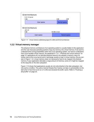
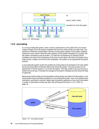
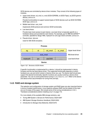
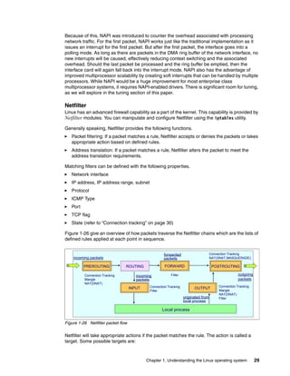
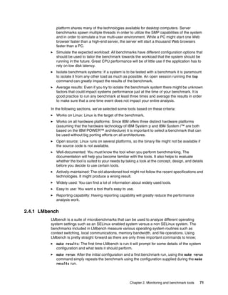
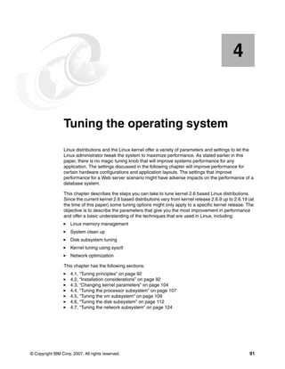
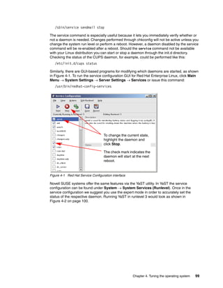
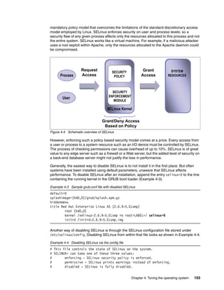
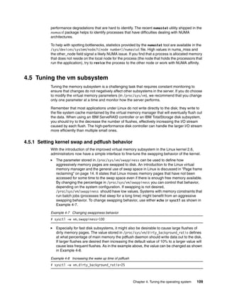
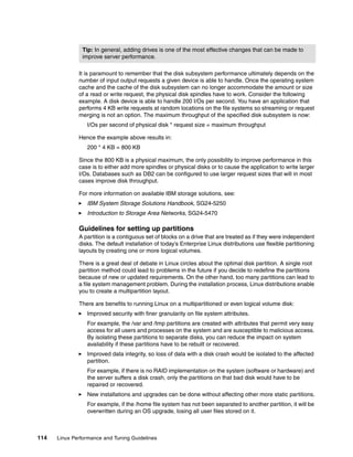
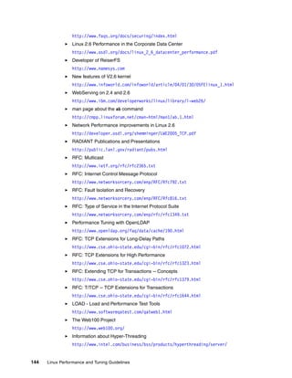
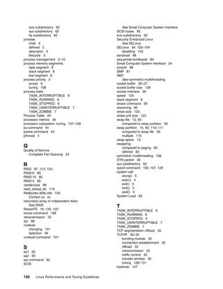
2.3.2 vmstat
vmstat provides information about processes, memory, paging, block I/O, traps, and CPU
activity. The vmstat command displays either average data or actual samples. The sampling
mode is enabled by providing vmstat with a sampling frequency and a sampling duration.
Example 2-2 Example output from vmstat
[root@lnxsu4 ~]# vmstat 2
procs -----------memory---------- ---swap-- -----io---- --system-- ----cpu----
r b swpd free buff cache si so bi bo in cs us sy id wa
0 1 0 1742264 112116 1999864 0 0 1 4 3 3 0 0 99 0
0 1 0 1742072 112208 1999772 0 0 0 2536 1258 1146 0 1 75 24
0 1 0 1741880 112260 1999720 0 0 0 2668 1235 1002 0 1 75 24
0 1 0 1741560 112308 1999932 0 0 0 2930 1240 1015 0 1 75 24
1 1 0 1741304 112344 2000416 0 0 0 2980 1238 925 0 1 75 24
0 1 0 1741176 112384 2000636 0 0 0 2968 1233 929 0 1 75 24
0 1 0 1741304 112420 2000600 0 0 0 3024 1247 925 0 1 75 24
Attention: In sampling mode consider the possibility of spikes between the actual data
collection. Changing sampling frequency to a lower value could evade such hidden spikes.
Note: The first data line of the vmstat report shows averages since the last reboot, so it
should be eliminated.

57. Chapter 2. Monitoring and benchmark tools 43
The columns in the output are as follows:
Process (procs) r: The number of processes waiting for runtime
b: The number of processes in uninterruptable sleep
Memory swpd: The amount of virtual memory used (KB)
free: The amount of idle memory (KB)
buff: The amount of memory used as buffers (KB)
cache: The amount of memory used as cache (KB)
Swap si: Amount of memory swapped from the disk (KBps)
so: Amount of memory swapped to the disk (KBps)
IO bi: Blocks sent to a block device (blocks/s)
bo: Blocks received from a block device (blocks/s)
System in: The number of interrupts per second, including the clock
cs: The number of context switches per second
CPU (% of total CPU time)
us: Time spent running non-kernel code (user time, including nice time).
sy: Time spent running kernel code (system time).
id: Time spent idle. Prior to Linux 2.5.41, this included I/O-wait time.
wa: Time spent waiting for IO. Prior to Linux 2.5.41, this appeared as
zero.
The vmstat command supports a vast number of command line parameters that are fully
documented in the man pages for vmstat. Some of the more useful flags include:
-m displays the memory utilization of the kernel (slabs)
-a provides information about active and inactive memory pages
-n displays only one header line, useful if running vmstat in sampling mode and
piping the output to a file. (For example, root#vmstat –n 2 10 generates vmstat
10 times with a sampling rate of two seconds.)
When used with the –p {partition} flag, vmstat also provides I/O statistics.
2.3.3 uptime
The uptime command can be used to see how long the server has been running and how
many users are logged on, as well as for a quick overview of the average load of the server.
(Refer to 1.6.1, “Processor metrics” on page 34). The system load average is displayed for
the past 1minute, 5 minute, and 15 minute intervals.
The optimal value of the load is 1, which means that each process has immediate access to
the CPU and there are no CPU cycles lost. The typical load can vary from system to system.
For a uniprocessor workstation, 1 or 2 might be acceptable, whereas you will probably see
values of 8 to 10 on multiprocessor servers.
You can use uptime to pinpoint a problem with your server or the network. For example, if a
network application is running poorly, run uptime and you will see whether the system load is
high. If not, the problem is more likely to be related to your network than to your server.
Tip: You can use w instead of uptime. w also provides information about who is currently
logged on to the machine and what the user is doing.

58. 44 Linux Performance and Tuning Guidelines
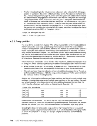
Example 2-3 Sample output of uptime
1:57am up 4 days 17:05, 2 users, load average: 0.00, 0.00, 0.00
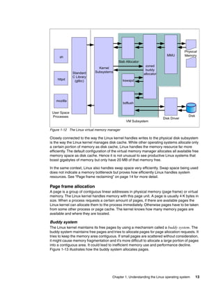
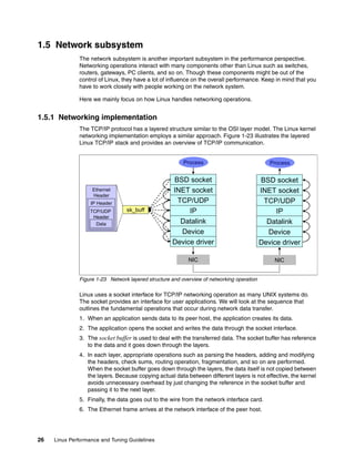
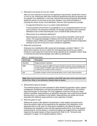
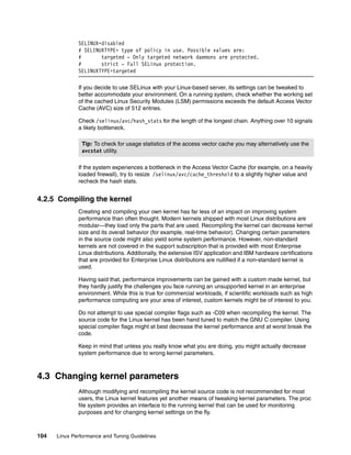
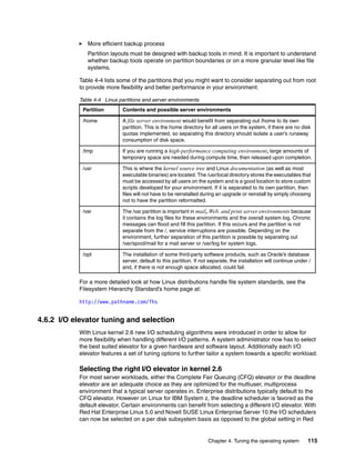
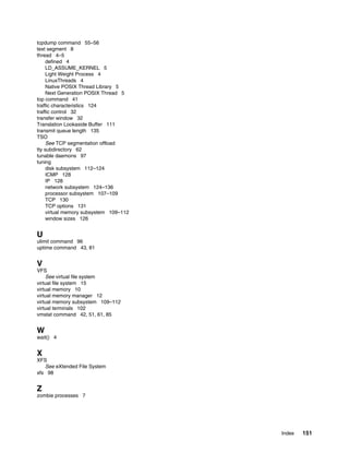
2.3.4 ps and pstree
The ps and pstree commands are some of the most basic commands when it comes to
system analysis. ps can have 3 different types of command options, UNIX style, BSD style
and GNU style. Here we look at UNIX style options.
The ps command provides a list of existing processes. The top command shows the process
information, but ps will provide more detailed information. The number of processes listed
depends on the options used. A simple ps -A command lists all processes with their
respective process ID (PID) that can be crucial for further investigation. A PID number is
required in order to use tools such as pmap or renice.
On systems running Java™ applications, the output of a ps -A command might easily fill up
the display to the point where it is difficult to get a complete picture of all running processes.
In this case, the pstree command might come in handy as it displays the running processes
in a tree structure and consolidates spawned subprocesses (for example, Java threads). The
pstree command can help identify originating processes. There is another ps variant, pgrep.
It might be useful as well.
Example 2-4 A sample ps output
[root@bc1srv7 ~]# ps -A
PID TTY TIME CMD
1 ? 00:00:00 init
2 ? 00:00:00 migration/0
3 ? 00:00:00 ksoftirqd/0
2347 ? 00:00:00 sshd
2435 ? 00:00:00 sendmail
27397 ? 00:00:00 sshd
27402 pts/0 00:00:00 bash
27434 pts/0 00:00:00 ps
We will look at some useful options for detailed information.
-e All processes. Identical to -A
-l Show long format
-F Extra full mode
-H Forest
-L Show threads, possibly with LWP and NLWP columns
-m Show threads after processes
Here’s an example of the detailed output of the processes using following command:
ps -elFL
Example 2-5 An example of detailed output
[root@lnxsu3 ~]# ps -elFL
F S UID PID PPID LWP C NLWP PRI NI ADDR SZ WCHAN RSS PSR STIME TTY TIME CMD
4 S root 1 0 1 0 1 76 0 - 457 - 552 0 Mar08 ? 00:00:01 init [3]
1 S root 2 1 2 0 1 -40 - - 0 migrat 0 0 Mar08 ? 00:00:36 [migration/0]
1 S root 3 1 3 0 1 94 19 - 0 ksofti 0 0 Mar08 ? 00:00:00 [ksoftirqd/0]

59. Chapter 2. Monitoring and benchmark tools 45
1 S root 4 1 4 0 1 -40 - - 0 migrat 0 1 Mar08 ? 00:00:27 [migration/1]
1 S root 5 1 5 0 1 94 19 - 0 ksofti 0 1 Mar08 ? 00:00:00 [ksoftirqd/1]
1 S root 6 1 6 0 1 -40 - - 0 migrat 0 2 Mar08 ? 00:00:00 [migration/2]
1 S root 7 1 7 0 1 94 19 - 0 ksofti 0 2 Mar08 ? 00:00:00 [ksoftirqd/2]
1 S root 8 1 8 0 1 -40 - - 0 migrat 0 3 Mar08 ? 00:00:00 [migration/3]
1 S root 9 1 9 0 1 94 19 - 0 ksofti 0 3 Mar08 ? 00:00:00 [ksoftirqd/3]
1 S root 10 1 10 0 1 65 -10 - 0 worker 0 0 Mar08 ? 00:00:00 [events/0]
1 S root 11 1 11 0 1 65 -10 - 0 worker 0 1 Mar08 ? 00:00:00 [events/1]
1 S root 12 1 12 0 1 65 -10 - 0 worker 0 2 Mar08 ? 00:00:00 [events/2]
1 S root 13 1 13 0 1 65 -10 - 0 worker 0 3 Mar08 ? 00:00:00 [events/3]
5 S root 3493 1 3493 0 1 76 0 - 1889 - 4504 1 Mar08 ? 00:07:40 hald
4 S root 3502 1 3502 0 1 78 0 - 374 - 408 1 Mar08 tty1 00:00:00 /sbin/mingetty tty1
4 S root 3503 1 3503 0 1 78 0 - 445 - 412 1 Mar08 tty2 00:00:00 /sbin/mingetty tty2
4 S root 3504 1 3504 0 1 78 0 - 815 - 412 2 Mar08 tty3 00:00:00 /sbin/mingetty tty3
4 S root 3505 1 3505 0 1 78 0 - 373 - 412 1 Mar08 tty4 00:00:00 /sbin/mingetty tty4
4 S root 3506 1 3506 0 1 78 0 - 569 - 412 3 Mar08 tty5 00:00:00 /sbin/mingetty tty5
4 S root 3507 1 3507 0 1 78 0 - 585 - 412 0 Mar08 tty6 00:00:00 /sbin/mingetty tty6
0 S takech 3509 1 3509 0 1 76 0 - 718 - 1080 0 Mar08 ? 00:00:00 /usr/libexec/gam_server
0 S takech 4057 1 4057 0 1 75 0 - 1443 - 1860 0 Mar08 ? 00:00:01 xscreensaver -nosplash
4 S root 4239 1 4239 0 1 75 0 - 5843 - 9180 1 Mar08 ? 00:00:01 /usr/bin/metacity
--sm-client-id=default1
0 S takech 4238 1 4238 0 1 76 0 - 3414 - 5212 2 Mar08 ? 00:00:00 /usr/bin/metacity
--sm-client-id=default1
4 S root 4246 1 4246 0 1 76 0 - 5967 - 12112 2 Mar08 ? 00:00:00 gnome-panel
--sm-client-id default2
0 S takech 4247 1 4247 0 1 77 0 - 5515 - 11068 0 Mar08 ? 00:00:00 gnome-panel
--sm-client-id default2
0 S takech 4249 1 4249 0 9 76 0 - 10598 - 17520 1 Mar08 ? 00:00:01 nautilus
--no-default-window --sm-client-id default3
1 S takech 4249 1 4282 0 9 75 0 - 10598 - 17520 0 Mar08 ? 00:00:00 nautilus
--no-default-window --sm-client-id default3
1 S takech 4249 1 4311 0 9 75 0 - 10598 322565 17520 0 Mar08 ? 00:00:00 nautilus
--no-default-window --sm-client-id default3
1 S takech 4249 1 4312 0 9 75 0 - 10598 322565 17520 0 Mar08 ? 00:00:00 nautilus
--no-default-window --sm-client-id default3
The columns in the output are:
F Process flag
S State of the process: S=sleeping, R=running, T=stopped or traced,
D=interruptable sleep, Z=zombie. The process state is discussed further in 1.1.7,
“Process state” on page 6.
UID Name of the user who owns (and perhaps started) the process.
PID Process ID number
PPID Parent process ID number
LWP LWP(light weight process, or thread) ID of the lwp being reported.
C Integer value of the processor utilization percentage.(CPU usage)
NLWP Number of lwps (threads) in the process. (alias thcount).
PRI Priority of the process. (See 1.1.4, “Process priority and nice level” on page 5 for
details.)
NI Niceness level (whether the process tries to be nice by adjusting the priority by
the number given; see below for details).
ADDR Process Address space (not displayed)
SZ Amount of memory (code+data+stack) used by the process in kilobytes.

60. 46 Linux Performance and Tuning Guidelines
WCHAN Name of the kernel function in which the process is sleeping, a “-” if the process is
running, or a “*” if the process is multi-threaded and ps is not displaying threads.
RSS Resident set size, the non-swapped physical memory that a task has used (in
kiloBytes).
PSR Processor that process is currently assigned to.
STIME Time the command started.
TTY Terminal
TIME Total CPU time used by the process (since it was started).
CMD Command line used to start the task (including parameters).
Thread information
You can see the thread information using ps -L option.
Example 2-6 thread information with ps -L
[root@edam ~]# ps -eLF| grep -E "LWP|/usr/sbin/httpd"
UID PID PPID LWP C NLWP SZ RSS PSR STIME TTY TIME CMD
root 4504 1 4504 0 1 4313 8600 2 08:33 ? 00:00:00 /usr/sbin/httpd
apache 4507 4504 4507 0 1 4313 4236 1 08:33 ? 00:00:00 /usr/sbin/httpd
apache 4508 4504 4508 0 1 4313 4228 1 08:33 ? 00:00:00 /usr/sbin/httpd
apache 4509 4504 4509 0 1 4313 4228 0 08:33 ? 00:00:00 /usr/sbin/httpd
apache 4510 4504 4510 0 1 4313 4228 3 08:33 ? 00:00:00 /usr/sbin/httpd
[root@edam ~]# ps -eLF| grep -E "LWP|/usr/sbin/httpd"
UID PID PPID LWP C NLWP SZ RSS PSR STIME TTY TIME CMD
root 4632 1 4632 0 1 3640 7772 2 08:44 ? 00:00:00 /usr/sbin/httpd.worker
apache 4635 4632 4635 0 27 72795 5352 3 08:44 ? 00:00:00 /usr/sbin/httpd.worker
apache 4635 4632 4638 0 27 72795 5352 1 08:44 ? 00:00:00 /usr/sbin/httpd.worker
apache 4635 4632 4639 0 27 72795 5352 3 08:44 ? 00:00:00 /usr/sbin/httpd.worker
apache 4635 4632 4640 0 27 72795 5352 3 08:44 ? 00:00:00 /usr/sbin/httpd.worker
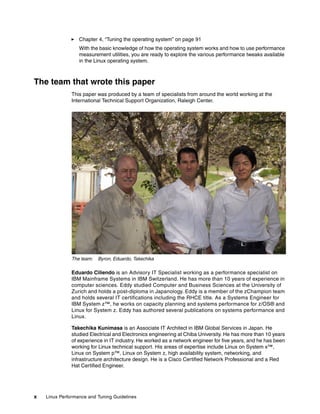
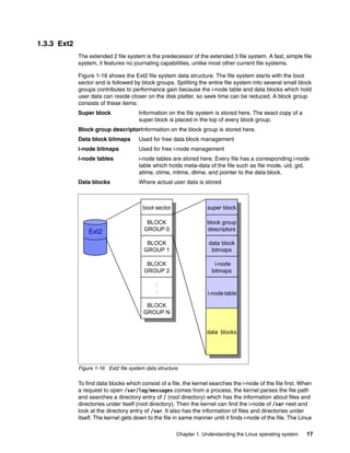
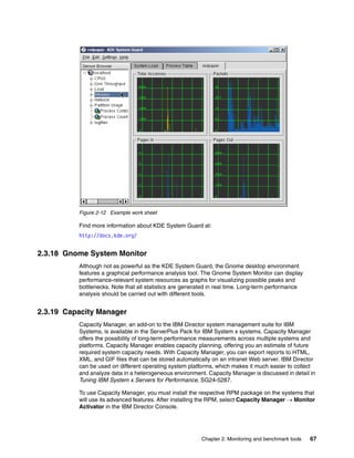
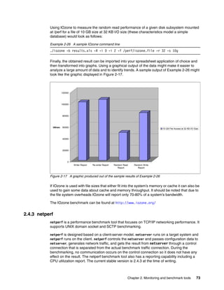
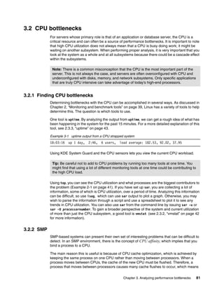
2.3.5 free
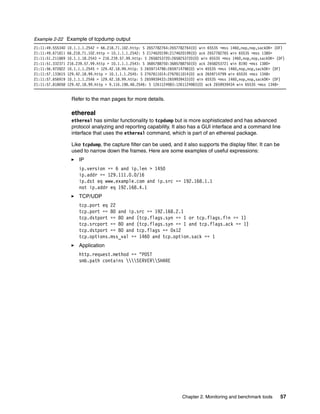
The command /bin/free displays information about the total amount of free and used
memory (including swap) on the system. It also includes information about the buffers and
cache used by the kernel.
Example 2-7 Example output from the free command
total used free shared buffers cached
Mem: 1291980 998940 293040 0 89356 772016
-/+ buffers/cache: 137568 1154412
Swap: 2040244 0 2040244
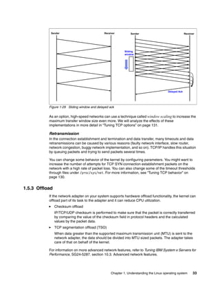
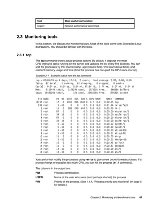
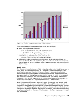
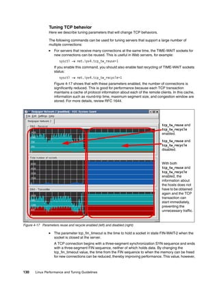
When using free, remember the Linux memory architecture and the way the virtual memory
manager works. The amount of free memory is of limited use, and the pure utilization
statistics of swap are not an indication of a memory bottleneck.
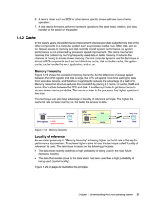
Figure 2-1 on page 47 depicts the basic idea of what free command output shows.

61. Chapter 2. Monitoring and benchmark tools 47
Figure 2-1 free command output
Useful parameters for the free command include:
-b, -k, -m, -g Display values in bytes, kilobytes, megabytes, and gigabytes
-l Distinguishes between low and high memory (Refer to 1.2, “Linux memory
architecture” on page 10.)
-c <count> Displays the free output <count> number of times
Memory used in a zone
Using the -l option, you can see how much memory is used in each memory zone.
Example 2-8 and Example 2-9 show the example of free -l output of 32 bit and 64 bit
systems. Notice that 64-bit systems no longer use high memory.
Example 2-8 Example output from the free command on 32 bit version kernel
[root@edam ~]# free -l
total used free shared buffers cached
Mem: 4154484 2381500 1772984 0 108256 1974344
Low: 877828 199436 678392
High: 3276656 2182064 1094592
-/+ buffers/cache: 298900 3855584
Swap: 4194296 0 4194296
Example 2-9 Example output from the free command on 64 bit version kernel
[root@lnxsu4 ~]# free -l
total used free shared buffers cached
Mem: 4037420 138508 3898912 0 10300 42060
Low: 4037420 138508 3898912
High: 0 0 0
-/+ buffers/cache: 86148 3951272
#free -m
total used free shared buffers cached
Mem: 4092 3270 826 0 36 1482
-/+ buffers/cache: 1748 2344
Swap: 4096 0 4096
free
memory
(KB)
used
memory
(KB)
shared
memory
(KB)
buffer
(KB)
cache
(KB)
Free= 826(MB)
Buffer=36(MB)
Cache=1482(MB)
Used=1748(MB)
memory 4GB
Free= 826(MB)
Buffer=36(MB)
Cache=1482(MB)
Used=1748(MB)
memory 4GB
total amount
of memory
(KB)
Mem : used = Used + Buffer + Cache / free = Free
-/+ buffers/cache : used = Used / free = Free + Buffer + Cache

62. 48 Linux Performance and Tuning Guidelines
Swap: 2031608 332 2031276
You can also determine how many chunks of memory are available in each zone using
/proc/buddyinfo file. Each column of numbers means the number of pages of that order
which are available. In Example 2-10, there are 5 chunks of 2^2*PAGE_SIZE available in
ZONE_DMA, and 16 chunks of 2^3*PAGE_SIZE available in ZONE_DMA32. Remember how
the buddy system allocates pages (refer to “Buddy system” on page 13). This information
shows you how fragmented the memory is and gives you an idea of how many pages you can
safely allocate.
Example 2-10 Buddy system information for 64 bit system
[root@lnxsu5 ~]# cat /proc/buddyinfo
Node 0, zone DMA 1 3 5 4 6 1 1 0 2 0 2
Node 0, zone DMA32 56 14 2 16 7 3 1 7 41 42 670
Node 0, zone Normal 0 6 3 2 1 0 1 0 0 1 0
2.3.6 iostat
The iostat command shows average CPU times since the system was started (similar to
uptime). It also creates a report of the activities of the disk subsystem of the server in two
parts: CPU utilization and device (disk) utilization. To use iostat to perform detailed I/O
bottleneck and performance tuning, see 3.4.1, “Finding disk bottlenecks” on page 84. The
iostat utility is part of the sysstat package.
Example 2-11 Sample output of iostat
Linux 2.4.21-9.0.3.EL (x232) 05/11/2004
avg-cpu: %user %nice %sys %idle
0.03 0.00 0.02 99.95
Device: tps Blk_read/s Blk_wrtn/s Blk_read Blk_wrtn
dev2-0 0.00 0.00 0.04 203 2880
dev8-0 0.45 2.18 2.21 166464 168268
dev8-1 0.00 0.00 0.00 16 0
dev8-2 0.00 0.00 0.00 8 0
dev8-3 0.00 0.00 0.00 344 0
The CPU utilization report has four sections:
%user Shows the percentage of CPU utilization that was taken up while executing at
the user level (applications).
%nice Shows the percentage of CPU utilization that was taken up while executing at
the user level with a nice priority. (Priority and nice levels are described in
2.3.7, “nice, renice” on page 67.)
%sys Shows the percentage of CPU utilization that was taken up while executing at
the system level (kernel).
%idle Shows the percentage of time the CPU was idle.
The device utilization report has these sections:
Device The name of the block device.

63. Chapter 2. Monitoring and benchmark tools 49
tps The number of transfers per second (I/O requests per second) to the device.
Multiple single I/O requests can be combined in a transfer request, because
a transfer request can have different sizes.
Blk_read/s, Blk_wrtn/s
Blocks read and written per second indicate data read from or written to the
device in seconds. Blocks can also have different sizes. Typical sizes are
1024, 2048, and 4048 bytes, depending on the partition size. For example,
the block size of /dev/sda1 can be found with:
dumpe2fs -h /dev/sda1 |grep -F "Block size"
This produces output similar to:
dumpe2fs 1.34 (25-Jul-2003)
Block size: 1024
Blk_read, Blk_wrtn
Indicates the total number of blocks read and written since the boot.
The iostat can use many options. The most useful one is -x option from the performance
perspective. It displays extended statistics. The following is sample output.
Example 2-12 iostat -x extended statistics display
[root@lnxsu4 ~]# iostat -d -x sdb 1
Linux 2.6.9-42.ELsmp (lnxsu4.itso.ral.ibm.com) 03/18/2007
Device: rrqm/s wrqm/s r/s w/s rsec/s wsec/s rkB/s wkB/s avgrq-sz avgqu-sz await svctm %util
sdb 0.15 0.00 0.02 0.00 0.46 0.00 0.23 0.00 29.02 0.00 2.60 1.05 0.00
rrqm/s, wrqm/s
The number of read/write requests merged per second that were issued to
the device. Multiple single I/O requests can be merged in a transfer request,
because a transfer request can have different sizes.
r/s, w/s The number of read/write requests that were issued to the device per
second.
rsec/s, wsec/s The number of sectors read/write from the device per second.
rkB/s, wkB/s The number of kilobytes read/write from the device per second.
avgrq-sz The average size of the requests that were issued to the device. This value is
is displayed in sectors.
avgqu-sz The average queue length of the requests that were issued to the device.
await Shows the percentage of CPU utilization that was used while executing at the
system level (kernel).
svctm The average service time (in milliseconds) for I/O requests that were issued
to the device.
%util Percentage of CPU time during which I/O requests were issued to the device
(bandwidth utilization for the device). Device saturation occurs when this
value is close to 100%.
It might be useful to calculate the average I/O size in order to tailor a disk subsystem towards
the access pattern. The following example is the output of using iostat with the -d and -x
flag in order to display only information about the disk subsystem of interest:

64. 50 Linux Performance and Tuning Guidelines
Example 2-13 Using iostat -x -d to analyze the average I/O size
Device: rrqm/s wrqm/s r/s w/s rsec/s wsec/s rkB/s wkB/s avgrq-sz avgqu-sz await svctm %util
dasdc 0.00 0.00 0.00 2502.97 0.00 24601.98 0.00 12300.99 9.83 142.93 57.08 0.40 100.00
The iostat output in Example 2-13 shows that the device dasdc had to write 12300.99 KB of
data per second as being displayed under the kB_wrtn/s heading. This amount of data was
being sent to the disk subsystem in 2502.97 I/Os as shown under w/s in the example above.
The average I/O size or average request size is displayed under avgrq-sz and is 9.83 blocks
of 512 byte in our example. For async writes the average I/O size is usually some odd
number. However most applications perform read and write I/O in multiples of 4 KB (for
instance 4 KB, 8 KB, 16 KB, 32 KB, and so on). In the example above the application was
issuing nothing but random write requests of 4 KB, however iostat shows an average request
size of 4.915 KB. The difference is caused by the Linux file system that, even though we were
performing random writes, found some I/Os that could be merged together for more efficient
flushing out to the disk subsystem.
2.3.7 sar
The sar command is used to collect, report, and save system activity information. The sar
command consists of three applications: sar, which displays the data, and sa1 and sa2, which
are used for collecting and storing the data. The sar tool features a wide range of options so
be sure to check the man page for it. The sar utility is part of the sysstat package.
With sa1 and sa2, the system can be configured to get information and log it for later analysis.
To accomplish this, add the lines to /etc/crontab (Example 2-14). Keep in mind that a default
cron job running sar daily is set up automatically after installing sar on your system.
Example 2-14 Example of starting automatic log reporting with cron
# 8am-7pm activity reports every 10 minutes during weekdays.
*/10 8-18 * * 1-5 /usr/lib/sa/sa1 600 6 &
# 7pm-8am activity reports every an hour during weekdays.
0 19-7 * * 1-5 /usr/lib/sa/sa1 &
# Activity reports every an hour on Saturday and Sunday.
0 * * * 0,6 /usr/lib/sa/sa1 &
# Daily summary prepared at 19:05
5 19 * * * /usr/lib/sa/sa2 -A &
The raw data for the sar tool is stored under /var/log/sa/ where the various files represent the
days of the respective month. To examine your results, select the weekday of the month and
the requested performance data. For example, to display the network counters from the 21st,
use the command sar -n DEV -f sa21 and pipe it to less as in Example 2-15 on page 51.
Note: When using the default async mode for file systems, only the average request size
displayed in iostat is correct. Even though applications perform write requests at distinct
sizes, the I/O layer of Linux will most likely merge and hence alter the average I/O size.
Tip: We suggest that you have sar running on most if not all of your systems. In case of a
performance problem, you will have very detailed information on hand at very small
overhead and no additional cost.

65. Chapter 2. Monitoring and benchmark tools 51
Example 2-15 Displaying system statistics with sar
[root@linux sa]# sar -n DEV -f sa21 | less
Linux 2.6.9-5.ELsmp (linux.itso.ral.ibm.com) 04/21/2005
12:00:01 AM IFACE rxpck/s txpck/s rxbyt/s txbyt/s rxcmp/s txcmp/s rxmcst/s
12:10:01 AM lo 0.00 0.00 0.00 0.00 0.00 0.00 0.00
12:10:01 AM eth0 1.80 0.00 247.89 0.00 0.00 0.00 0.00
12:10:01 AM eth1 0.00 0.00 0.00 0.00 0.00 0.00 0.00
You can also use sar to run near-real-time reporting from the command line (Example 2-16).
Example 2-16 Ad hoc CPU monitoring
[root@x232 root]# sar -u 3 10
Linux 2.4.21-9.0.3.EL (x232) 05/22/2004
02:10:40 PM CPU %user %nice %system %idle
02:10:43 PM all 0.00 0.00 0.00 100.00
02:10:46 PM all 0.33 0.00 0.00 99.67
02:10:49 PM all 0.00 0.00 0.00 100.00
02:10:52 PM all 7.14 0.00 18.57 74.29
02:10:55 PM all 71.43 0.00 28.57 0.00
02:10:58 PM all 0.00 0.00 100.00 0.00
02:11:01 PM all 0.00 0.00 0.00 0.00
02:11:04 PM all 0.00 0.00 100.00 0.00
02:11:07 PM all 50.00 0.00 50.00 0.00
02:11:10 PM all 0.00 0.00 100.00 0.00
Average: all 1.62 0.00 3.33 95.06
From the collected data, you see a detailed overview of CPU utilization (%user, %nice,
%system, %idle), memory paging, network I/O and transfer statistics, process creation
activity, activity for block devices, and interrupts/second over time.
2.3.8 mpstat
The mpstat command is used to report the activities of each of the available CPUs on a
multiprocessor server. Global average activities among all CPUs are also reported. The
mpstat utility is part of the sysstat package.
The mpstat utility enables you to display overall CPU statistics per system or per processor.
mpstat also enables the creation of statistics when used in sampling mode analogous to the
vmstat command with a sampling frequency and a sampling count. Example 2-17 shows a
sample output created with mpstat -P ALL to display average CPU utilization per processor.
Example 2-17 Output of mpstat command on multiprocessor system
[root@linux ~]# mpstat -P ALL
Linux 2.6.9-5.ELsmp (linux.itso.ral.ibm.com) 04/22/2005
03:19:21 PM CPU %user %nice %system %iowait %irq %soft %idle intr/s
03:19:21 PM all 0.03 0.00 0.34 0.06 0.02 0.08 99.47 1124.22
03:19:21 PM 0 0.03 0.00 0.33 0.03 0.04 0.15 99.43 612.12
03:19:21 PM 1 0.03 0.00 0.36 0.10 0.01 0.01 99.51 512.09

66. 52 Linux Performance and Tuning Guidelines
To display three entries of statistics for all processors of a multiprocessor server at
one-second intervals, use the command:
mpstat -P ALL 1 2
Example 2-18 Output of mpstat command on two-way machine
[root@linux ~]# mpstat -P ALL 1 2
Linux 2.6.9-5.ELsmp (linux.itso.ral.ibm.com) 04/22/2005
03:31:51 PM CPU %user %nice %system %iowait %irq %soft %idle intr/s
03:31:52 PM all 0.00 0.00 0.00 0.00 0.00 0.00 100.00 1018.81
03:31:52 PM 0 0.00 0.00 0.00 0.00 0.00 0.00 100.00 991.09
03:31:52 PM 1 0.00 0.00 0.00 0.00 0.00 0.00 99.01 27.72
Average: CPU %user %nice %system %iowait %irq %soft %idle intr/s
Average: all 0.00 0.00 0.00 0.00 0.00 0.00 100.00 1031.89
Average: 0 0.00 0.00 0.00 0.00 0.00 0.00 100.00 795.68
Average: 1 0.00 0.00 0.00 0.00 0.00 0.00 99.67 236.54
For the complete syntax of the mpstat command, issue:
mpstat -?
2.3.9 numastat
With Non-Uniform Memory Architecture (NUMA) systems such as the IBM System x 3950,
NUMA architectures have become mainstream in enterprise data centers. However, NUMA
systems introduce new challenges to the performance tuning process. Topics such as
memory locality were of no interest until NUMA systems arrived. Luckily, Enterprise Linux
distributions provide a tool for monitoring the behavior of NUMA architectures. The numastat
command provides information about the ratio of local versus remote memory usage and the
overall memory configuration of all nodes. Failed allocations of local memory, as displayed in
the numa_miss column and allocations of remote memory (slower memory), as displayed in
the numa_foreign column should be investigated. Excessive allocation of remote memory will
increase system latency and likely decrease overall performance. Binding processes to a
node with the memory map in the local RAM will most likely improve performance.
Example 2-19 Sample output of the numastat command
[root@linux ~]# numastat
node1 node0
numa_hit 76557759 92126519
numa_miss 30772308 30827638
numa_foreign 30827638 30772308
interleave_hit 106507 103832
local_node 76502227 92086995
other_node 30827840 30867162
2.3.10 pmap
The pmap command reports the amount of memory that one or more processes are using. You
can use this tool to determine which processes on the server are being allocated memory and

67. Chapter 2. Monitoring and benchmark tools 53
whether this amount of memory is a cause of memory bottlenecks. For detailed information,
use pmap -d option.
pmap -d <pid>
Example 2-20 Process memory information the init process is using
[root@lnxsu4 ~]# pmap -d 1
1: init [3]
Address Kbytes Mode Offset Device Mapping
0000000000400000 36 r-x-- 0000000000000000 0fd:00000 init
0000000000508000 8 rw--- 0000000000008000 0fd:00000 init
000000000050a000 132 rwx-- 000000000050a000 000:00000 [ anon ]
0000002a95556000 4 rw--- 0000002a95556000 000:00000 [ anon ]
0000002a95574000 8 rw--- 0000002a95574000 000:00000 [ anon ]
00000030c3000000 84 r-x-- 0000000000000000 0fd:00000 ld-2.3.4.so
00000030c3114000 8 rw--- 0000000000014000 0fd:00000 ld-2.3.4.so
00000030c3200000 1196 r-x-- 0000000000000000 0fd:00000 libc-2.3.4.so
00000030c332b000 1024 ----- 000000000012b000 0fd:00000 libc-2.3.4.so
00000030c342b000 8 r---- 000000000012b000 0fd:00000 libc-2.3.4.so
00000030c342d000 12 rw--- 000000000012d000 0fd:00000 libc-2.3.4.so
00000030c3430000 16 rw--- 00000030c3430000 000:00000 [ anon ]
00000030c3700000 56 r-x-- 0000000000000000 0fd:00000 libsepol.so.1
00000030c370e000 1020 ----- 000000000000e000 0fd:00000 libsepol.so.1
00000030c380d000 4 rw--- 000000000000d000 0fd:00000 libsepol.so.1
00000030c380e000 32 rw--- 00000030c380e000 000:00000 [ anon ]
00000030c4500000 56 r-x-- 0000000000000000 0fd:00000 libselinux.so.1
00000030c450e000 1024 ----- 000000000000e000 0fd:00000 libselinux.so.1
00000030c460e000 4 rw--- 000000000000e000 0fd:00000 libselinux.so.1
00000030c460f000 4 rw--- 00000030c460f000 000:00000 [ anon ]
0000007fbfffc000 16 rw--- 0000007fbfffc000 000:00000 [ stack ]
ffffffffff600000 8192 ----- 0000000000000000 000:00000 [ anon ]
mapped: 12944K writeable/private: 248K shared: 0K
Some of the most important information is at the bottom of the display. The line shows:
mapped: total amount of memory mapped to files used in the process
writable/private: the amount of private address space this process is taking
shared: the amount of address space this process is sharing with others
You can also look at the address spaces where the information is stored. You can find an
interesting difference when you issue the pmap command on 32-bit and 64-bit systems. For
the complete syntax of the pmap command, issue:
pmap -?
2.3.11 netstat
netstat is one of the most popular tools. If you work on the network. you should be familiar
with this tool. It displays a lot of network related information such as socket usage, routing,
interface, protocol, network statistics, and more. Here are some of the basic options:
-a Show all socket information
-r Show routing information
-i Show network interface statistics
-s Show network protocol statistics

68. 54 Linux Performance and Tuning Guidelines
There are many other useful options. Please check man page. The following example
displays sample output of socket information.
Example 2-21 Showing socket information with netstat
[root@lnxsu5 ~]# netstat -natuw
Active Internet connections (servers and established)
Proto Recv-Q Send-Q Local Address Foreign Address State
tcp 0 0 0.0.0.0:111 0.0.0.0:* LISTEN
tcp 0 0 127.0.0.1:25 0.0.0.0:* LISTEN
tcp 0 0 127.0.0.1:2207 0.0.0.0:* LISTEN
tcp 0 0 127.0.0.1:36285 127.0.0.1:12865 TIME_WAIT
tcp 0 0 10.0.0.5:37322 10.0.0.4:33932 TIME_WAIT
tcp 0 1 10.0.0.5:55351 10.0.0.4:33932 SYN_SENT
tcp 0 1 10.0.0.5:55350 10.0.0.4:33932 LAST_ACK
tcp 0 0 10.0.0.5:64093 10.0.0.4:33932 TIME_WAIT
tcp 0 0 10.0.0.5:35122 10.0.0.4:12865 ESTABLISHED
tcp 0 0 10.0.0.5:17318 10.0.0.4:33932 TIME_WAIT
tcp 0 0 :::22 :::* LISTEN
tcp 0 2056 ::ffff:192.168.0.254:22 ::ffff:192.168.0.1:3020 ESTABLISHED
udp 0 0 0.0.0.0:111 0.0.0.0:*
udp 0 0 0.0.0.0:631 0.0.0.0:*
udp 0 0 :::5353 :::*
Socket information
Proto The protocol (tcp, udp, raw) used by the socket.
Recv-Q The count of bytes not copied by the user program connected to this
socket.
Send-Q The count of bytes not acknowledged by the remote host.
Local Address Address and port number of the local end of the socket. Unless the
--numeric (-n) option is specified, the socket address is resolved to its
canonical host name (FQDN), and the port number is translated into the
corresponding service name.
Foreign Address Address and port number of the remote end of the socket.
State The state of the socket. Since there are no states in raw mode and
usually no states used in UDP, this column may be left blank. For possible
states, see Figure 1-28 on page 32 and man page.
2.3.12 iptraf
iptraf monitors TCP/IP traffic in a real time manner and generates real time reports. It shows
TCP/IP traffic statistics by each session, by interface, and by protocol. The iptraf utility is
provided by the iptraf package.
The iptraf give us reports like the following:
򐂰 IP traffic monitor: Network traffic statistics by TCP connection
򐂰 General interface statistics: IP traffic statistics by network interface
򐂰 Detailed interface statistics: Network traffic statistics by protocol
򐂰 Statistical breakdowns: Network traffic statistics by TCP/UDP port and by packet size
򐂰 LAN station monitor: Network traffic statistics by Layer2 address
Following are a few of the reports iptraf generates.

69. Chapter 2. Monitoring and benchmark tools 55
Figure 2-2 iptraf output of TCP/IP statistics by protocol
Figure 2-3 iptraf output of TCP/IP traffic statistics by packet size
2.3.13 tcpdump / ethereal
The tcpdump and ethereal are used to capture and analyze network traffic. Both tool use the
libpcap library to capture packets. They monitor all the traffic on a network adapter with
promiscuous mode and capture all the frames the adapter has received. To capture all the
packets, these commands should be executed with super user privilege to make the interface
promiscuous mode.

70. 56 Linux Performance and Tuning Guidelines
You can use these tools to dig into the network related problems. You can find TCP/IP
retransmission, windows size scaling, name resolution problem, network misconfiguration,
and more. Just keep in mind that these tools can monitor only frames the network adapter
has received, not entire network traffic.
tcpdump
tcpdump is a simple but robust utility. It has basic protocol analyzing capability allowing you to
get a rough picture of what is happening on the network. tcpdump supports many options and
flexible expressions for filtering the frames to be captured (capture filter). We’ll take a look at
this below.
Options:
-i <interface> Network interface
-e Print the link-level header
-s <snaplen> Capture <snaplen> bytes from each packet
-n Avoide DNS lookup
-w <file> Write to file
-r <file> Read from file
-v, -vv, -vvv Vervose output
Expressions for the capture filter:
Keywords:
host dst, src, port, src port, dst port, tcp, udp, icmp, net, dst net, src net, and more
Primitives may be combined using:
Negation (‘`!‘ or ‘not‘)
Concatenation (`&&' or `and')
Alternation (`||' or `or')
Example of some useful expressions:
򐂰 DNS query packets
tcpdump -i eth0 'udp port 53'
򐂰 FTP control and FTP data session to 192.168.1.10
tcpdump -i eth0 'dst 192.168.1.10 and (port ftp or ftp-data)'
򐂰 HTTP session to 192.168.2.253
tcpdump -ni eth0 'dst 192.168.2.253 and tcp and port 80'
򐂰 Telnet session to subnet 192.168.2.0/24
tcpdump -ni eth0 'dst net 192.168.2.0/24 and tcp and port 22'
򐂰 Packets for which the source and destination are not in subnet 192.168.1.0/24 with TCP
SYN or TCP FIN flags on (TCP establishment or termination)
tcpdump 'tcp[tcpflags] & (tcp-syn|tcp-fin) != 0 and not src and dst net
192.168.1.0/24'

71. Chapter 2. Monitoring and benchmark tools 57
Example 2-22 Example of tcpdump output
21:11:49.555340 10.1.1.1.2542 > 66.218.71.102.http: S 2657782764:2657782764(0) win 65535 <mss 1460,nop,nop,sackOK> (DF)
21:11:49.671811 66.218.71.102.http > 10.1.1.1.2542: S 2174620199:2174620199(0) ack 2657782765 win 65535 <mss 1380>
21:11:51.211869 10.1.1.18.2543 > 216.239.57.99.http: S 2658253720:2658253720(0) win 65535 <mss 1460,nop,nop,sackOK> (DF)
21:11:51.332371 216.239.57.99.http > 10.1.1.1.2543: S 3685788750:3685788750(0) ack 2658253721 win 8190 <mss 1380>
21:11:56.972822 10.1.1.1.2545 > 129.42.18.99.http: S 2659714798:2659714798(0) win 65535 <mss 1460,nop,nop,sackOK> (DF)
21:11:57.133615 129.42.18.99.http > 10.1.1.1.2545: S 2767811014:2767811014(0) ack 2659714799 win 65535 <mss 1348>
21:11:57.656919 10.1.1.1.2546 > 129.42.18.99.http: S 2659939433:2659939433(0) win 65535 <mss 1460,nop,nop,sackOK> (DF)
21:11:57.818058 129.42.18.99.http > 9.116.198.48.2546: S 1261124983:1261124983(0) ack 2659939434 win 65535 <mss 1348>
Refer to the man pages for more details.
ethereal
ethereal has similar functionality to tcpdump but is more sophisticated and has advanced
protocol analyzing and reporting capability. It also has a GUI interface and a command line
interface that uses the ethereal command, which is part of an ethereal package.
Like tcpdump, the capture filter can be used, and it also supports the display filter. It can be
used to narrow down the frames. Here are some examples of useful expressions:
򐂰 IP
ip.version == 6 and ip.len > 1450
ip.addr == 129.111.0.0/16
ip.dst eq www.example.com and ip.src == 192.168.1.1
not ip.addr eq 192.168.4.1
򐂰 TCP/UDP
tcp.port eq 22
tcp.port == 80 and ip.src == 192.168.2.1
tcp.dstport == 80 and (tcp.flags.syn == 1 or tcp.flags.fin == 1)
tcp.srcport == 80 and (tcp.flags.syn == 1 and tcp.flags.ack == 1)
tcp.dstport == 80 and tcp.flags == 0x12
tcp.options.mss_val == 1460 and tcp.option.sack == 1
򐂰 Application
http.request.method == "POST
smb.path contains SERVERSHARE

72. 58 Linux Performance and Tuning Guidelines
Figure 2-4 ethereal GUI
2.3.14 nmon
nmon, short for Nigel's Monitor, is a popular tool to monitor Linux systems performance
developed by Nigel Griffiths. Since nmon incorporates the performance information for
several subsystems, it can be used as a single source for performance monitoring. Some of
the tasks that can be achieved with nmon include processor utilization, memory utilization,
run queue information, disks I/O statistics, network I/O statistics, paging activity, and process
metrics.
In order to run nmon, simply start the tool and select the subsystems of interest by typing their
one-key commands. For example, to get CPU, memory, and disk statistics, start nmon and
type c m d.
A very useful feature of nmon is the ability to save performance statistics for later analysis in a
comma separated values (CSV) file. The CSV output of nmon can be imported into a
spreadsheet application in order to produce graphical reports. In order to do so nmon should
be started with the -f flag (see nmon -h for the details). For example running nmon for an
hour capturing data snapshots every 30 seconds would be achieved using the command in
Example 2-23 on page 59.

73. Chapter 2. Monitoring and benchmark tools 59
Example 2-23 Using nmon to record performance data
# nmon -f -s 30 -c 120
The output of the above command will be stored in a text file in the current directory named
<hostname>_date_time.nmon.
For more information on nmon we suggest you visit
http://www-941.haw.ibm.com/collaboration/wiki/display/WikiPtype/nmon
In order to download nmon, visit
http://www.ibm.com/collaboration/wiki/display/WikiPtype/nmonanalyser
2.3.15 strace
The strace command intercepts and records the system calls that are called by a process,
and the signals that are received by a process. This is a useful diagnostic, instructional, and
debugging tool. System administrators find it valuable for solving problems with programs.
To trace a process, specify the process ID (PID) to be monitored:
strace -p <pid>
Example 2-24 shows an example of the output of strace.
Example 2-24 Output of strace monitoring httpd process
[root@x232 html]# strace -p 815
Process 815 attached - interrupt to quit
semop(360449, 0xb73146b8, 1) = 0
poll([{fd=4, events=POLLIN}, {fd=3, events=POLLIN, revents=POLLIN}], 2, -1) = 1
accept(3, {sa_family=AF_INET, sin_port=htons(52534), sin_addr=inet_addr("192.168.1.1")}, [16]) = 13
semop(360449, 0xb73146be, 1) = 0
getsockname(13, {sa_family=AF_INET, sin_port=htons(80), sin_addr=inet_addr("192.168.1.2")}, [16]) = 0
fcntl64(13, F_GETFL) = 0x2 (flags O_RDWR)
fcntl64(13, F_SETFL, O_RDWR|O_NONBLOCK) = 0
read(13, 0x8259bc8, 8000) = -1 EAGAIN (Resource temporarily unavailable)
poll([{fd=13, events=POLLIN, revents=POLLIN}], 1, 300000) = 1
read(13, "GET /index.html HTTP/1.0rnUser-A"..., 8000) = 91
gettimeofday({1084564126, 750439}, NULL) = 0
stat64("/var/www/html/index.html", {st_mode=S_IFREG|0644, st_size=152, ...}) = 0
open("/var/www/html/index.html", O_RDONLY) = 14
mmap2(NULL, 152, PROT_READ, MAP_SHARED, 14, 0) = 0xb7052000
writev(13, [{"HTTP/1.1 200 OKrnDate: Fri, 14 M"..., 264}, {"<html>n<title>n RedPaper Per"...,
152}], 2) = 416
munmap(0xb7052000, 152) = 0
socket(PF_UNIX, SOCK_STREAM, 0) = 15
connect(15, {sa_family=AF_UNIX, path="/var/run/.nscd_socket"}, 110) = -1 ENOENT (No such file or directory)
close(15) = 0
Here’s another interesting use. This command reports how much time has been consumed in
the kernel by each system call to execute a command.
strace -c <command>
Attention: While the strace command is running against a process, the performance of
the PID is drastically reduced and should only be run for the time of data collection.

74. 60 Linux Performance and Tuning Guidelines
Example 2-25 Output of strace counting for system time
[root@lnxsu4 ~]# strace -c find /etc -name httpd.conf
/etc/httpd/conf/httpd.conf
Process 3563 detached
% time seconds usecs/call calls errors syscall
------ ----------- ----------- --------- --------- ----------------
25.12 0.026714 12 2203 getdents64
25.09 0.026689 8 3302 lstat64
17.20 0.018296 8 2199 chdir
9.05 0.009623 9 1109 open
8.06 0.008577 8 1108 close
7.50 0.007979 7 1108 fstat64
7.36 0.007829 7 1100 fcntl64
0.19 0.000205 205 1 execve
0.13 0.000143 24 6 read
0.08 0.000084 11 8 old_mmap
0.05 0.000048 10 5 mmap2
0.04 0.000040 13 3 munmap
0.03 0.000035 35 1 write
0.02 0.000024 12 2 1 access
0.02 0.000020 10 2 mprotect
0.02 0.000019 6 3 brk
0.01 0.000014 7 2 fchdir
0.01 0.000009 9 1 time
0.01 0.000007 7 1 uname
0.01 0.000007 7 1 set_thread_area
------ ----------- ----------- --------- --------- ----------------
100.00 0.106362 12165 1 total
For the complete syntax of the strace command, issue:
strace -?
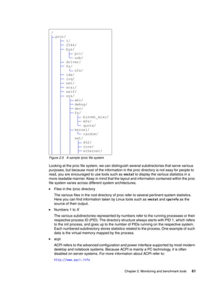
2.3.16 Proc file system
The proc file system is not a real file system, but nevertheless it is extremely useful. It is not
intended to store data; rather, it provides an interface to the running kernel. The proc file
system enables an administrator to monitor and change the kernel on the fly. Figure 2-5 on
page 61 depicts a sample proc file system. Most Linux tools for performance measurement
rely on the information provided by /proc.

75. Chapter 2. Monitoring and benchmark tools 61
Figure 2-5 A sample /proc file system
Looking at the proc file system, we can distinguish several subdirectories that serve various
purposes, but because most of the information in the proc directory is not easy for people to
read, you are encouraged to use tools such as vmstat to display the various statistics in a
more readable manner. Keep in mind that the layout and information contained within the proc
file system varies across different system architectures.
򐂰 Files in the /proc directory
The various files in the root directory of proc refer to several pertinent system statistics.
Here you can find information taken by Linux tools such as vmstat and cpuinfo as the
source of their output.
򐂰 Numbers 1 to X
The various subdirectories represented by numbers refer to the running processes or their
respective process ID (PID). The directory structure always starts with PID 1, which refers
to the init process, and goes up to the number of PIDs running on the respective system.
Each numbered subdirectory stores statistics related to the process. One example of such
data is the virtual memory mapped by the process.
򐂰 acpi
ACPI refers to the advanced configuration and power interface supported by most modern
desktop and notebook systems. Because ACPI is mainly a PC technology, it is often
disabled on server systems. For more information about ACPI refer to:
http://www.apci.info
/
proc/
1/
2546/
bus/
pci/
usb/
driver/
fs/
nfs/
ide/
irq/
net/
scsi/
self/
sys/
abi/
debug/
dev/
fs/
binvmt_misc/
mfs/
quota/
kernel/
random/
net/
802/
core/
ethernet/

76. 62 Linux Performance and Tuning Guidelines
򐂰 bus
This subdirectory contains information about the bus subsystems such as the PCI bus or
the USB interface of the respective system.
򐂰 irq
The irq subdirectory contains information about the interrupts in a system. Each
subdirectory in this directory refers to an interrupt and possibly to an attached device such
as a network interface card. In the irq subdirectory, you can change the CPU affinity of a
given interrupt (a feature we cover later in this book).
򐂰 net
The net subdirectory contains a significant number of raw statistics regarding your network
interfaces, such as received multicast packets or the routes per interface.
򐂰 scsi
This subdirectory contains information about the SCSI subsystem of the respective
system, such as attached devices or driver revision. The subdirectory ips refers to the IBM
ServeRAID controllers found on most IBM System x servers.
򐂰 sys
In the sys subdirectory you find the tunable kernel parameters such as the behavior of the
virtual memory manager or the network stack. We cover the various options and tunable
values in /proc/sys in 4.3, “Changing kernel parameters” on page 104.
򐂰 tty
The tty subdirectory contains information about the respective virtual terminals of the
systems and to what physical devices they are attached.
2.3.17 KDE System Guard
KDE System Guard (KSysguard) is the KDE task manager and performance monitor. It
features a client/server architecture that enables monitoring of local and remote hosts.

77. Chapter 2. Monitoring and benchmark tools 63
Figure 2-6 Default KDE System Guard window
The graphical front end (Figure 2-6) uses sensors to retrieve the information it displays. A
sensor can return simple values or more complex information such as tables. For each type of
information, one or more displays are provided. Displays are organized in work sheets that
can be saved and loaded independent of each other.
The KSysguard main window consists of a menu bar, an optional tool bar and status bar, the
sensor browser, and the workspace. When first started, you see the default setup: your local
machine listed as localhost in the sensor browser and two tabs in the workspace area.
Each sensor monitors a certain system value. All of the displayed sensors can be dragged
and dropped into the work space. There are three options:
򐂰 You can delete and replace sensors in the actual workspace.
򐂰 You can edit work sheet properties and increase the number of rows and columns.
򐂰 You can create a new work sheet and drop new sensors meeting your needs.
Workspace
The workspace in Figure 2-7 on page 64 shows two tabs:
򐂰 System Load, the default view when first starting up KSysguard
򐂰 Process Table

78. 64 Linux Performance and Tuning Guidelines
Figure 2-7 KDE System Guard sensor browser
System Load
The System Load work sheet shows four sensor windows: CPU Load, Load Average (1 Min),
Physical Memory, and Swap Memory. Multiple sensors can be displayed in one window. To
see which sensors are being monitored in a window, mouse over the graph and descriptive
text will appear. You can also right-click the graph and click Properties, then click the
Sensors tab (Figure 2-8). This also shows a key of what each color represents on the graph.
Figure 2-8 Sensor Information, Physical Memory Signal Plotter

79. Chapter 2. Monitoring and benchmark tools 65
Process Table
Clicking the Process Table tab displays information about all running processes on the
server (Figure 2-9). The table, by default, is sorted by System CPU utilization, but this can be
changed by clicking another one of the headings.
Figure 2-9 Process Table view
Configuring a work sheet
For your environment or the particular area that you wish to monitor, you might have to use
different sensors for monitoring. The best way to do this is to create a custom work sheet. In
this section, we guide you through the steps that are required to create the work sheet shown
in Figure 2-12 on page 67:
1. Create a blank work sheet by clicking File → New to open the window in Figure 2-10.
Figure 2-10 Properties for new work sheet
2. Enter a title and a number of rows and columns; this gives you the maximum number of
monitor windows, which in our case will be four. When the information is complete, click
OK to create the blank work sheet, as shown in Figure 2-11 on page 66.

80. 66 Linux Performance and Tuning Guidelines
Figure 2-11 Empty work sheet
3. Fill in the sensor boxes by dragging the sensors on the left side of the window to the
desired box on the right. The types of display are:
– Signal Plotter: This displays samples of one or more sensors over time. If several
sensors are displayed, the values are layered in different colors. If the display is large
enough, a grid will be displayed to show the range of the plotted samples.
By default, the automatic range mode is active, so the minimum and maximum values
will be set automatically. If you want fixed minimum and maximum values, you can
deactivate the automatic range mode and set the values in the Scales tab from the
Properties dialog window (which you access by right-clicking the graph).
– Multimeter: This displays the sensor values as a digital meter. In the Properties dialog,
you can specify a lower and upper limit. If the range is exceeded, the display is colored
in the alarm color.
– BarGraph: This displays the sensor value as dancing bars. In the Properties dialog,
you can specify the minimum and maximum values of the range and a lower and upper
limit. If the range is exceeded, the display is colored in the alarm color.
– Sensor Logger: This does not display any values, but logs them in a file with additional
date and time information.
For each sensor, you have to define a target log file, the time interval the sensor will be
logged, and whether alarms are enabled.
4. Click File → Save to save the changes to the work sheet.
Note: The fastest update interval that can be defined is two seconds.
Note: When you save a work sheet, it will be saved in the user’s home directory, which may
prevent other administrators from using your custom work sheets.

81. Chapter 2. Monitoring and benchmark tools 67
Figure 2-12 Example work sheet
Find more information about KDE System Guard at:
http://docs.kde.org/
2.3.18 Gnome System Monitor
Although not as powerful as the KDE System Guard, the Gnome desktop environment
features a graphical performance analysis tool. The Gnome System Monitor can display
performance-relevant system resources as graphs for visualizing possible peaks and
bottlenecks. Note that all statistics are generated in real time. Long-term performance
analysis should be carried out with different tools.
2.3.19 Capacity Manager
Capacity Manager, an add-on to the IBM Director system management suite for IBM
Systems, is available in the ServerPlus Pack for IBM System x systems. Capacity Manager
offers the possibility of long-term performance measurements across multiple systems and
platforms. Capacity Manager enables capacity planning, offering you an estimate of future
required system capacity needs. With Capacity Manager, you can export reports to HTML,
XML, and GIF files that can be stored automatically on an intranet Web server. IBM Director
can be used on different operating system platforms, which makes it much easier to collect
and analyze data in a heterogeneous environment. Capacity Manager is discussed in detail in
Tuning IBM System x Servers for Performance, SG24-5287.
To use Capacity Manager, you must install the respective RPM package on the systems that
will use its advanced features. After installing the RPM, select Capacity Manager → Monitor
Activator in the IBM Director Console.

82. 68 Linux Performance and Tuning Guidelines
Figure 2-13 The task list in the IBM Director Console
Drag and drop the icon for Monitor Activator over a single system or a group of systems that
have the Capacity Manager package installed. A window opens (Figure 2-14) in which you
can select the various subsystems to be monitored over time. Capacity Manager for Linux
does not yet support the full-feature set of available performance counters. System statistics
are limited to a basic subset of performance parameters.
Figure 2-14 Activating performance monitors multiple systems
The Monitor Activator window shows the respective systems with their current status on the
right side and the different available performance monitors on the left. To add a new monitor,
select the monitor and click On. The changes take effect shortly after the Monitor Activator
window is closed. After this step, IBM Director starts collecting the requested performance
metrics and stores them in a temporary location on the different systems.
To create a report of the collected data, select Capacity Manager → Report Generator (see
Figure 2-13) and drag it over a single system or a group of systems for which you would like to
see performance statistics. IBM Director asks whether the report should be generated
immediately or scheduled for later execution (Figure 2-15 on page 69).

83. Chapter 2. Monitoring and benchmark tools 69
Figure 2-15 Scheduling reports
In a production environment, it is a good idea to have Capacity Manager generate reports on
a regular basis. Our experience is that weekly reports that are performed in off hours over the
weekend can be very valuable. An immediate execution or scheduled execution report is
generated according to your choice. As soon as the report has completed, it is stored on the
central IBM Director management server, where it can be viewed using the Report Viewer
task. Figure 2-16 on page 70 shows sample output from a monthly Capacity Manager report.

84. 70 Linux Performance and Tuning Guidelines
Figure 2-16 A sample Capacity Manager report
The Report Viewer window lets you select different performance counters that were collected
and correlate this data to a single system or to a selection of systems.
Data acquired by Capacity Manager can be exported to an HTML or XML file to be displayed
on an intranet Web server or for future analysis.
2.4 Benchmark tools
In this section we discuss major benchmark tools. To measure performance it’s wise to use
good benchmark tools. There are a lot of good tools available. Some of them have all or some
of the following capabilities:
򐂰 Load generation
򐂰 Monitor performance
򐂰 Monitor system utilization
򐂰 Reporting
A benchmark is nothing more than a model for a specific workload that might or might not be
close to the workload that will run on a system. If a system boasts a good Linpack score it still
might not be the ideal file server. You should always remember that a benchmark cannot
simulate the sometimes unpredictable reactions of an end-user. A benchmark will not tell you
how a file server behaves once the user accesses their data or the backup starts up.
Generally, the following rules should be observed when performing a benchmark on any
system:
򐂰 Use a benchmark for server workloads: Server systems boast distinct characteristics that
make them very different from a typical desktop PC even though the IBM System x

85. Chapter 2. Monitoring and benchmark tools 71
platform shares many of the technologies available for desktop computers. Server
benchmarks spawn multiple threads in order to utilize the SMP capabilities of the system
and in order to simulate a true multi-user environment. While a PC might start one Web
browser faster than a high-end server, the server will start a thousand Web browsers
faster than a PC.
򐂰 Simulate the expected workload: All benchmarks have different configuration options that
should be used to tailor the benchmark towards the workload that the system should be
running in the future. Great CPU performance will be of little use if the application has to
rely on low disk latency.
򐂰 Isolate benchmark systems: If a system is to be tested with a benchmark it is paramount
to isolate it from any other load as much as possible. An open session running the top
command can greatly impact the results of the benchmark.
򐂰 Average results: Even if you try to isolate the benchmark system there might be unknown
factors that could impact systems performance just at the time of your benchmark. It is
good practice to run any benchmark at least three times and average the results in order
to make sure that a one time event does not impact your entire analysis.
In the following sections, we’ve selected some tools based on these criteria:
򐂰 Works on Linux: Linux is the target of the benchmark.
򐂰 Works on all hardware platforms: Since IBM offers three distinct hardware platforms
(assuming that the hardware technology of IBM System p and IBM System i™ are both
based on the IBM POWER™ architecture) it is important to select a benchmark that can
be used without big porting efforts on all architectures.
򐂰 Open source: Linux runs on several platforms, so the binary file might not be available if
the source code is not available.
򐂰 Well-documented: You must know the tool when you perform benchmarking. The
documentation will help you become familiar with the tools. It also helps to evaluate
whether the tool is suited to your needs by taking a look at the concept, design, and details
before you decide to use certain tools.
򐂰 Actively-maintained: The old abandoned tool might not follow the recent specifications and
technologies. It might produce a wrong result.
򐂰 Widely used: You can find a lot of information about widely used tools.
򐂰 Easy to use: You want a tool that’s easy to use.
򐂰 Reporting capability: Having reporting capability will greatly reduce the performance
analysis work.
2.4.1 LMbench
LMbench is a suite of microbenchmarks that can be used to analyze different operating
system settings such as an SELinux enabled system versus a non SELinux system. The
benchmarks included in LMbench measure various operating system routines such as
context switching, local communications, memory bandwidth, and file operations. Using
LMbench is pretty straight forward as there are only three important commands to know;
򐂰 make results: The first time LMbench is run it will prompt for some details of the system
configuration and what tests it should perform.
򐂰 make rerun: After the initial configuration and a first benchmark run, using the make rerun
command simply repeats the benchmark using the configuration supplied during the make
results run.

86. 72 Linux Performance and Tuning Guidelines
򐂰 make see: Finally after a minimum of three runs the results can be viewed using the make
see command. The results will be displayed and can be copied to a spreadsheet
application for further analysis or graphical representation of the data.
The LMbench benchmark can be found at http://sourceforge.net/projects/lmbench/
2.4.2 IOzone
IOzone is a file system benchmark that can be utilized to simulate a wide variety of different
disk access patterns. Since the configuration possibilities of IOzone are detailed, it is possible
to simulate a targeted workload profile precisely. IOzone writes one or multiple files of variable
size using variable block sizes.
While IOzone offers a very comfortable automatic benchmarking mode it is usually more
efficient to define the workload characteristics such as file size, I/O size, and access pattern.
If a file system has to be evaluated for a database workload it would be logical to have IOzone
create a random access pattern to a large file at large block sizes instead of streaming a large
file with a small block size. Some of the most important options for IOzone are:
-b <output.xls> Tells IOzone to store the results in a Microsoft® Excel® compatible
spreadsheet.
-C Displays output for each child process (can be used to check if all
children really run simultaneously).
-f <filename> Can be used to tell IOzone where to write the data.
-i <number of test> This option is used to specify what tests are to be run. You will always
have to specify -i 0 in order to write the test file for the first time.
Useful tests are -i 1 for streaming reads, -i 2 for random read and
random write access, and -i 8 for a workload with mixed random
access.
-h Displays the onscreen help.
-r Tells IOzone what record or I/O size that should be used for the tests.
The record size should be as close as possible to the record size that
will be used by the targeted workload.
-k <number of async I/Os>
Uses the async I/O feature of kernel 2.6 that is often used by
databases such as IBM DB2®.
-m If the targeted application uses multiple internal buffers then this
behavior can be simulated using the -m flag.
-s <size in KB> Specifies the file size for the benchmark. For asynchronous file
systems (the default mounting option for most file systems) IOzone
should be used with a file size of at least twice the system’s memory in
order to really measure disk performance. The size can also be
specified in MB or GB using m or g respectively, directly after the file
size.
-+u Is an experimental switch that can be used to measure the processor
utilization during the test.
Note: Any benchmark using files that fit into the system’s memory and that are stored on
asynchronous file systems will measure the memory throughput rather than the disk
subsystem performance. So, you should either mount the file system of interest with the
sync option or use a file size roughly twice the size of the system’s memory.

87. Chapter 2. Monitoring and benchmark tools 73
Using IOzone to measure the random read performance of a given disk subsystem mounted
at /perf for a file of 10 GB size at 32 KB I/O size (these characteristics model a simple
database) would look as follows:
Example 2-26 A sample IOzone command line
./iozone -b results.xls -R -i 0 -i 2 -f /perf/iozone.file -r 32 -s 10g
Finally, the obtained result can be imported into your spreadsheet application of choice and
then transformed into graphs. Using a graphical output of the data might make it easier to
analyze a large amount of data and to identify trends. A sample output of Example 2-26 might
look like the graphic displayed in Figure 2-17.
Figure 2-17 A graphic produced out of the sample results of Example 2-26
If IOzone is used with file sizes that either fit into the system’s memory or cache it can also be
used to gain some data about cache and memory throughput. It should be noted that due to
the file system overheads IOzone will report only 70-80% of a system’s bandwidth.
The IOzone benchmark can be found at http://www.iozone.org/
2.4.3 netperf
netperf is a performance benchmark tool that focuses on TCP/IP networking performance. It
supports UNIX domain socket and SCTP benchmarking.
netperf is designed based on a client-server model. netserver runs on a target system and
netperf runs on the client. netperf controls the netserver and passes configuration data to
netserver, generates network traffic, and gets the result from netserver through a control
connection that is separated from the actual benchmark traffic connection. During the
benchmarking, no communication occurs on the control connection so it does not have any
effect on the result. The netperf benchmark tool also has a reporting capability including a
CPU utilization report. The current stable version is 2.4.3 at the time of writing.
0
20000
40000
60000
80000
100000
120000
kB/sec
Writer Report Re-writer Report Random Read
Report
Random Write
Report
10 GB File Access at 32 KB I/O Size

88. 74 Linux Performance and Tuning Guidelines
netperf can generate several types of traffic. Basically these fall into two categories: bulk
data transfer traffic and request/response type traffic. You should note that netperf uses only
one socket at a time. The next version of netperf (netperf4) will fully support benchmarking for
concurrent sessions. At this time, we can perform multiple session benchmarking as
described below.
򐂰 Bulk data transfer
Bulk data transfer is the most commonly measured factor in network benchmarking. The
bulk data transfer is measured by the amount of data transferred in one second. It
simulates large file transfer such as multimedia streaming and FTP data transfer.
򐂰 Request/response type
This simulates request/response type traffic which is measured by the number of
transactions exchanged in one second. Request/response traffic type is typical for online
transaction applications such as web server, database server, mail server, file server
(which serves small or medium files), and directory server. In real environment, session
establishment and termination should be performed as well as data exchange. To simulate
this, TCP_CRR type was introduced.
򐂰 Concurrent session
netperf does not have real support for concurrent multiple session benchmarking in the
current stable version, but we can perform some benchmarking by just issuing multiple
instances of netperf as follows:
for i in ‘seq 1 10‘; do netperf -t TCP_CRR -H target.example.com -i 10 -P 0
&; done
We’ll look at some useful and interesting options.
Global options:
-A Change send and receive buffer alignment on remote system
-b Burst of packet in stream test
-H <remotehost> Remote host
-t <testname> Test traffic type
TCP_STREAM Bulk data transfer benchmark
TCP_MAERTS Similar to TCP_STREAM except direction of stream is opposite.
TCP_SENDFILE Similar to TCP_STREAM except using sendfile() instead of
send(). It causes a zero-copy operation.
UDP_STREAM Same as TCP_STREAM except UDP is used.
TCP_RR Request/response type traffic benchmark
TCP_CC TCP connect/close benchmark. No request and response packet is
exchanged.
TCP_CRR Performs connect/request/response/close operation. It is very
similar to HTTP1.0/1.1 session with HTTP keepalive disabled.
UDP_RR Same as TCP_RR except UDP is used.
-l <testlen> Test length of benchmarking. If positive value is set, netperf performs
the benchmarking in testlen seconds. If negative, it performs until
value of testlen bytes of data is exchanged for bulk data transfer
benchmarking or value of testlen transactions for request/response
type.
-c Local CPU utilization report

89. Chapter 2. Monitoring and benchmark tools 75
-C Remote CPU utilization report
-I <conflevel><interval>
This option is used to maintain confidence of the result. The
confidence level should be 99 or 95 (percent) and interval (percent)
can be set. To keep the result at a certain level of confidence, the
netperf repeats the same benchmarking several times. For example,
-I 99,5 means that the result is within 5% interval (+- 2.5%) of the real
result in 99 times out of 100.
-i <max><min> Number of maximum and minimum test iterations. This option limits
the number of iterations. -i 10,3 means netperf performs the same
benchmarking at least 3 times and at most 10 times. If the iteration
exceeds the maximum value, the result would not be in the confidence
level which is specified with -I option, and a warning will be displayed
in the result.
-s <bytes>, -S <bytes>
Changes send and receive buffer size on local, remote system. This
will affect the advertised and effective window size.
Options for TCP_STREAM, TCP_MAERTS, TCP_SENDFILE, UDP_STREAM
-m <bytes>, -M <bytes>
Specifies the size of buffer passed to send(), recv() function call
respectively and controls the size sent and received per call.
Options for TCP_RR, TCP_CC, TCP_CRR, UDP_RR:
-r <bytes>, -R <bytes>
Specifies request, response size respectively. For example, -r
128,8129 means that netperf sends 128 byte packets to the netserver
and it sends the 8129 byte packets back to netperf.
The following is an example output of netperf for TCP_CRR type benchmark.
Example 2-27 An example result of TCP_CRR benchmark
Testing with the following command line:
/usr/local/bin/netperf -l 60 -H plnxsu4 -t TCP_CRR -c 100 -C 100 -i ,3 -I 95,5 -v
1 -- -r 64,1 -s 0 -S 512
TCP Connect/Request/Response TEST from 0.0.0.0 (0.0.0.0) port 0 AF_INET to plnxsu4
(10.0.0.4) port 0 AF_INET
Local /Remote
Socket Size Request Resp. Elapsed Trans. CPU CPU S.dem S.dem
Send Recv Size Size Time Rate local remote local remote
bytes bytes bytes bytes secs. per sec % % us/Tr us/Tr
16384 87380 64 1 60.00 3830.65 25.27 10.16 131.928 53.039
2048 1024
When you perform benchmarking, it’s wise to use the sample test scripts which come with
netperf. By changing some variables in the scripts, you can perform your benchmarking as
you like. The scripts are in the doc/examples/ directory of the netperf package.
Note: The report of the CPU utilization might not be accurate in some platforms. Make
sure it is accurate before you perform benchmarking.

90. 76 Linux Performance and Tuning Guidelines
For more details, refer to http://www.netperf.org/
2.4.4 Other useful tools
Here are some other useful benchmark tools. Keep in mind that you have to know the
characteristics of the benchmark tools so that you can choose the tools that fit your needs.
Table 2-3 Additional benchmarking tools
Tool Most useful tool function
bonnie Disk I/O and file system benchmark
http://www.textuality.com/bonnie/
bonnie++ Disk I/O and file system benchmark
http://www.coker.com.au/bonnie++/
NetBench File server benchmark. It runs on Windows.
dbench File system benchmark. Commonly used for file server benchmark.
http://freshmeat.net/projects/dbench/
iometer Disk I/O and network benchmark
http://www.iometer.org/
ttcp Simple network benchmark
nttcp Simple network benchmark
iperf Network benchmark
http://dast.nlanr.net/projects/Iperf/
ab (Apache Bench) Simple web server benchmark. It comes with Apache HTTP server.
http://httpd.apache.org/
WebStone Web server benchmark
http://www.mindcraft.com/webstone/
Apache JMeter Used mainly for web server performance benchmarking. It also
support other protocol such as SMTP, LDAP, JDBC™ and so on, and
it has good reporting capability.
http://jakarta.apache.org/jmeter/
fsstone, smtpstone Mail server benchmark. They come with Postfix.
http://www.postfix.org/
nhfsstone Network File System benchmark. Comes with nfs-utils package.
DirectoryMark LDAP benchmark
http://www.mindcraft.com/directorymark/

91. © Copyright IBM Corp. 2007. All rights reserved. 77
Chapter 3. Analyzing performance
bottlenecks
This chapter explains how to find a performance problem that might be affecting one of your
servers. We outline a series of steps to lead you to a concrete solution that you can
implement to restore the server to an acceptable performance level.
The topics that are covered in this chapter are:
򐂰 3.1, “Identifying bottlenecks” on page 78
򐂰 3.2, “CPU bottlenecks” on page 81
򐂰 3.3, “Memory bottlenecks” on page 82
򐂰 3.4, “Disk bottlenecks” on page 84
򐂰 3.5, “Network bottlenecks” on page 87
3

92. 78 Linux Performance and Tuning Guidelines
3.1 Identifying bottlenecks
The following steps are used as our quick tuning strategy:
1. Know your system.
2. Back up the system.
3. Monitor and analyze the system’s performance.
4. Narrow down the bottleneck and find its cause.
5. Fix the bottleneck cause by trying one change at a time.
6. Go back to step 3 until you are satisfied with the performance of the system.
3.1.1 Gathering information
Most likely, the only first-hand information you will have access to will be statements such as
“There is a problem with the server.” It is crucial to use probing questions to clarify and
document the problem. Here is a list of questions you should ask to help you get a better
picture of the system.
򐂰 Can you give me a complete description of the server in question?
– Model
– Age
– Configuration
– Peripheral equipment
– Operating system version and update level
򐂰 Can you tell me exactly what the problem is?
– What are the symptoms?
– Describe any error messages.
Some people will have problems answering this question, but any extra information the
customer can give you might help you find the problem. For example, the customer might
say “It is really slow when I copy large files to the server.” This could indicate a network
problem or a disk subsystem problem.
򐂰 Who is experiencing the problem?
Is one person, one particular group of people, or the entire organization experiencing the
problem? This helps determine whether the problem exists in one particular part of the
network, whether it is application-dependent, and so on. If only one user experiences the
problem, then the problem might be with the user’s PC (or their imagination).
The perception clients have of the server is usually a key factor. From this point of view,
performance problems might not be directly related to the server: the network path
between the server and the clients can easily be the cause of the problem. This path
includes network devices as well as services provided by other servers, such as domain
controllers.
򐂰 Can the problem be reproduced?
All reproducible problems can be solved. If you have sufficient knowledge of the system,
you should be able to narrow the problem to its root and decide which actions should be
taken.
Tip: You should document each step, especially the changes you make and their affect on
performance.

93. Chapter 3. Analyzing performance bottlenecks 79
The fact that the problem can be reproduced lets you see and understand it better.
Document the sequence of actions that are necessary to reproduce the problem:
– What are the steps to reproduce the problem?
Knowing the steps might help you reproduce the same problem on a different machine
under the same conditions. If this works, it gives you the opportunity to use a machine
in a test environment and removes the chance of crashing the production server.
– Is it an intermittent problem?
If the problem is intermittent, the first thing to do is to gather information and find a path
to move the problem to the reproducible category. The goal here is to have a scenario
to make the problem happen on command.
– Does it occur at certain times of the day or certain days of the week?
This might help you determine what is causing the problem. It might occur when
everyone arrives for work or returns from lunch. Look for ways to change the timing
(that is, make it happen less or more often); so that the problem becomes reproducible.
– Is it unusual?
If the problem falls into the non-reproducible category, you might conclude that it is the
result of extraordinary conditions and classify it as fixed. In real life, there is a high
probability that it will happen again.
A good procedure to troubleshoot a hard-to-reproduce problem is to perform general
maintenance on the server: reboot, or bring the machine up to date on drivers and
patches.
򐂰 When did the problem start? Was it gradual or did it occur very quickly?
If the performance issue appeared gradually, then it is likely to be a sizing issue; if it
appeared overnight, then the problem could be caused by a change made to the server or
peripherals.
򐂰 Have any changes been made to the server (minor or major) or are there any changes in
the way clients are using the server?
Did the customer alter something on the server or peripherals to cause the problem? Is
there a log of all network changes available?
Demands could change based on business changes, which could affect demands on a server
and network systems.
򐂰 Are there any other servers or hardware components involved?
򐂰 Are any logs available?
򐂰 What is the priority of the problem? When does it have to be fixed?
– Does it have to be fixed in the next few minutes, or in days? You may have some time to
fix it; or it may already be time to operate in panic mode.
– How massive is the problem?
– What is the related cost of that problem?

94. 80 Linux Performance and Tuning Guidelines
3.1.2 Analyzing the server’s performance
At this point, you should begin monitoring the server. The simplest way is to run monitoring
tools from the server that is being analyzed. (See Chapter 2, “Monitoring and benchmark
tools” on page 39, for more information.)
A performance log of the server should be created during its peak time of operation (for
example, 9:00 a.m. to 5:00 p.m.); it will depend on what services are being provided and on
who is using these services. When creating the log, if available, the following objects should
be included:
򐂰 Processor
򐂰 System
򐂰 Server work queues
򐂰 Memory
򐂰 Page file
򐂰 Physical disk
򐂰 Redirector
򐂰 Network interface
Before you begin, remember that a methodical approach to performance tuning is important.
Our recommended process, which you can use for your server performance tuning process,
is as follows:
1. Understand the factors affecting server performance.
2. Measure the current performance to create a performance baseline to compare with your
future measurements and to identify system bottlenecks.
3. Use the monitoring tools to identify a performance bottleneck. By following the instructions
in the next sections, you should be able to narrow down the bottleneck to the subsystem
level.
4. Work with the component that is causing the bottleneck by performing some actions to
improve server performance in response to demands.
5. Measure the new performance. This helps you compare performance before and after the
tuning steps.
When attempting to fix a performance problem, remember the following:
򐂰 Applications should be compiled with an appropriate optimization level to reduce the path
length.
򐂰 Take measurements before you upgrade or modify anything so that you can tell whether
the change had any effect. (That is, take baseline measurements.)
򐂰 Examine the options that involve reconfiguring existing hardware, not just those that
involve adding new hardware.
Important: Before taking any troubleshooting actions, back up all data and the
configuration information to prevent a partial or complete loss.
Note: It is important to understand that the greatest gains are obtained by upgrading a
component that has a bottleneck when the other components in the server have ample
“power” left to sustain an elevated level of performance.

95. Chapter 3. Analyzing performance bottlenecks 81
3.2 CPU bottlenecks
For servers whose primary role is that of an application or database server, the CPU is a
critical resource and can often be a source of performance bottlenecks. It is important to note
that high CPU utilization does not always mean that a CPU is busy doing work; it might be
waiting on another subsystem. When performing proper analysis, it is very important that you
look at the system as a whole and at all subsystems because there could be a cascade effect
within the subsystems.
3.2.1 Finding CPU bottlenecks
Determining bottlenecks with the CPU can be accomplished in several ways. As discussed in
Chapter 2, “Monitoring and benchmark tools” on page 39, Linux has a variety of tools to help
determine this. The question is which tools to use.
One tool is uptime. By analyzing the output from uptime, we can get a rough idea of what has
been happening in the system for the past 15 minutes. For a more detailed explanation of this
tool, see 2.3.3, “uptime” on page 43.
Example 3-1 uptime output from a CPU strapped system
18:03:16 up 1 day, 2:46, 6 users, load average: 182.53, 92.02, 37.95
Using KDE System Guard and the CPU sensors lets you view the current CPU workload.
Using top, you can see the CPU utilization and what processes are the biggest contributors to
the problem (Example 2-1 on page 41). If you have set up sar, you are collecting a lot of
information, some of which is CPU utilization, over a period of time. Analyzing this information
can be difficult, so use isag, which can use sar output to plot a graph. Otherwise, you may
wish to parse the information through a script and use a spreadsheet to plot it to see any
trends in CPU utilization. You can also use sar from the command line by issuing sar -u or
sar -U processornumber. To gain a broader perspective of the system and current utilization
of more than just the CPU subsystem, a good tool is vmstat (see 2.3.2, “vmstat” on page 42
for more information).
3.2.2 SMP
SMP-based systems can present their own set of interesting problems that can be difficult to
detect. In an SMP environment, there is the concept of CPU affinity, which implies that you
bind a process to a CPU.
The main reason this is useful is because of CPU cache optimization, which is achieved by
keeping the same process on one CPU rather than moving between processors. When a
process moves between CPUs, the cache of the new CPU must be flushed. Therefore, a
process that moves between processors causes many cache flushes to occur, which means
Note: There is a common misconception that the CPU is the most important part of the
server. This is not always the case, and servers are often overconfigured with CPU and
underconfigured with disks, memory, and network subsystems. Only specific applications
that are truly CPU intensive can take advantage of today’s high-end processors.
Tip: Be careful not to add to CPU problems by running too many tools at one time. You
might find that using a lot of different monitoring tools at one time could be contributing to
the high CPU load.

96. 82 Linux Performance and Tuning Guidelines
that an individual process will take longer to finish. This scenario is very hard to detect
because, when monitoring it, the CPU load will appear to be very balanced and not
necessarily peaking on any CPU. Affinity is also useful in NUMA-based systems such as the
IBM System x 3950, where it is important to keep memory, cache, and CPU access local to
one another.
3.2.3 Performance tuning options
The first step is to ensure that the system performance problem is being caused by the CPU
and not one of the other subsystems. If the processor is the server bottleneck, then a number
of actions can be taken to improve performance. These include:
򐂰 Ensure that no unnecessary programs are running in the background by using ps -ef. If
you find such programs, stop them and use cron to schedule them to run at off-peak
hours.
򐂰 Identify non-critical, CPU-intensive processes by using top and modify their priority using
renice.
򐂰 In an SMP-based machine, try using taskset to bind processes to CPUs to make sure that
processes are not hopping between processors, causing cache flushes.
򐂰 Based on the running application, it might be better to scale up (bigger CPUs) than to
scale out (more CPUs). This depends on whether or not your application was designed to
effectively take advantage of more processors. For example, a single-threaded application
would scale better with a faster CPU and not with more CPUs.
򐂰 General options include making sure you are using the latest drivers and firmware,
because this could affect the load they have on the CPU.
3.3 Memory bottlenecks
On a Linux system, many programs run at the same time. These programs support multiple
users, and some processes are more used than others. Some of these programs use a
portion of memory while the rest are “sleeping.” When an application accesses cache, the
performance increases because an in-memory access retrieves data, thereby eliminating the
need to access slower disks.
The OS uses an algorithm to control which programs will use physical memory and which are
paged out. This is transparent to user programs. Page space is a file created by the OS on a
disk partition to store user programs that are not currently in use. Typically, page sizes are
4 KB or 8 KB. In Linux, the page size is defined by using the variable EXEC_PAGESIZE in the
include/asm-<architecture>/param.h kernel header file. The process used to page a process
out to disk is called pageout.
3.3.1 Finding memory bottlenecks
Start your analysis by listing the applications that are running on the server. Determine how
much physical memory and swap each application needs to run. Figure 3-1 on page 83
shows KDE System Guard monitoring memory usage.

97. Chapter 3. Analyzing performance bottlenecks 83
Figure 3-1 KDE System Guard memory monitoring
The indicators in Table 3-1 can also help you define a problem with memory.
Table 3-1 Indicator for memory analysis
Paging and swapping indicators
In Linux, as with all UNIX-based operating systems, there are differences between paging
and swapping. Paging moves individual pages to swap space on the disk; swapping is a
bigger operation that moves the entire address space of a process to swap space in one
operation.
Swapping can have one of two causes:
򐂰 A process enters sleep mode. This usually happens because the process depends on
interactive action and editors, shells, and data entry applications spend most of their time
waiting for user input. During this time, they are inactive.
Memory indicator Analysis
Memory available This indicates how much physical memory is available for use. If, after you start your application,
this value has decreased significantly, you might have a memory leak. Check the application that
is causing it and make the necessary adjustments. Use free -l -t -o for additional information.
Page faults There are two types of page faults: soft page faults, when the page is found in memory, and hard
page faults, when the page is not found in memory and must be fetched from disk. Accessing
the disk will slow your application considerably. The sar -B command can provide useful
information for analyzing page faults, specifically columns pgpgin/s and pgpgout/s.
File system cache This is the common memory space used by the file system cache. Use the free -l -t -o
command for additional information.
Private memory for
process
This represents the memory used by each process running on the server. You can use the pmap
command to see how much memory is allocated to a specific process.

98. 84 Linux Performance and Tuning Guidelines
򐂰 A process behaves poorly. Paging can be a serious performance problem when the
amount of free memory pages falls below the minimum amount specified, because the
paging mechanism is not able to handle the requests for physical memory pages and the
swap mechanism is called to free more pages. This significantly increases I/O to disk and
will quickly degrade a server’s performance.
If your server is always paging to disk (a high page-out rate), consider adding more memory.
However, for systems with a low page-out rate, it might not affect performance.
3.3.2 Performance tuning options
It you believe there is a memory bottleneck, consider performing one or more of these
actions:
򐂰 Tune the swap space using bigpages, hugetlb, shared memory.
򐂰 Increase or decrease the size of pages.
򐂰 Improve the handling of active and inactive memory.
򐂰 Adjust the page-out rate.
򐂰 Limit the resources used for each user on the server.
򐂰 Stop the services that are not needed, as discussed in “Daemons” on page 97.
򐂰 Add memory.
3.4 Disk bottlenecks
The disk subsystem is often the most important aspect of server performance and is usually
the most common bottleneck. However, problems can be hidden by other factors, such as
lack of memory. Applications are considered to be I/O-bound when CPU cycles are wasted
simply waiting for I/O tasks to finish.
The most common disk bottleneck is having too few disks. Most disk configurations are based
on capacity requirements, not performance. The least expensive solution is to purchase the
smallest number of the largest capacity disks possible. However, this places more user data
on each disk, causing greater I/O rates to the physical disk and allowing disk bottlenecks to
occur.
The second most common problem is having too many logical disks on the same array. This
increases seek time and significantly lowers performance.
The disk subsystem is discussed in 4.6, “Tuning the disk subsystem” on page 112.
3.4.1 Finding disk bottlenecks
A server exhibiting the following symptoms might be suffering from a disk bottleneck (or a
hidden memory problem):
򐂰 Slow disks will result in:
– Memory buffers filling with write data (or waiting for read data), which will delay all
requests because free memory buffers are unavailable for write requests (or the
response is waiting for read data in the disk queue).
– Insufficient memory, as in the case of not enough memory buffers for network requests,
will cause synchronous disk I/O.
򐂰 Disk utilization, controller utilization, or both will typically be very high.
򐂰 Most LAN transfers will happen only after disk I/O has completed, causing very long
response times and low network utilization.

99. Chapter 3. Analyzing performance bottlenecks 85
򐂰 Disk I/O can take a relatively long time and disk queues will become full, so the CPUs will
be idle or have low utilization because they wait long periods of time before processing the
next request.
The disk subsystem is perhaps the most challenging subsystem to properly configure.
Besides looking at raw disk interface speed and disk capacity, it is also important to
understand the workload. Is disk access random or sequential? Is there large I/O or small
I/O? Answering these questions provides the necessary information to make sure the disk
subsystem is adequately tuned.
Disk manufacturers tend to showcase the upper limits of their drive technology’s throughput.
However, taking the time to understand the throughput of your workload will help you
understand what true expectations to have of your underlying disk subsystem.
Table 3-2 Exercise showing true throughput for 8 KB I/Os for different drive speeds
Random read/write workloads usually require several disks to scale. The bus bandwidths of
SCSI or Fibre Channel are of lesser concern. Larger databases with random access
workload will benefit from having more disks. Larger SMP servers will scale better with more
disks. Given the I/O profile of 70% reads and 30% writes of the average commercial
workload, a RAID-10 implementation will perform 50% to 60% better than a RAID-5.
Sequential workloads tend to stress the bus bandwidth of disk subsystems. Pay special
attention to the number of SCSI buses and Fibre Channel controllers when maximum
throughput is desired. Given the same number of drives in an array, RAID-10, RAID-0, and
RAID-5 all have similar streaming read and write throughput.
There are two ways to approach disk bottleneck analysis: real-time monitoring and tracing.
򐂰 Real-time monitoring must be done while the problem is occurring. This might not be
practical in cases where system workload is dynamic and the problem is not repeatable.
However, if the problem is repeatable, this method is flexible because of the ability to add
objects and counters as the problem becomes clear.
򐂰 Tracing is the collecting of performance data over time to diagnose a problem. This is a
good way to perform remote performance analysis. Some of the drawbacks include the
potential for having to analyze large files when performance problems are not repeatable,
and the potential for not having all key objects and parameters in the trace and having to
wait for the next time the problem occurs for the additional data.
vmstat command
One way to track disk usage on a Linux system is by using the vmstat tool. The important
columns in vmstat with respect to I/O are the bi and bo fields. These fields monitor the
movement of blocks in and out of the disk subsystem. Having a baseline is key to being able
to identify any changes over time.
Disk speed Latency Seek
time
Total random
access timea
a. Assuming that the handling of the command + data transfer < 1 ms, total random
access time = latency + seek time + 1 ms
I/Os per
second
per diskb
b. Calculated as 1/total random access time
Throughput
given 8 KB I/O
15 000 RPM 2.0 ms 3.8 ms 6.8 ms 147 1.15 MBps
10 000 RPM 3.0 ms 4.9 ms 8.9 ms 112 900 KBps
7 200 RPM 4.2 ms 9 ms 13.2 ms 75 600 KBps

100. 86 Linux Performance and Tuning Guidelines
Example 3-2 vmstat output
[root@x232 root]# vmstat 2
r b swpd free buff cache si so bi bo in cs us sy id wa
2 1 0 9004 47196 1141672 0 0 0 950 149 74 87 13 0 0
0 2 0 9672 47224 1140924 0 0 12 42392 189 65 88 10 0 1
0 2 0 9276 47224 1141308 0 0 448 0 144 28 0 0 0 100
0 2 0 9160 47224 1141424 0 0 448 1764 149 66 0 1 0 99
0 2 0 9272 47224 1141280 0 0 448 60 155 46 0 1 0 99
0 2 0 9180 47228 1141360 0 0 6208 10730 425 413 0 3 0 97
1 0 0 9200 47228 1141340 0 0 11200 6 631 737 0 6 0 94
1 0 0 9756 47228 1140784 0 0 12224 3632 684 763 0 11 0 89
0 2 0 9448 47228 1141092 0 0 5824 25328 403 373 0 3 0 97
0 2 0 9740 47228 1140832 0 0 640 0 159 31 0 0 0 100
iostat command
Performance problems can be encountered when too many files are opened, read and written
to, then closed repeatedly. This could become apparent as seek times (the time it takes to
move to the exact track where the data is stored) start to increase. Using the iostat tool, you
can monitor the I/O device loading in real time. Different options enable you to drill down even
deeper to gather the necessary data.
Example 3-3 shows a potential I/O bottleneck on the device /dev/sdb1. This output shows
average wait times (await) of about 2.7 seconds and service times (svctm) of 270 ms.
Example 3-3 Sample of an I/O bottleneck as shown with iostat 2 -x /dev/sdb1
[root@x232 root]# iostat 2 -x /dev/sdb1
avg-cpu: %user %nice %sys %idle
11.50 0.00 2.00 86.50
Device: rrqm/s wrqm/s r/s w/s rsec/s wsec/s rkB/s wkB/s avgrq-sz
avgqu-sz await svctm %util
/dev/sdb1 441.00 3030.00 7.00 30.50 3584.00 24480.00 1792.00 12240.00 748.37
101.70 2717.33 266.67 100.00
avg-cpu: %user %nice %sys %idle
10.50 0.00 1.00 88.50
Device: rrqm/s wrqm/s r/s w/s rsec/s wsec/s rkB/s wkB/s avgrq-sz
avgqu-sz await svctm %util
/dev/sdb1 441.00 3030.00 7.00 30.00 3584.00 24480.00 1792.00 12240.00 758.49
101.65 2739.19 270.27 100.00
avg-cpu: %user %nice %sys %idle
10.95 0.00 1.00 88.06
Device: rrqm/s wrqm/s r/s w/s rsec/s wsec/s rkB/s wkB/s avgrq-sz
avgqu-sz await svctm %util
/dev/sdb1 438.81 3165.67 6.97 30.35 3566.17 25576.12 1783.08 12788.06 781.01
101.69 2728.00 268.00 100.00
For a more detailed explanation of the fields, see the man page for iostat(1).

101. Chapter 3. Analyzing performance bottlenecks 87
Changes made to the elevator algorithm as described in 4.6.2, “I/O elevator tuning and
selection” on page 115 will be seen in avgrq-sz (average size of request) and avgqu-sz
(average queue length). As the latencies are lowered by manipulating the elevator settings,
avgrq-sz will decrease. You can also monitor the rrqm/s and wrqm/s to see the effect on the
number of merged reads and writes that the disk can manage.
3.4.2 Performance tuning options
After verifying that the disk subsystem is a system bottleneck, several solutions are possible.
These solutions include the following:
򐂰 If the workload is of a sequential nature and it is stressing the controller bandwidth, the
solution is to add a faster disk controller. However, if the workload is more random in
nature, then the bottleneck is likely to involve the disk drives, and adding more drives will
improve performance.
򐂰 Add more disk drives in a RAID environment. This spreads the data across multiple
physical disks and improves performance for both reads and writes. This will increase the
number of I/Os per second. Also, use hardware RAID instead of the software
implementation provided by Linux. If hardware RAID is being used, the RAID level is
hidden from the OS.
򐂰 Consider using Linux logical volumes with striping instead of large single disks or logical
volumes without striping.
򐂰 Offload processing to another system in the network (users, applications, or services).
򐂰 Add more RAM. Adding memory increases system memory disk cache, which in effect
improves disk response times.
3.5 Network bottlenecks
A performance problem in the network subsystem can be the cause of many problems, such
as a kernel panic. To analyze these anomalies to detect network bottlenecks, each Linux
distribution includes traffic analyzers.
3.5.1 Finding network bottlenecks
We recommend KDE System Guard because of its graphical interface and ease of use. The
tool, which is available on the distribution CDs, is discussed in detail in 2.3.17, “KDE System
Guard” on page 62. Figure 3-2 on page 88 shows it in action.

102. 88 Linux Performance and Tuning Guidelines
Figure 3-2 KDE System Guard network monitoring
It is important to remember that there are many possible reasons for these performance
problems and that sometimes problems occur simultaneously, making it even more difficult to
pinpoint the origin. The indicators in Table 3-3 can help you determine the problem with your
network.
Table 3-3 Indicators for network analysis
Network indicator Analysis
Packets received
Packets sent
Shows the number of packets that are coming in and going out of the
specified network interface. Check both internal and external interfaces.
Collision packets Collisions occur when there are many systems on the same domain. The
use of a hub may be the cause of many collisions.
Dropped packets Packets may be dropped for a variety of reasons, but the result can affect
performance. For example, if the server network interface is configured to
run at 100 Mbps full duplex, but the network switch is configured to run at
10 Mbps, the router may have an ACL filter that drops these packets. For
example:
iptables -t filter -A FORWARD -p all -i eth2 -o eth1 -s 172.18.0.0/24
-j DROP
Errors Errors occur if the communication lines (for instance, the phone line) are of
poor quality. In these situations, corrupted packets must be resent, thereby
decreasing network throughput.
Faulty adapters Network slowdowns often result from faulty network adapters. When this
kind of hardware fails, it might begin to broadcast junk packets on the
network.

103. Chapter 3. Analyzing performance bottlenecks 89
3.5.2 Performance tuning options
These steps illustrate what you should do to solve problems related to network bottlenecks:
򐂰 Ensure that the network card configuration matches router and switch configurations (for
example, frame size).
򐂰 Modify how your subnets are organized.
򐂰 Use faster network cards.
򐂰 Tune the appropriate IPV4 TCP kernel parameters. (See Chapter 4, “Tuning the operating
system” on page 91.) Some security-related parameters can also improve performance,
as described in that chapter.
򐂰 If possible, change network cards and recheck performance.
򐂰 Add network cards and bind them together to form an adapter team, if possible.

104. 90 Linux Performance and Tuning Guidelines

105. © Copyright IBM Corp. 2007. All rights reserved. 91
Chapter 4. Tuning the operating system
Linux distributions and the Linux kernel offer a variety of parameters and settings to let the
Linux administrator tweak the system to maximize performance. As stated earlier in this
paper, there is no magic tuning knob that will improve systems performance for any
application. The settings discussed in the following chapter will improve performance for
certain hardware configurations and application layouts. The settings that improve
performance for a Web server scenario might have adverse impacts on the performance of a
database system.
This chapter describes the steps you can take to tune kernel 2.6 based Linux distributions.
Since the current kernel 2.6 based distributions vary from kernel release 2.6.9 up to 2.6.19 (at
the time of this paper) some tuning options might only apply to a specific kernel release. The
objective is to describe the parameters that give you the most improvement in performance
and offer a basic understanding of the techniques that are used in Linux, including:
򐂰 Linux memory management
򐂰 System clean up
򐂰 Disk subsystem tuning
򐂰 Kernel tuning using sysctl
򐂰 Network optimization
This chapter has the following sections:
򐂰 4.1, “Tuning principles” on page 92
򐂰 4.2, “Installation considerations” on page 92
򐂰 4.3, “Changing kernel parameters” on page 104
򐂰 4.4, “Tuning the processor subsystem” on page 107
򐂰 4.5, “Tuning the vm subsystem” on page 109
򐂰 4.6, “Tuning the disk subsystem” on page 112
򐂰 4.7, “Tuning the network subsystem” on page 124
4

106. 92 Linux Performance and Tuning Guidelines
4.1 Tuning principles
Tuning any system should follow some simple principles of which the most important is
change management as described below. Generally the first step in systems tuning should be
to analyze and evaluate the current system configuration. Ensuring that the system performs
as stated by the hardware manufacturer and that all devices are running in their optimal mode
will create a solid base for any later tuning. Also prior to any specific tuning tasks a system
designed for optimal performance should have a minimum of unnecessary tasks and
subsystems running. Finally when moving towards specific systems tuning, it should be noted
that tuning often tailors a system towards a specific workload. So, the system will perform
better under the intended load characteristics but it will probably perform worse for different
workload patterns. An example would be tuning a system for low latency which most of the
time has an adverse effect on throughput.
4.1.1 Change management
While not strictly related to performance tuning, change management is probably the single
most important factor for successful performance tuning. The following considerations might
be second nature to you, but as a reminder we highlight these points:
򐂰 Implement a proper change management process before tuning any Linux system.
򐂰 Never start tweaking settings on a production system.
򐂰 Never change more than one variable during the tuning process.
򐂰 Retest parameters that supposedly improved performance; sometimes statistics come into
play.
򐂰 Document successful parameters and share them with the community no matter how
trivial you think they are. Linux performance can benefit greatly from any results obtained
in production environments.
4.2 Installation considerations
Ideally the tuning of a server system towards a specific performance goal should start with the
design and installation phase. A proper installation that tailors a system towards the workload
pattern will save a significant amount of time during the later tuning phase.
4.2.1 Installation
In a perfect world, tuning of any given system starts at a very early stage. Ideally a system is
tailored to the needs of the application and the anticipated workload. We understand that
most of the time an administrator has to tune an already installed system due to a bottleneck,
but we also want to highlight the tuning possibilities available during the initial installation of
the operating system.
Several issues should be resolved before starting the installation of Linux, including:
򐂰 Selection of the processor technology
򐂰 Choice of disk technology
򐂰 Applications
However, these issues are beyond the scope of this paper.
Ideally, the following questions should be answered before starting the installation:

107. Chapter 4. Tuning the operating system 93
򐂰 What flavor and version of Linux do I need?
After you have collected the business and application requirements, decide which version
of Linux to use. Enterprises often have contractual agreements that allow the general use
of a specific Linux distribution. In this case, financial and contractual benefits will probably
dictate the version of Linux that can be used. However, if you have full freedom in
choosing the version of your Linux distribution, there are some questions to consider:
– A supported Enterprise Linux or a custom made distribution?
In some scientific environments it is acceptable to run an unsupported version of Linux,
such as Fedora. For enterprise workloads, we strongly recommend a fully supported
distribution such as Red Hat Enterprise Linux or Novell SUSE Enterprise Linux.
– What version of an enterprise distribution?
Most Enterprise Linux distributions come in various flavors that differ in their kernel
version, the supported packages or features and most importantly in their level of
hardware support. Before any installation, review the supported hardware configuration
carefully so you will not lose any of your hardware’s capabilities.
򐂰 Select the correct kernel
Enterprise Linux distributions offer several kernel packages, as listed in Table 4-1. For
performance reasons, be sure to select the most appropriate kernel for your system.
However in most cases the correct kernel will be selected by the installation routine. Keep
in mind that the exact kernel package name differs by distributions.
Table 4-1 Available kernel types
򐂰 What partition layout to choose?
The partitioning layout of a disk subsystem is often dictated by application needs, systems
management considerations, and personal preferences, not performance. The partition
layout will be given in most cases. Our only suggestion is that you should use a swap
partition if possible. Swap partitions, as opposed to swap files, have a performance benefit
because there is no overhead of a file system. Swap partitions are simple and can be
expanded with additional swap partitions or even swap files if needed.
򐂰 What file system to use?
Different file systems offer different characteristics in data integrity and performance.
Some file systems might not be supported by the respective Linux distribution or the
application that is to be used. For most server installations, the default file system
proposed by the installation routine will offer adequate performance. If you have specific
requirements for minimal latency or maximal throughput we suggest that you select the
respective file system based on these requirements. Refer to 4.6, “Tuning the disk
subsystem” on page 112 for detailed selection criteria.
Kernel type Description
Standard Single processor machines.
SMP Kernel has support for SMP and hyper-threaded machines. Some packages also
include support for NUMA. There may be some variant, depending on the amount
of memory, the number of CPU, and so on.
Xen Includes a version of the Linux kernel which runs in a Xen virtual machine.
Note: Most recent kernels have the capability called SMP alternative which optimizes itself
at boot time. Refer to the distribution release notes for details.

108. 94 Linux Performance and Tuning Guidelines
򐂰 Package selection: minimal or everything?
During an installation of Linux, administrators are faced with the decision of a
minimal-or-everything installation approach. Some people prefer everything installations
because there is seldom the need to install packages to resolve dependencies.
Consider these points: While not related to performance, it is important to point out that an
“everything” or “near-everything” installation imposes security threats on a system. The
availability of development tools on production systems could lead to significant security
threats. The fewer packages you install, the less disk space will be wasted, and a disk with
more free space performs better than a disk with little free space. Intelligent software
installers such as the Red Hat Packet Manager or rpm or yum will resolve dependencies
automatically, if desired. Therefore, we suggest that you consider a minimal packages
selection with only those packages that are necessary for a successful implementation of
the application.
򐂰 Netfilter configuration
You need to decide if the Netfilter firewall configuration is required or not. The Netfilter
firewall should usually be used to protect the system from malicious attacks. However,
having too many complicated firewall rules could decrease performance in high data traffic
environments. We cover the Netfilter firewall in 4.7.6, “Performance impact of Netfilter” on
page 132.
򐂰 SELinux
In certain Linux distributions such as Red Hat Enterprise Linux 4.0, the installation routine
lets you select the installation of SELinux. SELinux comes at a significant performance
penalty, and you should carefully evaluate whether the additional security provided by
SELinux is really needed for a particular system. For more information, refer to 4.2.4,
“SELinux” on page 102.
򐂰 Runlevel selection
The last choice given during the installation process is the selection of the runlevel your
system defaults to. Unless you have a specific need to run your system in runlevel 5
(graphical user mode) we strongly suggest using runlevel 3 for all server systems.
Normally there should be no need for a GUI on a system that resides in a data center, and
the overhead imposed by runlevel 5 is considerable. If the installation routine does not
offer a run level selection, we suggest that you manually select run level 3 after the initial
system configuration.
4.2.2 Check the current configuration
As stated in the introduction, it is important to establish a solid base for any system tuning
attempts. A solid base means ensuring that all subsystems work the way they were designed
to and that there are no anomalies. An example to such an anomaly would be a gigabit
network interface card and a server with a network performance bottleneck. Tuning the
TCP/IP implementation of the Linux kernel might be of little use if the network card
autonegotiated to 100 MBit/half duplex.
dmesg
The main purpose of dmesg is to display kernel messages. dmesg can provide helpful
information in case of hardware problems or problems with loading a module into the kernel.
In addition, with dmesg, you can determine what hardware is installed on your server. During
every boot, Linux checks your hardware and logs information about it. You can view these
logs using the command /bin/dmesg.

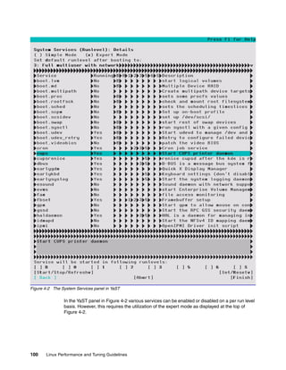
109. Chapter 4. Tuning the operating system 95
Example 4-1 Partial output from dmesg
Linux version 2.6.18-8.el5 (brewbuilder@ls20-bc1-14.build.redhat.com) (gcc version 4.1.1
20070105 (Red Hat 4.1.
1-52)) #1 SMP Fri Jan 26 14:15:14 EST 2007
Command line: ro root=/dev/VolGroup00/LogVol00 rhgb quiet
No NUMA configuration found
Faking a node at 0000000000000000-0000000140000000
Bootmem setup node 0 0000000000000000-0000000140000000
On node 0 totalpages: 1029288
DMA zone: 2726 pages, LIFO batch:0
DMA32 zone: 768002 pages, LIFO batch:31
Normal zone: 258560 pages, LIFO batch:31
Kernel command line: ro root=/dev/VolGroup00/LogVol00 rhgb quiet
Initializing CPU#0
Memory: 4042196k/5242880k available (2397k kernel code, 151492k reserved, 1222k data, 196k
init)
Calibrating delay using timer specific routine.. 7203.13 BogoMIPS (lpj=3601568)
Security Framework v1.0.0 initialized
SELinux: Initializing.
SELinux: Starting in permissive mode
CPU: Trace cache: 12K uops, L1 D cache: 16K
CPU: L2 cache: 1024K
using mwait in idle threads.
CPU: Physical Processor ID: 0
CPU: Processor Core ID: 0
CPU0: Thermal monitoring enabled (TM2)
SMP alternatives: switching to UP code
ACPI: Core revision 20060707
Using local APIC timer interrupts.
result 12500514
Detected 12.500 MHz APIC timer.
SMP alternatives: switching to SMP code
sizeof(vma)=176 bytes
sizeof(page)=56 bytes
sizeof(inode)=560 bytes
sizeof(dentry)=216 bytes
sizeof(ext3inode)=760 bytes
sizeof(buffer_head)=96 bytes
sizeof(skbuff)=240 bytes
io scheduler noop registered
io scheduler anticipatory registered
io scheduler deadline registered
io scheduler cfq registered (default)
SCSI device sda: 143372288 512-byte hdwr sectors (73407 MB)
sda: assuming Write Enabled
sda: assuming drive cache: write through
eth0: Tigon3 [partno(BCM95721) rev 4101 PHY(5750)] (PCI Express) 10/100/1000BaseT Ethernet
00:11:25:3f:19:b4
eth0: RXcsums[1] LinkChgREG[0] MIirq[0] ASF[1] Split[0] WireSpeed[1] TSOcap[1]
eth0: dma_rwctrl[76180000] dma_mask[64-bit]
EXT3 FS on dm-0, internal journal

110. 96 Linux Performance and Tuning Guidelines
kjournald starting. Commit interval 5 seconds
EXT3 FS on sda1, internal journal
EXT3-fs: mounted filesystem with ordered data mode.
ulimit
This command is built into the bash shell and is used to provide control over the resources
available to the shell and to the processes started by it on systems that allow such control.
Use the -a option to list all parameters that we can set:
ulimit -a
Example 4-2 Output of ulimit
[root@x232 html]# ulimit -a
core file size (blocks, -c) 0
data seg size (kbytes, -d) unlimited
file size (blocks, -f) unlimited
max locked memory (kbytes, -l) 4
max memory size (kbytes, -m) unlimited
open files (-n) 1024
pipe size (512 bytes, -p) 8
stack size (kbytes, -s) 10240
cpu time (seconds, -t) unlimited
max user processes (-u) 7168
virtual memory (kbytes, -v) unlimited
The -H and -S options specify the hard and soft limits that can be set for the given resource. If
the soft limit is passed, the system administrator will receive a warning. The hard limit is the
maximum value that can be reached before the user gets the error messages Out of file
handles.
For example, you can set a hard limit for the number of file handles and open files (-n):
ulimit -Hn 4096
For the soft limit of number of file handles and open files, use:
ulimit -Sn 1024
To see the hard and soft values, issue the command with a new value:
ulimit -Hn
ulimit -Sn
This command can be used, for example, to limit Oracle® users on the fly. To set it on startup,
enter the following lines, for example, in /etc/security/limits.conf:
soft nofile 4096
hard nofile 10240
In addition, make sure that the default pam configuration file (/etc/pam.d/system-auth for
Red Hat Enterprise Linux, /etc/pam.d/common-session for SUSE Linux Enterprise Server)
has the following entry:
session required pam_limits.so
This entry is required so that the system can enforce these limits.

111. Chapter 4. Tuning the operating system 97
For the complete syntax of the ulimit command, issue:
ulimit -?
4.2.3 Minimize resource use
Systems that are designed for the highest levels of performance must minimize any wasting
of resources. A race car will not offer the same amenities as a normal passenger car, but for
the purpose of driving as fast as possible cup holders and comfortable seats are a waste of
resources. The same concept is true for server systems. Running a memory consuming GUI
and a vast amount of unnecessary daemons will decrease overall performance. This section
covers the optimization of system resource consumption.
Daemons
After a default installation of Linux distributions, several possibly unnecessary services and
daemons might be enabled. Disabling unneeded daemons reduces the overall memory
footprint of the system, reduces the amount of running processes and context switches, and
more importantly, reduces exposure to various security threats. Disabling unneeded daemons
also decreases startup time of the server.
By default, several daemons that have been started can be stopped and disabled safely on
most systems. Table 4-2 lists the daemons that are started in various Linux installations. You
should consider disabling these in your environment if applicable. Note that the table lists the
respective daemons for several commercially available Linux distributions. The exact number
of running daemons might differ from your specific Linux installation. For a more detailed
explanation of these daemons, refer to the system-config-services shown in Figure 4-1 on
page 99 or the YaST GUI as displayed in Figure 4-2 on page 100.
Table 4-2 Tunable daemons started on a default installation
Daemons Description
apmd Advanced power management daemon. apmd will usually not be used on a server.
arptables_jf User space program for the arptables network filter. Unless you plan to use arptables,
you can safely disable this daemon.
autofs Automatically mounts file systems on demand (for example, mounts a CD-ROM
automatically). On server systems, file systems rarely have to be mounted
automatically.
cpuspeed Daemon to dynamically adjust the frequency of the CPU. In a server environment, this
daemon is recommended off.
cups Common UNIX Printing System. If you plan to provide print services with your server,
do not disable this service.
gpm Mouse server for the text console. Do not disable if you want mouse support for the
local text console.
hpoj HP OfficeJet support. Do not disable if you plan to use an HP OfficeJet printer with your
server.
irqbalance Balances interrupts between multiple processors. You may safely disable this daemon
on a singe CPU system or if you plan to balance IRQ statically.
isdn ISDN modem support. Do not disable if you plan to use an ISDN modem with your
server.
kudzu Detects and configures new hardware. Should be run manually in case of a hardware
change.

112. 98 Linux Performance and Tuning Guidelines
On Novell SUSE and Red Hat Enterprise Linux systems, the /sbin/chkconfig command
provides the administrator with an easy-to-use interface to change start options for various
daemons. One of the first commands that should be run when using chkconfig is a check for
all running daemons:
/sbin/chkconfig --list | grep on
If you do not want the daemon to start the next time the machine boots, issue either one of
the following commands as root. They accomplish the same results, the difference being that
the second command disables a daemon on all run levels, whereas the --level flag can be
used to specify exact run levels:
/sbin/chkconfig --levels 2345 sendmail off
/sbin/chkconfig sendmail off
There is another useful system command, /sbin/service, that enables an administrator to
immediately change the status of any registered service. In a first instance, an administrator
should always choose to check the current status of a service (sendmail in our example) by
issuing this command:
/sbin/service sendmail status
To immediately stop the sendmail daemon in our example, use this command:
netfs Used in support of exporting NFS shares. Do not disable if you plan to provide NFS
shares with your server.
nfslock Used for file locking with NFS. Do not disable if you plan to provide NFS shares with
your server.
pcmcia PCMCIA support on a server. Server systems rarely rely on a PCMCIA adapter so
disabling this daemon is safe in most instances.
portmap Dynamic port assignment for RPC services (such as NIS and NFS). If the system does
not provide RPC-based services there is no need for this daemon.
rawdevices Provides support for raw device bindings. If you do not intend to use raw devices you
may safely turn it off.
rpc* Various remote procedure call daemons mainly used for NFS and Samba. If the
system does not provide RPC-based services, there is no need for this daemon.
sendmail Mail Transport Agent. Do not disable this daemon if you plan to provide mail services
with the respective system.
smartd Self Monitor and Reporting Technology daemon that watches S.M.A.R.T. compatible
devices for errors. Unless you use an IDE/ SATA technology based disk subsystem,
there is no need for S.M.A.R.T. Monitoring.
xfs Font server for X Windows. If you will run in runlevel 5, do not disable this daemon.
Attention: Turning off the xfs daemon prevents X from starting on the server. This should
be turned off only if the server will not be booting into the GUI. Simply starting the xfs
daemon before issuing the startx command enables X to start normally.
Tip: Instead of wasting precious time waiting for a reboot to complete, simply change the
run level to 1 and back to 3 or 5, respectively.
Daemons Description

113. Chapter 4. Tuning the operating system 99
/sbin/service sendmail stop
The service command is especially useful because it lets you immediately verify whether or
not a daemon is needed. Changes performed through chkconfig will not be active unless you
change the system run level or perform a reboot. However, a daemon disabled by the service
command will be re-enabled after a reboot. Should the service command not be available
with your Linux distribution you can start or stop a daemon through the init.d directory.
Checking the status of the CUPS daemon, for example, could be performed like this:
/etc/init.d/cups status
Similarly, there are GUI-based programs for modifying which daemons are started, as shown
in Figure 4-1. To run the service configuration GUI for Red Hat Enterprise Linux, click Main
Menu → System Settings → Server Settings → Services or issue this command:
/usr/bin/redhat-config-services
Figure 4-1 Red Hat Service Configuration interface
Novell SUSE systems offer the same features via the YaST utility. In YaST the service
configuration can be found under System → System Services (Runlevel). Once in the
service configuration we suggest you use the expert mode in order to accurately set the
status of the respective daemon. Running YaST in runlevel 3 would look as shown in
Figure 4-2 on page 100.
To change the current state,
highlight the daemon and
click Stop.
The check mark indicates the
daemon will start at the next
reboot.

114. 100 Linux Performance and Tuning Guidelines
Figure 4-2 The System Services panel in YaST
In the YaST panel in Figure 4-2 various services can be enabled or disabled on a per run level
basis. However, this requires the utilization of the expert mode as displayed at the top of
Figure 4-2.

115. Chapter 4. Tuning the operating system 101
Changing runlevels
Whenever possible, do not run the graphical user interface on a Linux server. Normally, there
is no need for a GUI on a Linux server, as most Linux administrators will happily assure you.
All administrative tasks can be achieved efficiently through the command line, by redirecting
the X display, or through a Web browser interface. If you prefer a graphical interface, there are
several useful Web based tools such as webmin, Linuxconf, and SWAT.
If a GUI must be used, start and stop it as needed rather than running it all the time. In most
cases the server should be running at runlevel 3, which does not start the X Server when the
machine boots up. If you want to restart the X Server, use startx from a command prompt.
1. Determine which run level the machine is running by using the runlevel command.
This prints the previous and current run level. For example, N 5 means that there was no
previous run level (N) and that the current run level is 5.
2. To switch between run levels, use the init command. For example, to switch to runlevel 3,
enter the init 3 command.
The run levels that are used in Linux are:
0 Halt (Do not set initdefault to this or the server will shut down immediately after
finishing the boot process.)
1 Single user mode
2 Multiuser, without NFS (the same as 3 if you do not have networking)
3 Full multiuser mode
4 Unused
5 X11
6 Reboot (Do not set initdefault to this or the server machine will continuously reboot
at startup.)
To set the initial runlevel of a machine at boot, modify the /etc/inittab file as shown in
Figure 4-3 on page 102 with the line:
id:3:initdefault:
Tip: Even if the GUI is disabled locally on the server, you can still connect remotely and
use the GUI. To do this, use the -X parameter with the ssh command.

116. 102 Linux Performance and Tuning Guidelines
Figure 4-3 /etc/inittab, modified (only part of the file is displayed)
Limiting local terminals
By default, several virtual consoles are spawned locally. The amount of memory used by the
virtual terminals is negligible; nevertheless we try to get the most out of any system.
Troubleshooting and process analysis will be simplified by simply reducing the amount of
running processes, which is the reason for limiting the local terminals to two.
To do this, comment out each mingetty ttyx line you want to disable. As an example, in
Figure 4-3 we limited the consoles to two. This gives you a fallback local terminal in case a
command kills the shell you were working on locally.
4.2.4 SELinux
Red Hat Enterprise Linux 4 introduced a new security model, Security Enhanced Linux
(SELinux), which is a significant step towards higher security. SELinux introduces a
... (lines not displayed)
# The default runlevel is defined here
id:3:initdefault:
# First script to be executed, if not booting in emergency (-b) mode
si::bootwait:/etc/init.d/boot
# /etc/init.d/rc takes care of runlevel handling
#
# runlevel 0 is System halt (Do not use this for initdefault!)
# runlevel 1 is Single user mode
# runlevel 2 is Local multiuser without remote network (e.g. NFS)
# runlevel 3 is Full multiuser with network
# runlevel 4 is Not used
# runlevel 5 is Full multiuser with network and xdm
# runlevel 6 is System reboot (Do not use this for initdefault!)
#
... (lines not displayed)
# getty-programs for the normal runlevels
# <id>:<runlevels>:<action>:<process>
# The “id” field MUST be the same as the last
# characters of the device (after “tty”).
1:2345:respawn:/sbin/mingetty --noclear tty1
2:2345:respawn:/sbin/mingetty tty2
#3:2345:respawn:/sbin/mingetty tty3
#4:2345:respawn:/sbin/mingetty tty4
#5:2345:respawn:/sbin/mingetty tty5
#6:2345:respawn:/sbin/mingetty tty6
#
#S0:12345:respawn:/sbin/agetty -L 9600 ttyS0 vt102
... (lines not displayed)
To start Linux without starting
the GUI, set the run level to 3.
To only provide two local
virtual terminals, comment
out the mingetty entries for
3, 4, 5, and 6.

117. Chapter 4. Tuning the operating system 103
mandatory policy model that overcomes the limitations of the standard discretionary access
model employed by Linux. SELinux enforces security on user and process levels; so a
security flaw of any given process affects only the resources allocated to this process and not
the entire system. SELinux works like a virtual machine. For example, if a malicious attacker
uses a root exploit within Apache, only the resources allocated to the Apache daemon could
be compromised.
Figure 4-4 Schematic overview of SELinux
However, enforcing such a policy based security model comes at a price. Every access from
a user or process to a system resource such as an I/O device must be controlled by SELinux.
The process of checking permissions can cause overhead of up to 10%. SELinux is of great
value to any edge server such as a firewall or a Web server, but the added level of security on
a back-end database server might not justify the loss in performance.
Generally, the easiest way to disable SELinux is to not install it in the first place. But often
systems have been installed using default parameters, unaware that SELinux affects
performance. To disable SELinux after an installation, append the entry selinux=0 to the line
containing the running kernel in the GRUB boot loader (Example 4-3).
Example 4-3 Sample grub.conf file with disabled SELinux
default=0
splashimage=(hd0,0)/grub/splash.xpm.gz
hiddenmenu
title Red Hat Enterprise Linux AS (2.6.9-5.ELsmp)
root (hd0,0)
kernel /vmlinuz-2.6.9-5.ELsmp ro root=LABEL=/ selinux=0
initrd /initrd-2.6.9-5.ELsmp.img
Another way of disabling SELinux is through the SELinux configuration file stored under
/etc/selinux/config. Disabling SELinux from within that file looks as shown in Example 4-4.
Example 4-4 Disabling SELinux via the config file
# This file controls the state of SELinux on the system.
# SELINUX= can take one of these three values:
# enforcing - SELinux security policy is enforced.
# permissive - SELinux prints warnings instead of enforcing.
# disabled - SELinux is fully disabled.
SELinux Kernel
SECURITY
POLICY
SECURITY
ENFORCEMENT
MODULE
Process
User
SYSTEM
RESOURCES
Request
Access
Grant
Access
Grant/Deny Access
Based on Policy

118. 104 Linux Performance and Tuning Guidelines
SELINUX=disabled
# SELINUXTYPE= type of policy in use. Possible values are:
# targeted - Only targeted network daemons are protected.
# strict - Full SELinux protection.
SELINUXTYPE=targeted
If you decide to use SELinux with your Linux-based server, its settings can be tweaked to
better accommodate your environment. On a running system, check whether the working set
of the cached Linux Security Modules (LSM) permissions exceeds the default Access Vector
Cache (AVC) size of 512 entries.
Check /selinux/avc/hash_stats for the length of the longest chain. Anything over 10 signals
a likely bottleneck.
If the system experiences a bottleneck in the Access Vector Cache (for example, on a heavily
loaded firewall), try to resize /selinux/avc/cache_threshold to a slightly higher value and
recheck the hash stats.
4.2.5 Compiling the kernel
Creating and compiling your own kernel has far less of an impact on improving system
performance than often thought. Modern kernels shipped with most Linux distributions are
modular—they load only the parts that are used. Recompiling the kernel can decrease kernel
size and its overall behavior (for example, real-time behavior). Changing certain parameters
in the source code might also yield some system performance. However, non-standard
kernels are not covered in the support subscription that is provided with most Enterprise
Linux distributions. Additionally, the extensive ISV application and IBM hardware certifications
that are provided for Enterprise Linux distributions are nullified if a non-standard kernel is
used.
Having said that, performance improvements can be gained with a custom made kernel, but
they hardly justify the challenges you face running an unsupported kernel in an enterprise
environment. While this is true for commercial workloads, if scientific workloads such as high
performance computing are your area of interest, custom kernels might be of interest to you.
Do not attempt to use special compiler flags such as -C09 when recompiling the kernel. The
source code for the Linux kernel has been hand tuned to match the GNU C compiler. Using
special compiler flags might at best decrease the kernel performance and at worst break the
code.
Keep in mind that unless you really know what you are doing, you might actually decrease
system performance due to wrong kernel parameters.
4.3 Changing kernel parameters
Although modifying and recompiling the kernel source code is not recommended for most
users, the Linux kernel features yet another means of tweaking kernel parameters. The proc
file system provides an interface to the running kernel that can be used for monitoring
purposes and for changing kernel settings on the fly.
Tip: To check for usage statistics of the access vector cache you may alternatively use the
avcstat utility.

119. Chapter 4. Tuning the operating system 105
To view the current kernel configuration, choose a kernel parameter in the /proc/sys
directory and use the cat command on the respective file. In Example 4-5 we parse the
system for its current memory overcommit strategy. The output 0 tells us that the system will
always check for available memory before granting an application a memory allocation
request. To change this default behavior we can use the echo command and supply it with the
new value, 1 in the case of our example (1 meaning that the kernel will grant every memory
allocation without checking whether the allocation can be satisfied).
Example 4-5 Changing kernel parameters via the proc file system
[root@linux vm]# cat overcommit_memory
0
[root@linux vm]# echo 1 > overcommit_memory
While the demonstrated way of using cat and echo to change kernel parameters is fast and
available on any system with the proc file system, it has two significant shortcomings.
򐂰 The echo command does not perform any consistency check on the parameters.
򐂰 All changes to the kernel are lost after a reboot of the system.
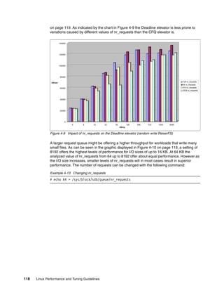
To overcome this, a utility called sysctl aids the administrator in changing kernel parameters.
In addition, Red Hat Enterprise Linux and Novell SUSE Enterprise Linux offer graphical
methods of modifying these sysctl parameters. Figure 4-5 shows one of the user interfaces.
Figure 4-5 Red Hat kernel tuning
Tip: By default, the kernel includes the necessary module to enable you to make changes
using sysctl without having to reboot. However, If you chose to remove this support
(during the operating system installation), then you will have to reboot Linux before the
change will take effect.

120. 106 Linux Performance and Tuning Guidelines
For Novell SUSE based systems, YaST and more specifically powertweak is the tool of choice
for changing any kernel parameter.
Figure 4-6 The powertweak utility
The big advantage of powertweak through sysctl is that all tuning parameters are presented
with a short explanation. Note that all changes made with the help of powertweak will be
stored under /etc/powertweak/tweaks.
4.3.1 Where the parameters are stored
The kernel parameters that control how the kernel behaves are stored in /proc (in particular,
/proc/sys).
Reading the files in the /proc directory tree provides a simple way to view configuration
parameters that are related to the kernel, processes, memory, network, and other
components. Each process running in the system has a directory in /proc with the process ID
(PID) as its name. Table 4-3 on page 107 lists some of the files that contain kernel
information.

121. Chapter 4. Tuning the operating system 107
Table 4-3 Parameter files in /proc
4.3.2 Using the sysctl command
The sysctl command uses the names of files in the /proc/sys directory tree as parameters.
For example, to modify the shmmax kernel parameter, you can display (using cat) and
change (using echo) the file /proc/sys/kernel/shmmax:
#cat /proc/sys/kernel/shmmax
33554432
#echo 33554430 > /proc/sys/kernel/shmmax
#cat /proc/sys/kernel/shmmax
33554430
However, using these commands can easily introduce errors, so we recommend that you use
the sysctl command because it checks the consistency of the data before it makes any
change. For example:
#sysctl kernel.shmmax
kernel.shmmax = 33554432
#sysctl -w kernel.shmmax=33554430
kernel.shmmax = 33554430
#sysctl kernel.shmmax
kernel.shmmax = 33554430
This change to the kernel stays in effect only until the next reboot. If you want to make the
change permanently, then you can edit the /etc/sysctl.conf file and add the appropriate
command. In our example:
kernel.shmmax = 33554439
The next time you reboot, the parameter file will be read. You can do the same thing without
rebooting by issuing the following command:
#sysctl -p
4.4 Tuning the processor subsystem
In any computer, whether it is a hand held device or a cluster for scientific applications, the
main subsystem is the processor that does the actual computing. During the past decade
Moore’s Law has caused processor subsystems to evolve significantly faster than other
subsystems. The result is that bottlenecks rarely occur within the CPU, unless number
crunching is the sole purpose of the system. This is illustrated by the average CPU utilization
of an Intel compatible server system that lies below 10%. It is important to understand the
File/directory Purpose
/proc/sys/abi/* Used to provide support for “foreign” binaries, not native to Linux — those
compiled under other UNIX variants such as SCO UnixWare 7, SCO
OpenServer, and SUN Solaris™ 2. By default, this support is installed,
although it can be removed during installation.
/proc/sys/fs/* Used to increase the number of open files the OS allows and to handle quota.
/proc/sys/kernel/* For tuning purposes, you can enable hotplug, manipulate shared memory, and
specify the maximum number of PID files and level of debug in syslog.
/proc/sys/net/* Tuning of network in general, IPV4 and IPV6.
/proc/sys/vm/* Management of cache memory and buffer.

122. 108 Linux Performance and Tuning Guidelines
bottlenecks that can occur at the processor level and to know possible tuning parameters in
order to improve CPU performance.
4.4.1 Tuning process priority
As we stated in 1.1.4, “Process priority and nice level” on page 5, it is not possible to change
the process priority of a process. This is only indirectly possible through the use of the nice
level of the process, but even this is not always possible. If a process is running too slowly,
you can assign more CPU to it by giving it a lower nice level. Of course, this means that all
other programs will have fewer processor cycles and will run more slowly.
Linux supports nice levels from 19 (lowest priority) to -20 (highest priority). The default value
is 0. To change the nice level of a program to a negative number (which makes it higher
priority), it is necessary to log on or su to root.
To start the program xyz with a nice level of -5, issue the command:
nice -n -5 xyz
To change the nice level of a program already running, issue the command:
renice level pid
To change the priority of a program with a PID of 2500 to a nice level of 10, issue:
renice 10 2500
4.4.2 CPU affinity for interrupt handling
Two principles have proven to be most efficient when it comes to interrupt handling (refer to
1.1.6, “Interrupt handling” on page 6 for a review of interrupt handling):
򐂰 Bind processes that cause a significant amount of interrupts to a CPU.
CPU affinity enables the system administrator to bind interrupts to a group or a single
physical processor (of course, this does not apply on a single CPU system). To change the
affinity of any given IRQ, go into /proc/irq/%{number of respective irq}/ and change
the CPU mask stored in the file smp_affinity. To set the affinity of IRQ 19 to the third CPU
in a system (without SMT) use the command in Example 4-6.
Example 4-6 Setting the CPU affinity for interrupts
[root@linux /]#echo 03 > /proc/irq/19/smp_affinity
򐂰 Let physical processors handle interrupts.
In symmetric multi-threading (SMT) systems such as IBM POWER 5+ processors
supporting multi-threading, it is suggested that you bind interrupt handling to the physical
processor rather than the SMT instance. The physical processors usually have the lower
CPU numbering so in a two-way system with multi-threading enabled, CPU ID 0 and 2
would refer to the physical CPU, and 1 and 3 would refer to the multi-threading instances.
If you do not use the smp_affinity flag, you will not have to worry about this.
4.4.3 Considerations for NUMA systems
Non-Uniform Memory Architecture (NUMA) systems are gaining market share and are seen
as the natural evolution of classic symmetric multiprocessor systems. Although the CPU
scheduler used by current Linux distributions is well suited for NUMA systems, applications
might not always be. Bottlenecks caused by a non-NUMA aware application can cause

123. Chapter 4. Tuning the operating system 109
performance degradations that are hard to identify. The recent numastat utility shipped in the
numactl package helps to identify processes that have difficulties dealing with NUMA
architectures.
To help with spotting bottlenecks, statistics provided by the numastat tool are available in the
/sys/devices/system/node/%{node number}/numastat file. High values in numa_miss and
the other_node field signal a likely NUMA issue. If you find that a process is allocated memory
that does not reside on the local node for the process (the node that holds the processors that
run the application), try to renice the process to the other node or work with NUMA affinity.
4.5 Tuning the vm subsystem
Tuning the memory subsystem is a challenging task that requires constant monitoring to
ensure that changes do not negatively affect other subsystems in the server. If you do choose
to modify the virtual memory parameters (in /proc/sys/vm), we recommend that you change
only one parameter at a time and monitor how the server performs.
Remember that most applications under Linux do not write directly to the disk; they write to
the file system cache maintained by the virtual memory manager that will eventually flush out
the data. When using an IBM ServeRAID controller or an IBM TotalStorage disk subsystem,
you should try to the decrease the number of flushes, effectively increasing the I/O stream
caused by each flush. The high-performance disk controller can handle the larger I/O stream
more efficiently than multiple small ones.
4.5.1 Setting kernel swap and pdflush behavior
With the introduction of the improved virtual memory subsystem in the Linux kernel 2.6,
administrators now have a simple interface to fine-tune the swapping behavior of the kernel.
򐂰 The parameter stored in /proc/sys/vm/swappiness can be used to define how
aggressively memory pages are swapped to disk. An introduction to the Linux virtual
memory manager and the general use of swap space in Linux is discussed in “Page frame
reclaiming” on page 14. It states that Linux moves memory pages that have not been
accessed for some time to the swap space even if there is enough free memory available.
By changing the percentage in /proc/sys/vm/swappiness you can control that behavior,
depending on the system configuration. If swapping is not desired,
/proc/sys/vm/swappiness should have low values. Systems with memory constraints that
run batch jobs (processes that sleep for a long time) might benefit from an aggressive
swapping behavior. To change swapping behavior, use either echo or sysctl as shown in
Example 4-7.
Example 4-7 Changing swappiness behavior
# sysctl -w vm.swappiness=100
򐂰 Especially for fast disk subsystems, it might also be desirable to cause large flushes of
dirty memory pages. The value stored in /proc/sys/vm/dirty_background_ratio defines
at what percentage of main memory the pdflush daemon should write data out to the disk.
If larger flushes are desired then increasing the default value of 10% to a larger value will
cause less frequent flushes. As in the example above, the value can be changed as shown
in Example 4-8.
Example 4-8 Increasing the wake up time of pdflush
# sysctl -w vm.dirty_background_ratio=25

124. 110 Linux Performance and Tuning Guidelines
򐂰 Another related setting in the virtual memory subsystem is the ratio at which dirty pages
created by application disk writes will be flushed out to disk. As explained in chapter one
1.3.1, “Virtual file system” on page 15, writes to the file system will not be written instantly
but rather written in the page cache and flushed out to the disk subsystem at a later stage.
Using the parameter stored in /proc/sys/vm/dirty_ratio the system administrator can
define at what level the actual disk writes will take place. The value stored in dirty_ratio
is a percentage of main memory. A value of 10 would mean that data will be written into
system memory until the file system cache has a size of 10% of the server’s RAM. As in
the previous two examples, the ratio at which dirty pages are written to disk can be altered
as follows to a setting of 20% of the system memory:
Example 4-9 Altering the dirty ratio
# sysctl -w vm.dirty_ratio=20
4.5.2 Swap partition
The swap device is used when physical RAM is fully in use and the system needs additional
memory. Linux also uses swap space to page memory areas to disk that have not been
accessed for a significant amount of time. When no free memory is available on the system, it
begins paging the least used data from memory to the swap areas on the disks. The initial
swap partition is created during the Linux installation process with current guidelines stating
that the size of the swap partition should be two times physical RAM. Linux kernels 2.4 and
beyond support swap sizes up to 24 GB per partition with an 8 TB theoretical maximum for
32-bit systems. Swap partitions should reside on separate disks.
If more memory is added to the server after the initial installation, additional swap space must
be configured. There are two ways to configure additional swap space after the initial install:
򐂰 A free partition on the disk can be created as a swap partition. This can be difficult if the
disk subsystem has no free space available. In that case, a swap file can be created.
򐂰 If there is a choice, the preferred option is to create additional swap partitions. There is a
performance benefit because I/O to the swap partitions bypasses the file system and all of
the overhead involved in writing to a file.
Another way to improve the performance of swap partitions and files is to create multiple swap
partitions. Linux can take advantage of multiple swap partitions or files and perform the reads
and writes in parallel to the disks. After creating the additional swap partitions or files, the
/etc/fstab file will contain such entries as those shown in Example 4-10.
Example 4-10 /etc/fstab file
/dev/sda2 swap swap sw 0 0
/dev/sdb2 swap swap sw 0 0
/dev/sdc2 swap swap sw 0 0
/dev/sdd2 swap swap sw 0 0
Under normal circumstances, Linux would use the /dev/sda2 swap partition first, then
/dev/sdb2, and so on, until it had allocated enough swapping space. This means that perhaps
only the first partition, /dev/sda2, will be used if there is no need for a large swap space.
Spreading the data over all available swap partitions improves performance because all
read/write requests are performed simultaneously to all selected partitions. Changing the file
as shown in Example 4-11 on page 111 assigns a higher priority level to the first three
partitions.

125. Chapter 4. Tuning the operating system 111
Example 4-11 Modified /ertc/fstab to make parallel swap partitions
/dev/sda2 swap swap sw,pri=3 0 0
/dev/sdb2 swap swap sw,pri=3 0 0
/dev/sdc2 swap swap sw,pri=3 0 0
/dev/sdd2 swap swap sw,pri=1 0 0
Swap partitions are used from the highest priority to the lowest (where 32767 is the highest
and 0 is the lowest). Giving the same priority to the first three disks causes the data to be
written to all three disks; the system does not wait until the first swap partition is full before it
starts to write on the next partition. The system uses the first three partitions in parallel and
performance generally improves.
The fourth partition is used if additional space is needed for swapping after the first three are
completely filled up. It is also possible to give all partitions the same priority to stripe the data
over all partitions, but if one drive is slower than the others, performance would decrease. A
general rule is that the swap partitions should be on the fastest drives available.
4.5.3 HugeTLBfs
This memory management feature is valuable for applications that use a large virtual address
space. It is especially useful for database applications.
The CPU’s Translation Lookaside Buffer (TLB) is a small cache used for storing virtual-to-
physical mapping information. By using the TLB, a translation can be performed without
referencing the in-memory page table entry that maps the virtual address. However, to keep
translations as fast as possible, the TLB is usually small. It is not uncommon for large memory
applications to exceed the mapping capacity of the TLB.
The HugeTLBfs feature permits an application to use a much larger page size than normal,
so that a single TLB entry can map a larger address space. A HugeTLB entry can vary in
size. For example, in an Itanium® 2 system, a huge page might be 1000 times larger than a
normal page. This enables the TLB to map 1000 times the virtual address space of a normal
process without incurring a TLB cache miss. For simplicity, this feature is exposed to
applications by means of a file system interface.
To allocate hugepage, you can define the number of hugepages by configuring value at
/proc/sys/vm/nr_hugepages using sysctl command.
sysctl -w vm.nr_hugepages=512
If your application uses huge pages through the mmap() system call, you have to mount a file
system of type hugetlbfs like this:
mount -t hugetlbfs none /mnt/hugepages
/proc/meminfo file will provide information about hugetlb pages as shown in Example 4-12 on
page 112.
Important: Although there are good tools to tune the memory subsystem, frequent page
outs should be avoided as much as possible. The swap space is not a replacement for
RAM because it is stored on physical drives that have a significantly slower access time
than memory. So, frequent page out (or swap out) is almost never a good behavior. Before
trying to improve the swap process, ensure that your server has enough memory or that
there is no memory leak.

126. 112 Linux Performance and Tuning Guidelines
Example 4-12 Hugepage information in /proc/meminfo
[root@lnxsu4 ~]# cat /proc/meminfo
MemTotal: 4037420 kB
MemFree: 386664 kB
Buffers: 60596 kB
Cached: 238264 kB
SwapCached: 0 kB
Active: 364732 kB
Inactive: 53908 kB
HighTotal: 0 kB
HighFree: 0 kB
LowTotal: 4037420 kB
LowFree: 386664 kB
SwapTotal: 2031608 kB
SwapFree: 2031608 kB
Dirty: 0 kB
Writeback: 0 kB
Mapped: 148620 kB
Slab: 24820 kB
CommitLimit: 2455948 kB
Committed_AS: 166644 kB
PageTables: 2204 kB
VmallocTotal: 536870911 kB
VmallocUsed: 263444 kB
VmallocChunk: 536607255 kB
HugePages_Total: 1557
HugePages_Free: 1557
Hugepagesize: 2048 kB
Please refer to kernel documentation in Documentation/vm/hugetlbpage.txt for more
information.
4.6 Tuning the disk subsystem
Ultimately, all data must be retrieved from and stored to disk. Disk accesses are usually
measured in milliseconds and are at least thousands of times slower than other components
(such as memory and PCI operations, which are measured in nanoseconds or
microseconds). The Linux file system is the method by which data is stored and managed on
the disks.
Many different file systems are available for Linux that differ in performance and scalability.
Besides storing and managing data on the disks, file systems are also responsible for
guaranteeing data integrity. The newer Linux distributions include journaling file systems as
part of their default installation. Journaling, or logging, prevents data inconsistency in case of
a system crash. All modifications to the file system metadata have been maintained in a
separate journal or log and can be applied after a system crash to bring it back to its
consistent state. Journaling also improves recovery time, because there is no need to perform
file system checks at system reboot. As with other aspects of computing, you will find that
there is a trade-off between performance and integrity. However, as Linux servers make their
way into corporate data centers and enterprise environments, requirements such as high
availability can be addressed.

127. Chapter 4. Tuning the operating system 113
In addition to the various file systems, the Linux kernel 2.6 knows 4 distinct I/O scheduling
algorithms that again can be used to tailor the system to a specific task. Each I/O elevator has
distinct features that might or might not make it suitable for a specific hardware configuration
and a desired task. While some elevators pronounce streaming I/O as it is often found in
multimedia or desktop PC environments, other elevators focus on low latency access times
necessary for database workloads.
In this section we cover the characteristics and tuning options of the standard file system such
as ReiserFS and Ext3 and the tuning potential found in the kernel 2.6 I/O elevators.
4.6.1 Hardware considerations before installing Linux
Minimum requirements for CPU speed and memory are well documented for current Linux
distributions. Those instructions also provide guidance for the minimum disk space that is
required to complete the installation. However, they fall short on explaining how to initially set
up the disk subsystem. Linux servers cover a vast assortment of work environments, because
server consolidation impacts data centers. One of the first questions to answer is: What is the
function of the server being installed?
A server’s disk subsystems can be a major component of overall system performance.
Understanding the function of the server is key to determining whether the I/O subsystem will
have a direct impact on performance.
Examples of servers where disk I/O is the most important subsystem:
򐂰 A file and print server must move data quickly between users and disk subsystems.
Because the purpose of a file server is to deliver files to the client, the server must initially
read all data from a disk.
򐂰 A database server’s ultimate goal is to search and retrieve data from a repository on the
disk. Even with sufficient memory, most database servers perform large amounts of disk
I/O to bring data records into memory and flush modified data to disk.
Examples of servers where disk I/O is not the most important subsystem:
򐂰 An e-mail server acts as a repository and router for electronic mail and tends to generate a
heavy communication load. Networking is more important for this type of server.
򐂰 A Web server that is responsible for hosting Web pages (static, dynamic, or both) benefits
from a well tuned network and memory subsystem.
Number of drives
The number of disk drives significantly affects performance because each drive contributes to
total system throughput. Capacity requirements are often the only consideration used to
determine the number of disk drives that are configured in a server. Throughput requirements
are usually not well understood or are completely ignored. The key to a well performing disk
subsystem is maximizing the number of read-write heads that can service I/O requests.
With RAID (redundant array of independent disks) technology, you can spread the I/O over
multiple spindles. There are two options for implementing RAID in a Linux environment:
software RAID and hardware RAID. Unless your server hardware comes standard with
hardware RAID, you might want to start with the software RAID options that come with the
Linux distributions. If a need arises, you can grow into the more efficient hardware RAID
solutions.
If it is necessary to implement a hardware RAID array, you will need a RAID controller for your
system. In this case the disk subsystem consists of the physical hard disks and the controller.

128. 114 Linux Performance and Tuning Guidelines
It is paramount to remember that the disk subsystem performance ultimately depends on the
number of input output requests a given device is able to handle. Once the operating system
cache and the cache of the disk subsystem can no longer accommodate the amount or size
of a read or write request, the physical disk spindles have to work. Consider the following
example. A disk device is able to handle 200 I/Os per second. You have an application that
performs 4 KB write requests at random locations on the file systems so streaming or request
merging is not an option. The maximum throughput of the specified disk subsystem is now:
I/Os per second of physical disk * request size = maximum throughput
Hence the example above results in:
200 * 4 KB = 800 KB
Since the 800 KB is a physical maximum, the only possibility to improve performance in this
case is to either add more spindles or physical disks or to cause the application to write larger
I/Os. Databases such as DB2 can be configured to use larger request sizes that will in most
cases improve disk throughput.
For more information on available IBM storage solutions, see:
򐂰 IBM System Storage Solutions Handbook, SG24-5250
򐂰 Introduction to Storage Area Networks, SG24-5470
Guidelines for setting up partitions
A partition is a contiguous set of blocks on a drive that are treated as if they were independent
disks. The default installation of today’s Enterprise Linux distributions use flexible partitioning
layouts by creating one or more logical volumes.
There is a great deal of debate in Linux circles about the optimal disk partition. A single root
partition method could lead to problems in the future if you decide to redefine the partitions
because of new or updated requirements. On the other hand, too many partitions can lead to
a file system management problem. During the installation process, Linux distributions enable
you to create a multipartition layout.
There are benefits to running Linux on a multipartitioned or even logical volume disk:
򐂰 Improved security with finer granularity on file system attributes.
For example, the /var and /tmp partitions are created with attributes that permit very easy
access for all users and processes on the system and are susceptible to malicious access.
By isolating these partitions to separate disks, you can reduce the impact on system
availability if these partitions have to be rebuilt or recovered.
򐂰 Improved data integrity, so loss of data with a disk crash would be isolated to the affected
partition.
For example, if there is no RAID implementation on the system (software or hardware) and
the server suffers a disk crash, only the partitions on that bad disk would have to be
repaired or recovered.
򐂰 New installations and upgrades can be done without affecting other more static partitions.
For example, if the /home file system has not been separated to another partition, it will be
overwritten during an OS upgrade, losing all user files stored on it.
Tip: In general, adding drives is one of the most effective changes that can be made to
improve server performance.

129. Chapter 4. Tuning the operating system 115
򐂰 More efficient backup process
Partition layouts must be designed with backup tools in mind. It is important to understand
whether backup tools operate on partition boundaries or on a more granular level like file
systems.
Table 4-4 lists some of the partitions that you might want to consider separating out from root
to provide more flexibility and better performance in your environment.
Table 4-4 Linux partitions and server environments
For a more detailed look at how Linux distributions handle file system standards, see the
Filesystem Hierarchy Standard’s home page at:
http://www.pathname.com/fhs
4.6.2 I/O elevator tuning and selection
With Linux kernel 2.6 new I/O scheduling algorithms were introduced in order to allow for
more flexibility when handling different I/O patterns. A system administrator now has to select
the best suited elevator for a given hardware and software layout. Additionally each I/O
elevator features a set of tuning options to further tailor a system towards a specific workload.
Selecting the right I/O elevator in kernel 2.6
For most server workloads, either the Complete Fair Queuing (CFQ) elevator or the deadline
elevator are an adequate choice as they are optimized for the multiuser, multiprocess
environment that a typical server operates in. Enterprise distributions typically default to the
CFQ elevator. However on Linux for IBM System z, the deadline scheduler is favored as the
default elevator. Certain environments can benefit from selecting a different I/O elevator. With
Red Hat Enterprise Linux 5.0 and Novell SUSE Linux Enterprise Server 10 the I/O schedulers
can now be selected on a per disk subsystem basis as opposed to the global setting in Red
Partition Contents and possible server environments
/home A file server environment would benefit from separating out /home to its own
partition. This is the home directory for all users on the system, if there are no disk
quotas implemented, so separating this directory should isolate a user’s runaway
consumption of disk space.
/tmp If you are running a high-performance computing environment, large amounts of
temporary space are needed during compute time, then released upon completion.
/usr This is where the kernel source tree and Linux documentation (as well as most
executable binaries) are located. The /usr/local directory stores the executables that
must be accessed by all users on the system and is a good location to store custom
scripts developed for your environment. If it is separated to its own partition, then
files will not have to be reinstalled during an upgrade or reinstall by simply choosing
not to have the partition reformatted.
/var The /var partition is important in mail, Web, and print server environments because
it contains the log files for these environments and the overall system log. Chronic
messages can flood and fill this partition. If this occurs and the partition is not
separate from the /, service interruptions are possible. Depending on the
environment, further separation of this partition is possible by separating out
/var/spool/mail for a mail server or /var/log for system logs.
/opt The installation of some third-party software products, such as Oracle’s database
server, default to this partition. If not separate, the installation will continue under /
and, if there is not enough space allocated, could fail.

130. 116 Linux Performance and Tuning Guidelines
Hat Enterprise Linux 4.0 and Novell SUSE Linux Enterprise Server 9. With the possibility of
different I/O elevators per disk subsystem, the administrator now has the possibility to isolate
a specific I/O pattern on a disk subsystem (such as write intensive workloads) and select the
appropriate elevator algorithm.
򐂰 Synchronous file system access
Certain types of applications need to perform file system operations synchronously. This
can be true for databases that might even use a raw file system or for very large disk
subsystems where caching asynchronous disk accesses simply is not an option. In those
cases the performance of the anticipatory elevator usually has the least throughput and
the highest latency. The three other schedulers perform equally good up to an I/O size of
roughly 16 KB where the CFQ and the NOOP elevator begin to outperfom the deadline
elevator (unless disk access is very seek intense) as can be seen in Figure 4-7.
Figure 4-7 Random read performance per I/O elevator (synchronous)
򐂰 Complex disk subsystems
Benchmarks have shown that the NOOP elevator is an interesting alternative in high-end
server environments. When using very complex configurations of IBM ServeRAID or
TotalStorage® DS class disk subsystems, the lack of ordering capability of the NOOP
elevator becomes its strength. Enterprise class disk subsystems could contain multiple
SCSI or FibreChannel disks that each have individual disk heads and data striped across
the disks. It becomes be very difficult for an I/O elevator to anticipate the I/O
characteristics of such complex subsystems correctly, so you might often observe at least
equal performance at less overhead when using the NOOP I/O elevator. Most large scale
benchmarks that use hundreds of disks most likely use the NOOP elevator.
򐂰 Database systems
Due to the seek-oriented nature of most database workloads some performance gain can
be achieved when selecting the deadline elevator for these workloads.
򐂰 Virtual machines
Virtual machines, regardless of whether in VMware or VM for System z, usually
communicate through a virtualization layer with the underlying hardware. So, a virtual
0
20000
40000
60000
80000
100000
120000
140000
160000
180000
kB/sec
4 8 16 32 64 128 256 512 1024 2048
kB/op
Deadline
Anticipatory
CFQ
NOOP

131. Chapter 4. Tuning the operating system 117
machine is not aware of whether the assigned disk device consists of a single SCSI device
or an array of FibreChannel disks on a TotalStorage DS8000™. The virtualization layer
takes care of necessary I/O reordering and the communication with the physical block
devices.
򐂰 CPU bound applications
While some I/O schedulers can offer superior throughput they could at the same time
create more system overhead. The overhead that for instance the CFQ or deadline
elevators cause comes from aggressively merging and reordering the I/O queue.
Sometimes the workload is not so much limited by the performance of the disk subsystem
as by the performance of the CPU. Such a case could occur with a scientific workload or a
data warehouse processing very complex queries. In such scenarios the NOOP elevator
offers some advantage over the other elevators because it causes less CPU overhead as
shown on the following chart. However it should also be noted that when comparing CPU
overhead to throughput the deadline and CFQ elevators are still the best choices for most
access patterns to asynchronous file systems.
Figure 4-8 CPU utilization by I/O elevator (asynchronous)
򐂰 Single ATA or SATA disk subsystems
If you choose to use a single physical ATA or SATA disk, consider using the anticipatory
I/O elevator, which reorders disk writes to accommodate the single disk head found in
these devices.
Impact of nr_requests
The plugable I/O scheduler implementation of kernel 2.6 also features a way to increase or
decrease the number of requests that can be issued to a disk subsystem. With nr_requests,
as with so many other tuning parameters, there is no one best setting. The correct value that
should be used for the number of requests largely depends on the underlying disk subsystem
and even more on the I/O characteristics of the workload. The impact of different values of
nr_requests can also differ from the file system and I/O scheduler that you plan to use as can
be easily seen by the two benchmarks displayed in Figure 4-9 on page 118 and Figure 4-10
0
5
10
15
20
25
30
35
40
45
50
CPU%
4 8 16 32 64 128 256 512 1024 2048
kB/op
NOOP
Deadline
CFQ
Anticipatory

132. 118 Linux Performance and Tuning Guidelines
on page 119. As indicated by the chart in Figure 4-9 the Deadline elevator is less prone to
variations caused by different values of nr_requests than the CFQ elevator is.
Figure 4-9 Impact of nr_requests on the Deadline elevator (random write ReiserFS)
A larger request queue might be offering a higher throughput for workloads that write many
small files. As can be seen in the graphic displayed in Figure 4-10 on page 119, a setting of
8192 offers the highest levels of performance for I/O sizes of up to 16 KB. At 64 KB the
analyzed value of nr_requests from 64 up to 8192 offer about equal performance. However as
the I/O size increases, smaller levels of nr_requests will in most cases result in superior
performance. The number of requests can be changed with the following command:
Example 4-13 Changing nr_requests
# echo 64 > /sys/block/sdb/queue/nr_requests
0
20000
40000
60000
80000
100000
120000
140000
kB/sec
4 8 16 32 64 128 256 512 1024 2048
kB/op
128 nr_requests
64 nr_requests
512 nr_requests
2028 nr_requests

133. Chapter 4. Tuning the operating system 119
I
Figure 4-10 Impact of nr_requests on the CFQ elevator (random write Ext3)
It is important to point out that the current enterprise distributions from Red Hat and Linux
offer the option to set nr_requests on a per disk subsystem basis. So, I/O access patterns can
be isolated and optimally tuned. An example would be a database system where the log
partitions and the database would be stored on dedicated disks or disk subsystems (such as
a storage partition on a DS8300). In this example it would be beneficial to use a large
nr_reuests for the log partition that has to accommodate a large number of small write I/Os
and a smaller value for the database partition that might see read I/Os as large as 128 KB.
Impact of read_ahead_kb
In the case of large streaming reads, increasing the size of the read ahead buffer might
increase performance. Remember that increasing this value will not increase performance for
most server workloads because these are mainly random I/O operations. The value in
read_ahead_kb defines how large read ahead operations can be. The value stored in
/sys/block/<disk_subsystem>/queue/read_ahead_kb defines how large the read operations
can be in KB. The value can be parsed or changed using the cat or echo command as
indicated in Example 4-14.
Example 4-14 Parsing and setting the size of read ahead operations
# cat /sys/block/<disk_subsystem>/queue/read_ahead_kb
# echo 64 > /sys/block/<disk_subsystem>/queue/read_ahead_kb
Tip: To find out how to measure and calculate the average I/O size, refer to 2.3.6, “iostat”
on page 48.
0
20000
40000
60000
80000
100000
120000
140000
kB/sec
4 8 16 32 64 128 256 512 1024 2048
kB/op
cfq 128 nr_requests
cfq 2048 nr_requests
cfq 64 nr_requests
cfq 8192 nr_requests

134. 120 Linux Performance and Tuning Guidelines
4.6.3 File system selection and tuning
As stated in 1.3, “Linux file systems” on page 15, the different file systems that are available
for Linux have been designed with different workload and availability characteristics in mind. If
your Linux distribution and the application allow the selection of a different file system, it might
be worthwhile to investigate if Ext, Journal File System (JFS), ReiserFS, or eXtended File
System (XFS) is the optimal choice for the planned workload. Generally speaking ReiserFS is
more suited to accommodate small I/O requests whereas XFS and JFS are tailored toward
very large file systems and very large I/O sizes. Ext3 fits the gap between ReiserFS and
JFS/XFS since it can accommodate small I/O requests while offering good multiprocessor
scalability.
The workload patterns JFS and XFS are best suited for high-end data warehouses, scientific
workloads, large SMP servers, or streaming media servers. ReiserFS and Ext3 on the other
hand are what would typically be used for a file, Web, or mail serving. For write intense
workloads that create smaller I/Os up to 64 KB, ReiserFS might have an edge over Ext3 with
default journaling mode as displayed in the chart in Figure 4-11. However this holds only true
for synchronous file operations.
An option to consider is the Ext2 file system. Due to its lack of journaling abilities Ext2
outperforms ReiserFS and Ext3 for synchronous file system access regardless of the access
pattern and I/O size. So, Ext2 might be an option when performance is more important than
data integrity.
Figure 4-11 Random write throughput comparison between Ext and ReiserFS (synchronous)
In the most common scenario of an asynchronous file system, ReiserFS most often delivers
solid performance and outperforms Ext3 with the default journaling mode (data=ordered). It
should be noted however that Ext3 is on par with ReiserFS as soon as the default journaling
mode is switched to writeback as the chart below illustrates (refer to Figure 4-12 on
page 121).
0
10000
20000
30000
40000
50000
60000
70000
80000
kB/sec
4 8 16 32 64 128 256 512 1024 2048
kB/op
Ext2
Ext3
Ext3Writeback
ReiserFS

135. Chapter 4. Tuning the operating system 121
Figure 4-12 Random write throughput comparison between Ext3 and ReiserFS (asynchronous)
Using ionice to assign I/O priority
A new feature of the CFQ I/O elevator is the option to assign priorities on a process level.
Using the ionice utility, it is now possible to restrict the disk subsystem utilization of a specific
process. At the time of writing this paper there are three priorities that can be assigned using
ionice, these are:
򐂰 Idle: A process with the assigned I/O priority idle will only be granted access to the disk
subsystems if no other processes with a priority of best-effort or higher request access
to data. This setting is very useful for tasks that should only run when the system has free
resources such as the updatedb task.
򐂰 Best-effort: As a default all processes that do not request a specific I/O priority are
assigned to this class. Processes will inherit 8 levels of the priority of their respective CPU
nice level to the I/O priority class.
򐂰 Real time: The highest available I/O priority is real time meaning that the respective
process will always be given priority access to the disk subsystem. The real time priority
setting can also accept 8 priority levels. Caution should be used when assigning a thread
a priority level of real time as this process can cause starvation of other tasks.
The ionice tool accepts the following options:
-c<#> I/O priority1 for real time, 2 for best-effort, 3 for idle
-n<#> I/O priority class data 0 to 7
-p<#> process id of a running task, use without -p to start a task with the respective
I/O priority
An example of running ionice is displayed in Example 4-15 on page 122 where ionice is
used to assign an idle I/O priority to the process with the PID 113.
0
20000
40000
60000
80000
100000
120000
140000
kB/sec
4 8 16 32 64 128 256 512 1024 2048
kB/op
ReiserFS
Ext3
Ext2

136. 122 Linux Performance and Tuning Guidelines
Example 4-15 ionice command
# ionice -c3 -p113
Access time updates
The Linux file system keeps records of when files are created, updated, and accessed.
Default operations include updating the last-time-read attribute for files during reads and
writes to files. Because writing is an expensive operation, eliminating unnecessary I/O can
lead to overall improved performance. However, under most conditions disabling file access
time updates will only yield a very small performance improvement.
Mounting file systems with the noatime option prevents inode access times from being
updated. If file and directory update times are not critical to your implementation, as in a
Web-serving environment, an administrator might choose to mount file systems with the
noatime flag in the /etc/fstab file as shown in Example 4-16. The performance benefit of
disabling access time updates to be written to the file system ranges from 0 to 10% with an
average of 3% for file server workloads.
Example 4-16 Update /etc/fstab file with noatime option set on mounted file systems
/dev/sdb1 /mountlocation ext3 defaults,noatime 1 2
Select the journaling mode of the file system
Three journaling options of most file system can be set with the data option in the mount
command. However, the journaling mode has the biggest effect on performance for Ext3 file
systems so we suggest you use this tuning option mainly for Red Hat’s default file system:
򐂰 data=journal
This journaling option provides the highest form of data consistency by causing both file
data and metadata to be journaled. It also has the higher performance overhead.
򐂰 data=ordered (default)
In this mode only metadata is written. However, file data is guaranteed to be written first.
This is the default setting.
򐂰 data=writeback
This journaling option provides the fastest access to the data at the expense of data
consistency. The data is guaranteed to be consistent as the metadata is still being logged.
However, no special handling of actual file data is done and this could lead to old data
appearing in files after a system crash. It should be noted that the kind of metadata
journaling implemented when using the writeback mode is comparable to the defaults of
ReiserFS, JFS, or XFS. The writeback journaling mode improves Ext3 performance
especially for small I/O sizes as is shown in Figure 4-13 on page 123. The benefit of using
writeback journaling declines as I/O sizes grow. Also note that the journaling mode of your
file system only impacts write performance. Therefore a workload that performs mainly
reads (e.g. a Web server) will not benefit from changing the journaling mode.
Tip: It is generally a good idea to have a separate /var partition and mount it with the
noatime option.

137. Chapter 4. Tuning the operating system 123
Figure 4-13 Random write performance impact of data=writeback
There are three ways to change the journaling mode on a file system:
򐂰 When executing the mount command:
mount -o data=writeback /dev/sdb1 /mnt/mountpoint
• /dev/sdb1 is the file system being mounted.
򐂰 Including it in the options section of the /etc/fstab file:
/dev/sdb1 /testfs ext3 defaults,data=writeback 0 0
򐂰 If you want to modify the default data=ordered option on the root partition, make the
change to the /etc/fstab file listed above, then execute the mkinitrd command to scan
the changes in the /etc/fstab file and create a new image. Update grub or lilo to point to
the new image.
Block sizes
The block size, the smallest amount of data that can be read or written to a drive, can have a
direct impact on a server’s performance. As a guideline, if your server is handling a lot of
small files, then a smaller block size will be more efficient. If your server is dedicated to
handling large files, a larger block size might improve performance. Block sizes cannot be
changed on the fly on existing file systems, and only a reformat will modify the current block
size. Most Linux distributions allow block sizes between 1 K, 2 K, and 4 K. As benchmarks
have shown, there is hardly any performance improvement to be gained from changing the
block size of a file system, so it is generally better to leave it at the default of 4 K.
When a hardware RAID solution is being used, careful consideration must be given to the
stripe size of the array (or segment in the case of Fibre Channel). The stripe-unit size is the
granularity at which data is stored on one drive of the array before subsequent data is stored
on the next drive of the array. Selecting the correct stripe size is a matter of understanding the
predominant request size performed by a particular application. The stripe size of a hardware
array has, in contrast to the block size of the file system, a significant influence on the overall
disk performance.
0
20000
40000
60000
80000
100000
120000
140000
kB/sec
4 8 16 32 64 128 256 512 1024 2048
kB/op
data=ordered
data=writeback

138. 124 Linux Performance and Tuning Guidelines
Streaming and sequential content usually benefits from large stripe sizes by reducing disk
head seek time and improving throughput, but the more random type of activity, such as that
found in databases, performs better with a stripe size that is equivalent to the record size.
4.7 Tuning the network subsystem
The network subsystem should be tuned when the OS is first installed and when there is a
perceived bottleneck in the network subsystem. A problem here can affect other subsystems:
for example, CPU utilization can be affected significantly, especially when packet sizes are
too small, and memory use can increase if there is an excessive number of TCP connections.
4.7.1 Considerations of traffic characteristics
One of the most important considerations for network performance tuning is understanding
network traffic patterns as accurately as possible. Performance greatly varies depending on
the network traffic characteristics.
For example, the following two figures shows the result of throughput performance using
netperf and they illustrate different performance characteristics. The only difference is traffic
type. Figure 4-14 shows the result of TCP_RR type traffic and TCP_CRR type traffic (refer to
2.4.3, “netperf” on page 73). This performance difference is mainly caused by the TCP
session connect and close operations overhead and the major factor is Netfilter connection
tracking (refer to 4.7.6, “Performance impact of Netfilter” on page 132).
Figure 4-14 An example result of netperf TCP_RR and TCP_CRR benchmarks
As we have shown here, even in exactly the same configuration, performance varies greatly
depending on even slight traffic characteristics differences. You should be familiar with the
following network traffic characteristics and requirements:
򐂰 Transaction throughput requirements (peak, average)
򐂰 Data transfer throughput requirements (peak, average)
򐂰 Latency requirements
򐂰 Transfer data size
򐂰 Proportion of send and receive
򐂰 Frequency of connection establishment and close or number of concurrent connections
򐂰 Protocol (TCP, UDP, and application protocol such as HTTP, SMTP, LDAP, and so on)
TCP_CRR benchmark
0
500
1000
1500
2000
2500
3000
3500
4000
1024 2048 4096 8192 16384 32768 65536 131070 262144
Remote send socket size
Transactions
per
second
1
16
128
1024
1460
4096
16384
32768
65536
131072
Data size
(bytes)
TCP_RR benchmark
0
2000
4000
6000
8000
10000
12000
1024 2048 4096 8192 16384 32768 65536 131070 262144
Remote send socket size
Transactions
per
second
1
16
128
1024
1460
4096
16384
32768
65536
131072
Data size
(bytes)

139. Chapter 4. Tuning the operating system 125
netstat, tcpdump and ethereal are useful tools to get more accurate characteristics (refer to
2.3.11, “netstat” on page 53 and 2.3.13, “tcpdump / ethereal” on page 55).
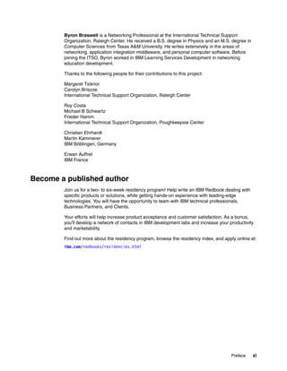
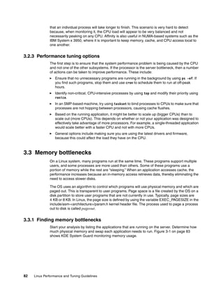
4.7.2 Speed and duplexing
One of the easiest ways to improve network performance is by checking the actual speed of
the network interface, because there can be issues between network components (such as
switches or hubs) and the network interface cards. The mismatch can have a large
performance impact as shown in Example 4-17.
Example 4-17 Using ethtool to check the actual speed and duplex settings
[root@linux ~]# ethtool eth0
Settings for eth0:
Supported ports: [ MII ]
Supported link modes: 10baseT/Half 10baseT/Full
100baseT/Half 100baseT/Full
1000baseT/Half 1000baseT/Full
Supports auto-negotiation: Yes
Advertised link modes: 10baseT/Half 10baseT/Full
100baseT/Half 100baseT/Full
1000baseT/Half 1000baseT/Full
Advertised auto-negotiation: Yes
Speed: 100Mb/s
Duplex: Full
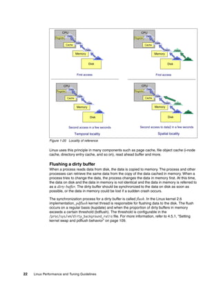
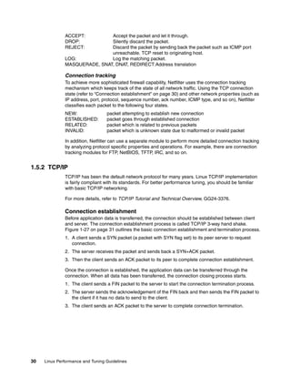
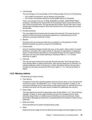
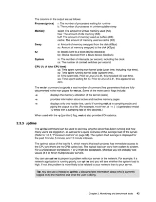
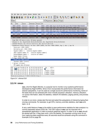
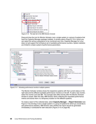
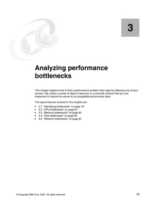
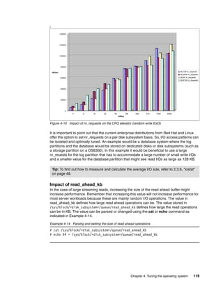
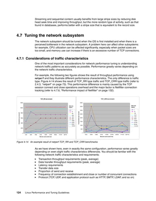
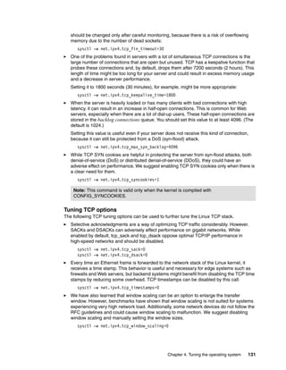
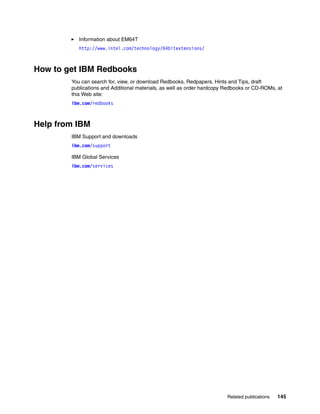
From the benchmark results shown in Figure 4-15, note that a small data transfer is less
impacted than a larger data transfer when network speeds are incorrectly negotiated. Data
transfers larger than 1 KB show drastic performance impact (throughput declines 50-90%).
Make sure that the speed and duplex are correctly set.
Figure 4-15 Performance degradation caused by auto negotiation failure
Numerous network devices default to 100 Mb half-duplex in case of a minor mismatch during
the auto negotiation process. To check for the actual line speed and duplex setting of a
network connection, use the ethtool command.
Note that most network administrators believe that the best way to attach a network interface
to the network is by specifying static speeds at both the NIC and the switch or hub port. To
100Mbsp half duplex
0.01
0.10
1.00
10.00
100.00
1,000.00
1024 2048 4096 8192 16384 32768 65536 131070 262144
socket sizes
Mbytes/sec
1
16
128
1K
4K
16K
32K
64K
128K
Response
data size
1Gbps full duplex
0.01
0.10
1.00
10.00
100.00
1,000.00
1024 2048 4096 8192 16384 32768 65536 131070 262144
socket size
Mbytes/sec
1
16
128
1K
4K
16K
32K
64K
128K
Response
data size

140. 126 Linux Performance and Tuning Guidelines
change the configuration, you can use ethtool if the device driver supports the ethtool
command. You might have to change /etc/modules.conf for some device drivers.
4.7.3 MTU size
Especially in gigabit networks, large maximum transmission units (MTU) sizes (also known as
JumboFrames) can provide better network performance. The challenge with large MTU sizes
is the fact that most networks do not support them and that a number of network cards also
do not support large MTU sizes. If your objective is transferring large amounts of data at
gigabit speeds (as in HPC environments, for example), increasing the default MTU size can
provide significant performance gains. In order to change the MTU size, use /sbin/ifconfig.
Example 4-18 Changing the MTU size with ifconfig
[root@linux ~]# ifconfig eth0 mtu 9000 up
4.7.4 Increasing network buffers
The Linux network stack is cautious when it comes to assigning memory resources to
network buffers. In modern high-speed networks that connect server systems, these values
should be increased to enable the system to handle more network packets.
򐂰 Initial overall TCP memory is calculated automatically based on system memory; you can
find the actual values in:
/proc/sys/net/ipv4/tcp_mem
򐂰 Set the default and maximum amount for the receive socket memory to a higher value:
/proc/sys/net/core/rmem_default
/proc/sys/net/core/rmem_max
򐂰 Set the default and maximum amount for the send socket to a higher value:
/proc/sys/net/core/wmem_default
/proc/sys/net/core/wmem_max
򐂰 Adjust the maximum amount of option memory buffers to a higher value:
/proc/sys/net/core/optmem_max
Tuning window sizes
Maximum window sizes can be tuned by the network buffer size parameters described above.
Theoretical optimal window sizes can be obtained by using BDP (bandwidth delay product).
BDP is the total amount of data that resides on the wire in transit. BDP is calculated with this
simple formula:
BDP = Bandwidth (bytes/sec) * Delay (or round trip time) (sec)
To keep the network pipe full and to fully utilize the line, network nodes should have buffers
available to store the same size of data as BDP. Otherwise, a sender has to stop sending data
and wait for acknowledgement to come from the receiver (refer to “Traffic control” on
page 32).
For example, in a Gigabit Ethernet LAN with 1msec delay BDP comes to:
125Mbytes/sec (1Gbit/sec) * 1msec = 125Kbytes
Attention: For large MTU sizes to work, they must be supported by both the network
interface card and the network components.

141. Chapter 4. Tuning the operating system 127
The default value of rmem_max and wmem_max is about 128 KB in most enterprise distributions,
which might be enough for a low-latency general purpose network environment. However, if
the latency is large, the default size might be too small.
Looking at another example, assuming that a samba file server has to support 16 concurrent
file transfer sessions from various locations, the socket buffer size for each session comes
down to 8 KB in default configuration. This could be relatively small if the data transfer is high.
򐂰 Set the max OS send buffer size (wmem) and receive buffer size (rmem) to 8 MB for
queues on all protocols:
sysctl -w net.core.wmem_max=8388608
sysctl -w net.core.rmem_max=8388608
These specify the amount of memory that is allocated for each TCP socket when it is
created.
򐂰 In addition, you should also use the following commands for send and receive buffers.
They specify three values: minimum size, initial size, and maximum size:
sysctl -w net.ipv4.tcp_rmem="4096 87380 8388608"
sysctl -w net.ipv4.tcp_wmem="4096 87380 8388608"
The third value must be the same as or less than the value of wmem_max and
rmem_max. However, we also suggest increasing the first value on high-speed,
high-quality networks so that the TCP windows start out at a sufficiently high value.
򐂰 Increase the values in /proc/sys/net/ipv4/tcp_mem. The three values refer to minimum,
pressure, and maximum memory allocations for TCP memory.
You can see what’s been changed by socket buffer tuning using tcpdump. As the examples
show, limiting socket buffer to small size results in small window size and causes frequent
acknowledgement packets and inefficient use (Example 4-19). On the contrary, making
socket buffer large results in a large window size (Example 4-20).
Example 4-19 Small window size (rmem, wmem=4096)
[root@lnxsu5 ~]# tcpdump -ni eth1
22:00:37.221393 IP plnxsu4.34087 > plnxsu5.32837: P 18628285:18629745(1460) ack 9088 win 46
22:00:37.221396 IP plnxsu4.34087 > plnxsu5.32837: . 18629745:18631205(1460) ack 9088 win 46
22:00:37.221499 IP plnxsu5.32837 > plnxsu4.34087: . ack 18629745 win 37
22:00:37.221507 IP plnxsu4.34087 > plnxsu5.32837: P 18631205:18632665(1460) ack 9088 win 46
22:00:37.221511 IP plnxsu4.34087 > plnxsu5.32837: . 18632665:18634125(1460) ack 9088 win 46
22:00:37.221614 IP plnxsu5.32837 > plnxsu4.34087: . ack 18632665 win 37
22:00:37.221622 IP plnxsu4.34087 > plnxsu5.32837: P 18634125:18635585(1460) ack 9088 win 46
22:00:37.221625 IP plnxsu4.34087 > plnxsu5.32837: . 18635585:18637045(1460) ack 9088 win 46
22:00:37.221730 IP plnxsu5.32837 > plnxsu4.34087: . ack 18635585 win 37
22:00:37.221738 IP plnxsu4.34087 > plnxsu5.32837: P 18637045:18638505(1460) ack 9088 win 46
22:00:37.221741 IP plnxsu4.34087 > plnxsu5.32837: . 18638505:18639965(1460) ack 9088 win 46
22:00:37.221847 IP plnxsu5.32837 > plnxsu4.34087: . ack 18638505 win 37
Example 4-20 Large window size (rmem, wmem=524288)
[root@lnxsu5 ~]# tcpdump -ni eth1
22:01:25.515545 IP plnxsu4.34088 > plnxsu5.40500: . 136675977:136677437(1460) ack 66752 win 46
22:01:25.515557 IP plnxsu4.34088 > plnxsu5.40500: . 136687657:136689117(1460) ack 66752 win 46
22:01:25.515568 IP plnxsu4.34088 > plnxsu5.40500: . 136699337:136700797(1460) ack 66752 win 46
22:01:25.515579 IP plnxsu4.34088 > plnxsu5.40500: . 136711017:136712477(1460) ack 66752 win 46
22:01:25.515592 IP plnxsu4.34088 > plnxsu5.40500: . 136722697:136724157(1460) ack 66752 win 46
22:01:25.515601 IP plnxsu4.34088 > plnxsu5.40500: . 136734377:136735837(1460) ack 66752 win 46
22:01:25.515610 IP plnxsu4.34088 > plnxsu5.40500: . 136746057:136747517(1460) ack 66752 win 46

142. 128 Linux Performance and Tuning Guidelines
22:01:25.515617 IP plnxsu4.34088 > plnxsu5.40500: . 136757737:136759197(1460) ack 66752 win 46
22:01:25.515707 IP plnxsu5.40500 > plnxsu4.34088: . ack 136678897 win 3061
22:01:25.515714 IP plnxsu5.40500 > plnxsu4.34088: . ack 136681817 win 3061
22:01:25.515764 IP plnxsu5.40500 > plnxsu4.34088: . ack 136684737 win 3061
22:01:25.515768 IP plnxsu5.40500 > plnxsu4.34088: . ack 136687657 win 3061
22:01:25.515774 IP plnxsu5.40500 > plnxsu4.34088: . ack 136690577 win 3061
Impact of socket buffer size
Small socket buffers could cause performance degradation when a server deals with a lot of
concurrent large file transfers. As Figure 4-16 shows, a clear performance decline is observed
when using small socket buffers. A low value of rmem_max and wmem_max limit available socket
buffer sizes even if the peer has affordable socket buffers available. This causes small window
sizes and creates a performance ceiling for large data transfers. Though not included in this
chart, no clear performance difference is observed for small data (less than 4 KB) transfer.
Figure 4-16 Comparison with socket buffer 4 KB and 132 bytes
4.7.5 Additional TCP/IP tuning
There are many other configuration options which can increase or decrease network
performance. The parameters we describe below can help to prevent a decrease in network
performance.
Tuning IP and ICMP behavior
The following sysctl commands are used to tune the IP and ICMP behavior:
򐂰 Disabling the following parameters prevents a cracker from using a spoofing attack against
the IP address of the server:
sysctl -w net.ipv4.conf.eth0.accept_source_route=0
sysctl -w net.ipv4.conf.lo.accept_source_route=0
tran rate per sec by recv size
0
500
1000
1500
2000
2500
3000
3500
4000
1024 2048 4096 8192 16384 32768 65536 1E+05 3E+05 5E+05
Local socket buffer size
trans
rate
per
sec
16Kbytes (rmem,wmem=132K)
32Kbytes (rmem,wmem=132K)
64Kbytes (rmem,wmem=132K)
128Kbytes (rmem,wmem=132K)
16Kbytes (wmem,rmem=4k)
32Kbytes (wmem,rmem=4k)
64Kbytes (wmem,rmem=4k)
128Kbytes (wmem,rmem=4k)
Response data size
performance
decline observed by
small socket (Local
socket buffer size is
limited to 8 KB)

143. Chapter 4. Tuning the operating system 129
sysctl -w net.ipv4.conf.default.accept_source_route=0
sysctl -w net.ipv4.conf.all.accept_source_route=0
򐂰 These commands configure the server to ignore redirects from machines that are listed as
gateways. Redirect can be used to perform attacks, so we only want to allow them from
trusted sources:
sysctl -w net.ipv4.conf.eth0.secure_redirects=1
sysctl -w net.ipv4.conf.lo.secure_redirects=1
sysctl -w net.ipv4.conf.default.secure_redirects=1
sysctl -w net.ipv4.conf.all.secure_redirects=1
򐂰 You could allow the interface to accept or not accept any ICMP redirects. The ICMP
redirect is a mechanism for routers to convey routing information to hosts. For example,
the gateway can send a redirect message to a host when the gateway receives an Internet
datagram from a host on a network to which the gateway is attached. The gateway checks
the routing table to get the address of the next gateway, and the second gateway routes
the Internet datagram to the network destination. Disable these redirects using the
following commands:
sysctl -w net.ipv4.conf.eth0.accept_redirects=0
sysctl -w net.ipv4.conf.lo.accept_redirects=0
sysctl -w net.ipv4.conf.default.accept_redirects=0
sysctl -w net.ipv4.conf.all.accept_redirects=0
򐂰 If this server does not act as a router, it does not have to send redirects, so they can be
disabled:
sysctl -w net.ipv4.conf.eth0.send_redirects=0
sysctl -w net.ipv4.conf.lo.send_redirects=0
sysctl -w net.ipv4.conf.default.send_redirects=0
sysctl -w net.ipv4.conf.all.send_redirects=0
򐂰 Configure the server to ignore broadcast pings and smurf attacks:
sysctl -w net.ipv4.icmp_echo_ignore_broadcasts=1
򐂰 Ignore all kinds of icmp packets or pings:
sysctl -w net.ipv4.icmp_echo_ignore_all=1
򐂰 Some routers send invalid responses to broadcast frames, and each one generates a
warning that is logged by the kernel. These responses can be ignored:
sysctl -w net.ipv4.icmp_ignore_bogus_error_responses=1
򐂰 We should set the ipfrag parameters, particularly for NFS and Samba servers. Here, we
can set the maximum and minimum memory used to reassemble IP fragments. When the
value of ipfrag_high_thresh in bytes of memory is allocated for this purpose, the fragment
handler will drop packets until ipfrag_low_thresh is reached.
Fragmentation occurs when there is an error during the transmission of TCP packets.
Valid packets are stored in memory (as defined with these parameters) while corrupted
packets are retransmitted.
For example, to set the range of available memory to between 256 MB and 384 MB, use:
sysctl -w net.ipv4.ipfrag_low_thresh=262144
sysctl -w net.ipv4.ipfrag_high_thresh=393216

144. 130 Linux Performance and Tuning Guidelines
Tuning TCP behavior
Here we describe tuning parameters that will change TCP behaviors.
The following commands can be used for tuning servers that support a large number of
multiple connections:
򐂰 For servers that receive many connections at the same time, the TIME-WAIT sockets for
new connections can be reused. This is useful in Web servers, for example:
sysctl -w net.ipv4.tcp_tw_reuse=1
If you enable this command, you should also enable fast recycling of TIME-WAIT sockets
status:
sysctl -w net.ipv4.tcp_tw_recycle=1
Figure 4-17 shows that with these parameters enabled, the number of connections is
significantly reduced. This is good for performance because each TCP transaction
maintains a cache of protocol information about each of the remote clients. In this cache,
information such as round-trip time, maximum segment size, and congestion window are
stored. For more details, review RFC 1644.
Figure 4-17 Parameters reuse and recycle enabled (left) and disabled (right)
򐂰 The parameter tcp_fin_timeout is the time to hold a socket in state FIN-WAIT-2 when the
socket is closed at the server.
A TCP connection begins with a three-segment synchronization SYN sequence and ends
with a three-segment FIN sequence, neither of which holds data. By changing the
tcp_fin_timeout value, the time from the FIN sequence to when the memory can be freed
for new connections can be reduced, thereby improving performance. This value, however,
With both
tcp_tw_reuse and
tcp_tw_recycle
enabled, the
information about
the hosts does not
have to be obtained
again and the TCP
transaction can
start immediately,
preventing the
unnecessary traffic.
tcp_tw_reuse and
tcp_tw_recycle
enabled.
tcp_tw_reuse and
tcp_tw_recycle
disabled.

145. Chapter 4. Tuning the operating system 131
should be changed only after careful monitoring, because there is a risk of overflowing
memory due to the number of dead sockets:
sysctl -w net.ipv4.tcp_fin_timeout=30
򐂰 One of the problems found in servers with a lot of simultaneous TCP connections is the
large number of connections that are open but unused. TCP has a keepalive function that
probes these connections and, by default, drops them after 7200 seconds (2 hours). This
length of time might be too long for your server and could result in excess memory usage
and a decrease in server performance.
Setting it to 1800 seconds (30 minutes), for example, might be more appropriate:
sysctl -w net.ipv4.tcp_keepalive_time=1800
򐂰 When the server is heavily loaded or has many clients with bad connections with high
latency, it can result in an increase in half-open connections. This is common for Web
servers, especially when there are a lot of dial-up users. These half-open connections are
stored in the backlog connections queue. You should set this value to at least 4096. (The
default is 1024.)
Setting this value is useful even if your server does not receive this kind of connection,
because it can still be protected from a DoS (syn-flood) attack.
sysctl -w net.ipv4.tcp_max_syn_backlog=4096
򐂰 While TCP SYN cookies are helpful in protecting the server from syn-flood attacks, both
denial-of-service (DoS) or distributed denial-of-service (DDoS), they could have an
adverse effect on performance. We suggest enabling TCP SYN cookies only when there is
a clear need for them.
sysctl -w net.ipv4.tcp_syncookies=1
Tuning TCP options
The following TCP tuning options can be used to further tune the Linux TCP stack.
򐂰 Selective acknowledgments are a way of optimizing TCP traffic considerably. However.
SACKs and DSACKs can adversely affect performance on gigabit networks. While
enabled by default, tcp_sack and tcp_dsack oppose optimal TCP/IP performance in
high-speed networks and should be disabled.
sysctl -w net.ipv4.tcp_sack=0
sysctl -w net.ipv4.tcp_dsack=0
򐂰 Every time an Ethernet frame is forwarded to the network stack of the Linux kernel, it
receives a time stamp. This behavior is useful and necessary for edge systems such as
firewalls and Web servers, but backend systems might benefit from disabling the TCP time
stamps by reducing some overhead. TCP timestamps can be disabled by this call:
sysctl -w net.ipv4.tcp_timestamps=0
򐂰 We have also learned that window scaling can be an option to enlarge the transfer
window. However, benchmarks have shown that window scaling is not suited for systems
experiencing very high network load. Additionally, some network devices do not follow the
RFC guidelines and could cause window scaling to malfunction. We suggest disabling
window scaling and manually setting the window sizes.
sysctl -w net.ipv4.tcp_window_scaling=0
Note: This command is valid only when the kernel is compiled with
CONFIG_SYNCOOKIES.

146. 132 Linux Performance and Tuning Guidelines
4.7.6 Performance impact of Netfilter
As Netfilter provides TCP/IP connection tracking and packet filtering capability (refer to
“Netfilter” on page 29), in certain circumstances it may have a large performance impact. The
impact is clearly visible when the number of connection establishments is high. Figure 4-18
and Figure 4-19 show benchmark results with large and small connection establishments
counts. The results clearly illustrate the effect of the Netfilter.
When no Netfilter rule is applied (Figure 4-18), the result shows similar performance
characteristics to a benchmark where connection establishment rarely occurs (refer to the left
chart of Figure 4-14 on page 124) while absolute throughput still differs because of
connection establishment overhead.
Figure 4-18 No Netfilter rule applied
However, when filtering rules are applied, relatively inconsistent behavior can been seen
(Figure 4-19).
Figure 4-19 Netfilter rules applied
TCP_CRRbenchmark
0
500
1000
1500
2000
2500
3000
3500
4000
4500
1024 2048 4096 8192 16384 32768 65536 131070 262144
remote sendsocket size
trans
rate
per
sec
1
16
128
1024
1460
4096
16384
32768
65536
131072
Data size
(bytes)
TCP_CRRbenckmark
0
500
1000
1500
2000
2500
3000
3500
4000
4500
1 16 128 1024 1460 4096 16384 32768 65536 131072
receivedatasize
tran
rate
1024
2048
4096
8192
16384
32768
65536
131070
262144
524288
Socket size
(bytes)
TCP_CRRbenchmark
0
500
1000
1500
2000
2500
3000
3500
4000
1024 2048 4096 8192 16384 32768 65536 131070 262144
Remote sendsocket size
Transactions
per
second
1
16
128
1024
1460
4096
16384
32768
65536
131072
Data size
(bytes)
TCP_CRRbanchmark
0
500
1000
1500
2000
2500
3000
3500
4000
1 16 128 1024 1460 4096 16384 32768 65536 131072
receivedatasize
trans
per
sec
1024
2048
4096
8192
16384
32768
65536
131070
262144
524288
Socket size
(bytes)

147. Chapter 4. Tuning the operating system 133
However, Netfilter provides packet filtering capability and enhances network security. It can be
a trade-off between security and performance. The Netfilter performance impact depends on
the following factors:
򐂰 Number of rules
򐂰 Order of rules
򐂰 Complexity of rules
򐂰 Connection tracking level (depends on protocols)
򐂰 Netfilter kernel parameter configuration
4.7.7 Offload configuration
As we described in 1.5.3, “Offload” on page 33, some network operations can be offloaded to
a network interface device if it supports the capability. You can use the ethtool command to
check the current offload configurations.
Example 4-21 Checking offload configurations
[root@lnxsu5 plnxsu4]# ethtool -k eth0
Offload parameters for eth0:
rx-checksumming: off
tx-checksumming: off
scatter-gather: off
tcp segmentation offload: off
udp fragmentation offload: off
generic segmentation offload: off
Change the configuration command syntax is as follows:
ethtool -K DEVNAME [ rx on|off ] [ tx on|off ] [ sg on|off ] [ tso on|off ] [
ufo on|off ] [ gso on|off ]
Example 4-22 Example of offload configuration change
[root@lnxsu5 plnxsu4]# ethtool -k eth0 sg on tso on gso off
Supported offload capability might differ by network interface device, Linux distribution, kernel
version, and the platform you choose. If you issue an unsupported offload parameter, you
might get error messages.
Impact of offloading
Benchmarks have shown that the CPU utilization can be reduced by NIC offloading.
Figure 4-20 on page 134 shows the higher CPU utilization improvement in large data size
(more than 32 KB). The large packets take advantage of checksum offloading because
checksumming needs to calculate the entire packet, so more processing power is consumed
as the data size increases.

148. 134 Linux Performance and Tuning Guidelines
Figure 4-20 CPU usage improvement by offloading
However, a slight performance degradation is observed in using offloading (Figure 4-21). The
processing of checksums for such a high packet rate is a significant load on certain LAN
adapter processors. As the packet size gets larger, fewer packets per second are being
generated (because it takes a longer time to send and receive all that data) and it is prudent
to offload the checksum operation on to the adapter.
Figure 4-21 Throughput degradation by offloading
CPU usage improvement - default vs offload off
0
1
2
3
4
5
6
7
8
1 16 128 1024 1460 4096 16384 32768 65536 131072
recv data size
CPU
usage
improvement
(%)
2048
4096
8192
16384
32768
65536
131070
262144
socket size
(bytes)
Throughput degradation ratio
default vs offload by socket size
0.82
0.84
0.86
0.88
0.9
0.92
0.94
0.96
0.98
1
1.02
1 16 128 1024 1460 4096 16384 32768 65536 1E+05
recv data size
tps
offload
/
tps
def
1024
2048
4096
8192
16384
32768
65536
131070
262144
socket size
(bytes)

149. Chapter 4. Tuning the operating system 135
LAN adapters are efficient when network applications requesting data generate requests for
large frames. Applications that request small blocks of data require the LAN adapter
communication processor to spend a greater percentage of time executing overhead code for
every byte of data transmitted. This is why most LAN adapters cannot sustain full wire speed
for all frame sizes.
Refer to Tuning IBM System x Servers for Performance, SG24-5287. section 10.3. Advanced
network features for more details.
4.7.8 Increasing the packet queues
After increasing the size of the various network buffers, it is recommended that the amount of
allowed unprocessed packets be increased, so that the kernel will wait longer before dropping
packets. To do so, edit the value in /proc/sys/net/core/netdev_max_backlog.
4.7.9 Increasing the transmit queue length
Increase the txqueuelength parameter to a value between 1000 and 20000 per interface. This
is especially useful for high-speed connections that perform large, homogeneous data
transfers. The transmit queue length can be adjusted by using the ifconfig command as
shown in Example 4-23.
Example 4-23 Setting the transmit queue length
[root@linux ipv4]# ifconfig eth1 txqueuelen 2000
4.7.10 Decreasing interrupts
Handling network packets requires the Linux kernel to handle a significant amount of
interrupts and context switches unless NAPI is being used. For Intel e1000–based network
interface cards, make sure that the network card driver was compiled with the
CFLAGS_EXTRA -DCONFIG_E1000_NAPI flag. Broadcom tg3 modules should come in
their newest version with built in NAPI support.
If you need to recompile the Intel e1000 driver in order to enable NAPI, you can do so by
issuing the following command on your build system:
make CFLAGS_EXTRA -DCONFIG_E1000_NAPI
In addition, on multiprocessor systems, binding the interrupts of the network interface cards to
a physical CPU might yield additional performance gains. To achieve this goal you first have
to identify the IRQ by the respective network interface. The data obtained via the ifconfig
command will inform you of the interrupt number.
Example 4-24 Identifying the interrupt
[root@linux ~]# ifconfig eth1
eth1 Link encap:Ethernet HWaddr 00:11:25:3F:19:B3
inet addr:10.1.1.11 Bcast:10.255.255.255 Mask:255.255.0.0
inet6 addr: fe80::211:25ff:fe3f:19b3/64 Scope:Link
UP BROADCAST RUNNING MULTICAST MTU:1500 Metric:1
RX packets:51704214 errors:0 dropped:0 overruns:0 frame:0
TX packets:108485306 errors:0 dropped:0 overruns:0 carrier:0
collisions:0 txqueuelen:1000
RX bytes:4260691222 (3.9 GiB) TX bytes:157220928436 (146.4 GiB)
Interrupt:169

150. 136 Linux Performance and Tuning Guidelines
After obtaining the interrupt number, you can use the smp_affinity parameter found in
/proc/irq/%{irq number} to tie an interrupt to a CPU. Example 4-25 illustrates this for the
above output of interrupt 169 of eth1 being bound to the second processor in the system.
Example 4-25 Setting the CPU affinity of an interrupt
[root@linux ~]# echo 02 > /proc/irq/169/smp_affinity

151. © Copyright IBM Corp. 2007. All rights reserved. 137
Appendix A. Testing configurations
This appendix lists the hardware and software configurations used to load and test various
tuning parameters, monitoring software, and benchmark runs.
A

152. 138 Linux Performance and Tuning Guidelines
Hardware and software configurations
The tests, tuning modifications, benchmark runs, and monitoring performed for this redpaper
were executed with Linux installed on two different hardware platforms:
򐂰 Guest on IBM z/VM systems
򐂰 Native on IBM System x servers
Linux installed on guest IBM z/VM systems
IBM z/VM V5.2.0 was installed on an LPAR on an IBM z9 processor. Installed z/VM
components were tcpip, dirmaint, rscs, pvm, and vswitch.
The various Linux guest VM systems were configured as shown in Table A-1.
Table A-1 Linux installed on guest z/VM systems
Linux installed on IBM System x servers
Three IBM System x x236 servers were configured as shown in Table A-2.
Table A-2 Linux installed on System x servers
System name LNXSU1 LNXSU2 LNXRH1
Linux distribution SUSE Linux
Enterprise Server 10
SUSE Linux
Enterprise Server 10
Red Hat Enterprise
Linux 5
Install default with sysstat
6.0.2-16.4
default with sysstat
6.0.2-16.4
default with sysstat
7.0.0-3.el5
Memory 512 MB 512 MB 512 MB
swap (2105 Shark
DASD)
710 MB 710 MB 710 MB
/root (2105 Shark
DASD)
6.1 GB 6.1 GB 6.1 GB
/perf (2107 DS8000
DASD)
ReiserFS 6.8 GB Ext3 6.8 GB Ext3 6.8 GB
System name LNXSU3 LNXSU4 LNXSU5
Linux distribution SUSE Linux
Enterprise Server 10
(runlevel 3)
Red Hat Enterprise
Linux 4
(runlevel 5)
Red Hat Enterprise
Linux 5
(runlevel 5)
Install default with sysstat
6.0.2-16.4 and
powertweak
default with sysstat default with sysstat
Memory 4096 MB 4096 MB 4096 MB
swap (RAID 1,
2*74GB)
2 GB 2 GB 2 GB
/root (RAID 1, 2*74GB) 70 GB 70 GB 70 GB

153. Appendix A. Testing configurations 139
/perf (RAID 5EE,
4*74GB)
ReiserFS 200 GB Ext3 200 GB Ext3 200 GB

154. 140 Linux Performance and Tuning Guidelines

155. © Copyright IBM Corp. 2007. All rights reserved. 141
ACK acknowledgment character
ACPI Advanced Configuration and Power Interface
AIX Advanced Interactive eXecutive
API application programming interface
ATA AT Attachment
AVC Access Vector Cache
BDP bandwidth delay product
BSD Berkeley Software Distribution
BSS block storage segment
CEC central electronics complex
CFQ Complete Fair Queuing
CPU central processing unit
CSV comma separated values
CUPS Common UNIX Printing System
DF decision federator
DMA direct memory access
DNAT dynamic network address translation
DNS Domain Name System
DS directory services
FAT file allocation table
FIFO first-in-first-out
FQDN fully qualified domain name
FS fibre-channel service
FTP File Transfer Protocol
GNU GNU’s Not Unix
GPL general public license
GRUB grand unified bootloader
GUI Graphical User Interface
HBA host bus adapter
HPC high performance computing
HTML Hypertext Markup Language
HTTP Hypertext Transfer Protocol
IBM International Business Machines Corporation
ICMP Internet Control Message Protocol
IDE integrated drive electronics
IP Internet Protocol
IRC interregion communication
IRQ interrupt request
ISV independent software vendor
ITSO International Technical Support Organization
Abbreviations and acronyms
JFS Journal File System
KDE K Desktop Environment
LAN local area network
LDAP Lightweight Directory Access Protocol
LIFO last-in first-out
LRU Least Recently Used
LSI large-scale integration
LSM Linux Security Modules
LWP Light Weight Process
MAC Medium Access Control
MTU maximum transmission units
NAPI network API
NFS Network File System
NGPT Next Generation POSIX Thread
NIC Network Information Center
NLWP number of light weight processes
NOOP no operation
NPTL Native POSIX Thread Library
NUMA Non-Uniform Memory Access
OSI open systems interconnection
PC path control
PCI Peripheral Component Interconnect
PID process ID
POSIX Portable Operating System Interface for
Computer Environments
PPID parent process ID
PRI primary rate interface
RAID Redundant Array of Independent Disks
RAM random access memory
RFC Request for Comments
RPM Redhat Package Manager
RSS rich site summary
SACK selective acknowledgment
SATA Serial ATA
SCSI Small Computer System Interface
SMP symmetric multiprocessor
SMT symmetric multithreading
SMTP Simple Mail Transport Protocol
SUSE Software Und System Entwicklung
SWAT Samba Web Administration Tool

156. 142 Linux Performance and Tuning Guidelines
SYN synchronization character
TCQ Tagged Command Queuing
TFTP Trivial File Transfer Protocol
TLB Translation Lookaside Buffer
TSO TCP segmentation offload
TTY teletypewriter
UDP User Datagram Protocol
UID unique identifier
UP uniprocessor
USB Universal Serial Bus
VFS Virtual Files System
VM virtual machine
XFS eXtended File System
XML Extensible Markup Language
YaST yet another setup tool

157. © Copyright IBM Corp. 2007. All rights reserved. 143
Related publications
The publications listed in this section are considered particularly suitable for a more detailed
discussion of the topics covered in this paper.
IBM Redbooks
For information about ordering these publications, see “How to get IBM Redbooks” on
page 145. Note that some of the documents referenced here may be available in softcopy
only.
򐂰 Linux Handbook A Guide to IBM Linux Solutions and Resources, SG24-7000
򐂰 Tuning IBM System x Servers for Performance, SG24-5287
򐂰 IBM System Storage Solutions Handbook, SG24-5250
򐂰 IBM TotalStorage Productivity Center for Replication on Linux, SG24-7411
򐂰 Introduction to Storage Area Networks, SG24-5470
򐂰 TCP/IP Tutorial and Technical Overview, GG24-3376
Other publications
These publications are also relevant as further information sources:
򐂰 Beck, M., et al., Linux Kernel Internals, Second Edition, Addison-Wesley Pub Co, 1997,
ISBN 0201331438
򐂰 Bovet, Daniel P., Cesati, Marco, Understanding the Linux Kernel, O’Reilly Media, Inc.
2005, ISBN-10: 0596005652
򐂰 Kabir, M., Red Hat Linux Security and Optimization. John Wiley & Sons, 2001,
ISBN 0764547542
򐂰 Musumeci, Gian-Paolo D., Loukides, Mike, System Performance Tuning, 2nd Edition,
O’Reilly Media, Inc. 2002, ISBN-10: 059600284X
򐂰 Stanfield, V., et al., Linux System Administration, Second Edition, Sybex Books, 2002,
ISBN 0782141382
Online resources
These Web sites are also relevant as further information sources:
򐂰 Linux Networking Scalability on High-Performance Scalable Servers
http://www.ibm.com/servers/eserver/xseries/benchmarks/
򐂰 Linux tuning hints and tips on System z
http://www.ibm.com/developerworks/linux/linux390/perf/index.html
򐂰 System Tuning Info for Linux Servers
http://people.redhat.com/alikins/system_tuning.html
򐂰 Securing and Optimizing Linux (Red Hat 6.2)

158. 144 Linux Performance and Tuning Guidelines
http://www.faqs.org/docs/securing/index.html
򐂰 Linux 2.6 Performance in the Corporate Data Center
http://www.osdl.org/docs/linux_2_6_datacenter_performance.pdf
򐂰 Developer of ReiserFS
http://www.namesys.com
򐂰 New features of V2.6 kernel
http://www.infoworld.com/infoworld/article/04/01/30/05FElinux_1.html
򐂰 WebServing on 2.4 and 2.6
http://www.ibm.com/developerworks/linux/library/l-web26/
򐂰 man page about the ab command
http://cmpp.linuxforum.net/cman-html/man1/ab.1.html
򐂰 Network Performance improvements in Linux 2.6
http://developer.osdl.org/shemminger/LWE2005_TCP.pdf
򐂰 RADIANT Publications and Presentations
http://public.lanl.gov/radiant/pubs.html
򐂰 RFC: Multicast
http://www.ietf.org/rfc/rfc2365.txt
򐂰 RFC: Internet Control Message Protocol
http://www.networksorcery.com/enp/RFC/Rfc792.txt
򐂰 RFC: Fault Isolation and Recovery
http://www.networksorcery.com/enp/RFC/Rfc816.txt
򐂰 RFC: Type of Service in the Internet Protocol Suite
http://www.networksorcery.com/enp/rfc/rfc1349.txt
򐂰 Performance Tuning with OpenLDAP
http://www.openldap.org/faq/data/cache/190.html
򐂰 RFC: TCP Extensions for Long-Delay Paths
http://www.cse.ohio-state.edu/cgi-bin/rfc/rfc1072.html
򐂰 RFC: TCP Extensions for High Performance
http://www.cse.ohio-state.edu/cgi-bin/rfc/rfc1323.html
򐂰 RFC: Extending TCP for Transactions -- Concepts
http://www.cse.ohio-state.edu/cgi-bin/rfc/rfc1379.html
򐂰 RFC: T/TCP -- TCP Extensions for Transactions
http://www.cse.ohio-state.edu/cgi-bin/rfc/rfc1644.html
򐂰 LOAD - Load and Performance Test Tools
http://www.softwareqatest.com/qatweb1.html
򐂰 The Web100 Project
http://www.web100.org/
򐂰 Information about Hyper-Threading
http://www.intel.com/business/bss/products/hyperthreading/server/

159. Related publications 145
򐂰 Information about EM64T
http://www.intel.com/technology/64bitextensions/
How to get IBM Redbooks
You can search for, view, or download Redbooks, Redpapers, Hints and Tips, draft
publications and Additional materials, as well as order hardcopy Redbooks or CD-ROMs, at
this Web site:
ibm.com/redbooks
Help from IBM
IBM Support and downloads
ibm.com/support
IBM Global Services
ibm.com/services

160. 146 Linux Performance and Tuning Guidelines

161. © Copyright IBM Corp. 2007. All rights reserved. 147
Index
Symbols
/proc
parameter files in 107
Numerics
32-bit architectures 10
3-way hand shake 30
64-bit architectures 11
A
Access Vector Cache 104
ACK packet 30
ACPI
See advanced configuration and power interface
advanced configuration and power interface 61
anticipatory 24, 116–117
apmd 97
arptables 97
autofs 97
AVC
See Access Vector Cache
B
bandwidth delay product 126
benchmark tools 70–76
functions overview 40
IOzone 72
LMbench 71
netperf 73–75
bind a process to a CPU 81
bind an interrupt to a CPU 6, 108
block device metrics 36
block layer 23–24
block size 123
bonding driver 34
bonding module 34
bottlenecks
analyzing the server’s performance 80
CPU bottlenecks 81–82
disk bottlenecks 84–87
gathering information 78
memory bottlenecks 82–84
network bottlenecks 87–89
bus subdirectory 62
C
C09 compiler flag 104
cache 21–22
cache optimization 81
Capacity Manager 67–70
cat command 105, 107
CFQ
See Complete Fair Queuing
change management 92
changing kernel parameters 104–107
checksum offload 33
child process 3
chkconfig command 98
clone() 5
collision packets 88
compiling the kernel 104
Complete Fair Queuing 24, 115–118, 121
connection establishment 30
3-way hand shake 30
connection tracking 30
context 5
context switching 5
CPU affinity 81
CPU bottlenecks 81–82
actions 82
CPU scheduler 9–10
cpuinfo command 61
cpuspeed 97
cups 97
D
daemons 97–100
default 97
tunable 97
data segment 8
deadline 24, 115–117
dirty buffer 22, 109
flushing 22, 110
dirty_ratio 110
disable SELinux 103
disc drives 113
disk bottlenecks 84–87
iostat command 86
solutions 87
vmstat command 85
disk I/O subsystem 19–25
block layer 23–24
cache 21–22
I/O subsystem architecture 20
disk subsystem 112–124
adding drives 87
file system selection 120–124
file system tuning 120–124
hardware considerations 113
I/O elevator selection 115–119
I/O elevator tuning 115–119
dmesg command 94
dropped packets 88
duplexing 125
dynamic memory allocation 8

162. 148 Linux Performance and Tuning Guidelines
E
elevator
See I/O elevator
Enterprise Linux distributions 93
ethereal command 55, 57
ethtool command 125–126
exec() 4
exit() 4
Ext2 17–18, 120
Ext3 18–19, 120, 122
extended 2 file system
See Ext2
extended 3 file system
See Ext3
eXtended File System 19, 120
F
faulty adapters 88
Fibre Channel controllers 85
file system 15–19
Ext2 17–18
Ext3 18–19
eXtended File System 19
Journal File System 19
journaling 16
ReiserFS 19
selection 120–124
tuning 120–124
virtual file system 15
file system selection 93
FIN packet 30
fork() 3
free command 46
memory used in a zone 47
G
getty 15
Gnome System Monitor 67
gpm 97
H
hardware considerations 113
hpoj 97
HugeTLBfs 111
I
I/O elevator 20, 23–24, 113, 115–119
anticipatory 24, 116–117
Complete Fair Queuing 24, 115–118, 121
deadline 24, 115–117
NOOP 24, 116–117
selection 115–119
tuning 115–119
I/O subsystem architecture 20
IBM Director 67
init command 101
installation considerations 92–104
interrupt handling 6
bind an interrupt to a CPU 6, 108
CPU affinity 108
interrupts
decreasing 135
ionice 121
iostat command 48, 86
IOzone 72
iptraf 54
irq subdirectory 62
irqbalance 97
isdn 97
J
JFS
See Journal File System
Journal File System 19, 120, 122
journaling 16, 112
mode 122
K
KDE System Guard 62–67, 82
Process Table 65
System Load 64
kernel
changing parameters 104–107
compiling 104
swap behavior 109
view current configuration 105
kernel panic 87
kudzu 97
L
LD_ASSUME_KERNEL 5
libpcap library 55
Light Weight Process 4
Linux
distributions 93
installation considerations 92–104
performance metrics 34–37
Linux Security Modules 104
LinuxThreads 4
LMbench 71
locality of reference 21
LSM
See Linux Security Modules
LWP
See Light Weight Process
M
maximum transmission unit 33, 126–128
size 126
memory
32-bit architectures 10
64-bit architectures 11
memory architecture 10–15
memory bottlenecks 82–84
actions 84

163. Index 149
memory hierarchy 21
memory metrics 35
memory used in a zone 47
mmap() 111
monitoring tools 41–70
Capacity Manager 67–70
ethereal command 55, 57
free command 46
functions overview 40
Gnome System Monitor 67
iostat command 48
iptraf 54
KDE System Guard 62–67
mpstat command 51
netstat 53
nmon 58
numastat command 52
pmap command 52
proc file system 60–62
ps command 44
pstree command 44
sar command 50
strace command 59
tcpdump command 55–56
top command 41
uptime command 43
vmstat command 42
mount command 122
mpstat command 51
MTU
See maximum transmission unit
N
NAPI
See network API
Native POSIX Thread Library 5
net subdirectory 62
Netfilter 29–30
connection tracking 30
performance impact 132–133
usage considerations 94
netfs 98
netperf 73–75, 124
netstat 53
network API 28–29
network bottlenecks 87–89
network buffers 126
socket buffer size 128
tuning window sizes 126
network interface metrics 36
network subsystem 26–34, 124–136
duplexing 125
maximum transmission unit 126–128
Netfilter
performance impact 132–133
network buffers 126
offload
configuration 133–135
TCP/IP 30–34
TCP/IP tuning 128–131
traffic characteristics 124
networking implementation
Netfilter 29–30
network API 28–29
network subsystem
networking implementation 26–30
Next Generation POSIX Thread 5
nfslock 98
NGPT
See Next Generation POSIX Thread
nice command 108
nice level 5, 108
Nigel's Monitor 58
nmon 58
noatime 122
Non-Uniform Memory Architecture 9, 52, 108
NOOP 24, 116–117
NPTL
See Native POSIX Thread Library
nr_requests 117
NUMA
See Non-Uniform Memory Architecture
numastat command 52, 109
number of disk drives 113
O
O(1) algorithm 9
O(n) algorithm 9
offload 33
checksum offload 33
configuration 133–135
impact 133
TCP segmentation offload 33
P
package selection considerations 94
packet queues 135
page cache 20
paging
compared to swapping 83
defined 83
partition layout considerations 93
partitions
setting up 114–115
pcmcia 98
pdflush 20, 22, 109
pdflush behavior 109
pmap command 8, 52
Portable Operating System Interface for UNIX 4
portmap 98
POSIX
See Portable Operating System Interface for UNIX
powertweak 106
proc file system 60–62
ACPI 61
bus subdirectory 62
changing kernel settings 104
irq subdirectory 62
net subdirectory 62

164. 150 Linux Performance and Tuning Guidelines
scsi subdirectory 62
sys subdirectory 62
tty subdirectory 62
process
child 3
defined 2
descriptor 3
lifecycle 3
process management 2–10
process memory segments
data segment 8
stack segment 8
text segment 8
process priority 5
arrays 9
tuning 108
process state
TASK_INTERRUPTIBLE 6
TASK_RUNNING 6
TASK_STOPPED 6
TASK_UNINTERRUPTIBLE 7
TASK_ZOMBIE 7
Process Table 65
processor metrics 34
processor subsystem, tuning 107–109
ps command 44
pstree command 44
pthread 4
Q
Quality of Service
Complete Fair Queuing 24
R
RAID 87, 113, 123
RAID-0 85
RAID-10 85
RAID-5 85
rawdevices 98
read_ahead_kb 119
Redbooks Web site 145
Contact us xii
redundant array of independent disks
See RAID
ReiserFS 19, 120, 122
renice command 108
retransmission 33
rpc 98
runlevel
changing 101
selection 94
runlevel command 101
S
sa1 50
sa2 50
sar command 50
SCSI
See Small Computer System Interface
SCSI buses 85
scsi subdirectory 62
Security Enhanced Linux
See SELinux
SELinux 94, 102–104
disabling 103
sendmail 98
sequential workloads 85
Small Computer System Interface 24
smartd 98
SMP 81
SMT
See symmetric multithreading
socket buffer 26–27
socket buffer size 128
socket interface 26
speed 125
stack segment 8
strace command 59
streaming 85
stripe size 123
stripe-unit size 123
swap file 12, 93
compared to swap partition 93
swap partition 15, 93, 110–111
compared to swap file 93
multiple 110
swap space 13
swapping
compared to paging 83
defined 83
symmetric multithreading 108
SYN packet 30
sys subdirectory 62
sysctl command 105, 107, 128
system call
clone() 5
exec() 4
exit() 4
fork() 3
wait() 4
System Load 64
T
TASK_INTERRUPTIBLE 6
TASK_RUNNING 6
TASK_STOPPED 6
TASK_UNINTERRUPTIBLE 7
TASK_ZOMBIE 7
TCP segmentation offload 33
TCP/IP 30–34
bonding module 34
connection establishment 30
offload 33
retransmission 33
traffic control 32
transfer window 32
tuning 128–131
tcpdump 127

165. Index 151
tcpdump command 55–56
text segment 8
thread 4–5
defined 4
LD_ASSUME_KERNEL 5
Light Weight Process 4
LinuxThreads 4
Native POSIX Thread Library 5
Next Generation POSIX Thread 5
top command 41
traffic characteristics 124
traffic control 32
transfer window 32
Translation Lookaside Buffer 111
transmit queue length 135
TSO
See TCP segmentation offload
tty subdirectory 62
tunable daemons 97
tuning
disk subsystem 112–124
ICMP 128
IP 128
network subsystem 124–136
processor subsystem 107–109
TCP 130
TCP options 131
virtual memory subsystem 109–112
window sizes 126
U
ulimit command 96
uptime command 43, 81
V
VFS
See virtual file system
virtual file system 15
virtual memory 10
virtual memory manager 12
virtual memory subsystem 109–112
virtual terminals 102
vmstat command 42, 51, 61, 85
W
wait() 4
X
XFS
See eXtended File System
xfs 98
Z
zombie processes 7

166. 152 Linux Performance and Tuning Guidelines

168. ®
REDP-4285-00
INTERNATIONAL
TECHNICAL
SUPPORT
ORGANIZATION
BUILDING TECHNICAL
INFORMATION BASED ON
PRACTICAL EXPERIENCE
IBM Redbooks are developed
by the IBM International
Technical Support
Organization. Experts from
IBM, Customers and Partners
from around the world create
timely technical information
based on realistic scenarios.
Specific recommendations
are provided to help you
implement IT solutions more
effectively in your
environment.
For more information:
ibm.com/redbooks
Redpaper
Linux Performance and
Tuning Guidelines
Operating system
tuning methods
Performance
monitoring tools
Performance analysis
IBM® has embraced Linux, and it is recognized as an operating
system suitable for enterprise-level applications running on IBM
systems. Most enterprise applications are now available on Linux,
including file and print servers, database servers, Web servers, and
collaboration and mail servers.
With use of Linux in an enterprise-class server comes the need to
monitor performance and, when necessary, tune the server to remove
bottlenecks that affect users. This IBM Redpaper describes the
methods you can use to tune Linux, tools that you can use to monitor
and analyze server performance, and key tuning parameters for
specific server applications. The purpose of this redpaper is to
understand, analyze, and tune the Linux operating system to yield
superior performance for any type of application you plan to run on
these systems.
The tuning parameters, benchmark results, and monitoring tools used
in our test environment were executed on Red Hat and Novell SUSE
Linux kernel 2.6 systems running on IBM System x servers and IBM
System z servers. However, the information in this redpaper should be
helpful for all Linux hardware platforms.
Back cover