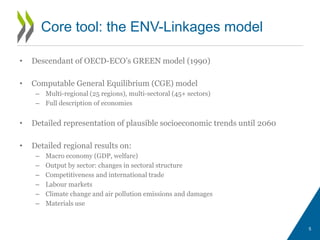
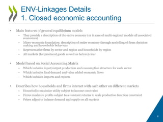
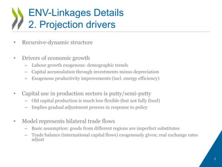
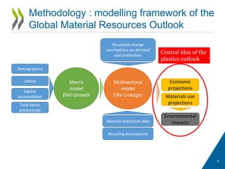
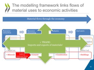
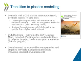
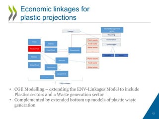
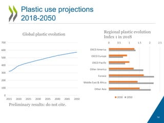
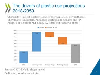
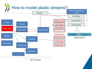
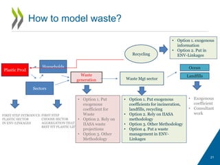
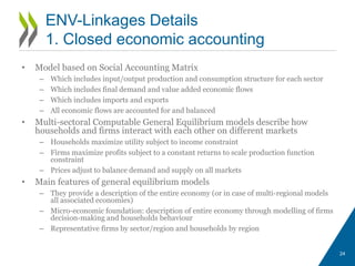
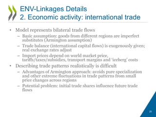
Global plastic projections are expected to rise substantially through 2050 without new policy interventions. A structural economic model called ENV-Linkages can provide insights into the underlying economic drivers of plastic use projections on a sectoral level. ENV-Linkages is a multi-regional, multi-sectoral computable general equilibrium model that can track the entire plastic value chain. It allows for sector-based plastic projections and considers issues like international trade, costs and benefits of policies, and coordinated policy action across different areas. There are ongoing efforts to extend ENV-Linkages to explicitly include plastic sectors and waste generation.

1. GLOBAL PLASTIC PROJECTIONS TO
2050: ECONOMIC DRIVERS AND
ENVIRONMENTAL CONSEQUENCES
Ruben Bibas, Jean Chateau, Elisa Lanzi,
Eleonora Mavroeidi, Daniel Ostalé Valribéras
OECD Environment Directorate
Technical Expert Workshop on
“Modelling Approaches for Plastics Use Projections”
22-23 June 2020

2. • Projected volumes of plastic generation or waste
– follow aggregate economic growth and/or population growth
– are used to follow the corresponding amount of plastic wastes and plastic pollutions
• Most rely on empirical methods
– to estimate relationships between growth and plastic lifecycle
– and show that plastics production, use and waste generation will continue to rise to
unprecedented levels in the coming decades without new policy action
• To further develop the policy agenda addressing plastic lifecycle:
– need to consider the underlying economic drivers
– plastics is not a homogenous product, but instead refers to different plastics and
sectoral uses
– these various plastic flows have different lifetimes, waste management rates, recycling
rates, which justifies the need for a sectoral perspective for plastics projections
 Need to use structural/CGE model
2
Methodological Approach for Scenarios:
Existing empirical approaches…

3. • Computable General Equilibrium modeling can provide complementary
insights on the underlying structural and economic drivers of plastic use
• Multi-sectoral in nature, allowing for sector based plastic projections
• Full economic accounting – tracking the entire plastic value chain
• Particularly suited to examine
– international trade
– costs and benefits of different policy options
– coordinated policy action (climate, energy, resource efficiency, circular economy)
– economic and circumstantial drivers (structural change, shocks with COVID-19)
3
… To be complemented with
structural economic modelling

4. THE ENV-LINKAGES MODEL
4

5. • Descendant of OECD-ECO’s GREEN model (1990)
• Computable General Equilibrium (CGE) model
– Multi-regional (25 regions), multi-sectoral (45+ sectors)
– Full description of economies
• Detailed representation of plausible socioeconomic trends until 2060
• Detailed regional results on:
– Macro economy (GDP, welfare)
– Output by sector: changes in sectoral structure
– Competitiveness and international trade
– Labour markets
– Climate change and air pollution emissions and damages
– Materials use
5
Core tool: the ENV-Linkages model

6. • Main features of general equilibrium models
– They provide a description of the entire economy (or in case of multi-regional models all associated
economies)
– Micro-economic foundation: description of entire economy through modelling of firms decision-
making and households behaviour
– Representative firms by sector and region and households by region
– All markets (for produced goods as well as factors) clear
• Model based on Social Accounting Matrix
– Which includes input/output production and consumption structure for each sector
– Which includes final demand and value added economic flows
– Which includes imports and exports
• Describes how households and firms interact with each other on different markets
– Households maximize utility subject to income constraint
– Firms maximize profits subject to a constant returns to scale production function constraint
– Prices adjust to balance demand and supply on all markets
6
ENV-Linkages Details
1. Closed economic accounting

7. • Recursive-dynamic structure
• Drivers of economic growth
– Labour growth exogenous: demographic trends
– Capital accumulation through investments minus depreciation
– Exogenous productivity improvements (incl. energy efficiency)
• Capital use in production sectors is putty/semi-putty
– Old capital production is much less flexible (but not fully fixed)
– Implies gradual adjustment process in response to policy
• Model represents bilateral trade flows
– Basic assumption: goods from different regions are imperfect substitutes
– Trade balance (international capital flows) exogenously given; real exchange rates
adjust
7
ENV-Linkages Details
2. Projection drivers

8. APPLY THE METHODOLOGY
OF THE GLOBAL MATERIAL
RESOURCES OUTLOOK
TO THE PLASTICS
OUTLOOK
8

9. 9
Methodology : modelling framework of the
Global Material Resources Outlook
Multisectoral
model
ENV-Linkages
Material extraction data
Recycling assumptions
Structural change
assumptions on demand
and production
Macro
model
ENV-Growth
Capital
accumulation
Total factor
productivity
Labour
Demographics
Economic
projections
Materials use
projections
Environmental
impacts
Central idea of the
plastics outlook

10. Resource
extraction
• Fossil fuels
• Biomass
• Metal ore
• Minerals
Resource
processing
• Plastics
• Paper
• Metals
• Cement
Industry
• Car making
• Appliances
• Heavy mach.
• Construction
End users
• Consumption
• Investment
• Other ind.
• Buildings
Resource
extraction
• Fossil fuels
• Biomass
• Metal ore
• Minerals
Resource
processing
• Plastics
• Paper
• Metals
• Cement
Industry
• Car making
• Appliances
• Heavy mach.
• Construction
End users
• Consumption
• Investment
• Other ind.
• Buildings
The modelling framework links flows of
material uses to economic activities
Material flows through the economy
Link to
material flows
10
Link to
plastics+ TRADE:
Imports and exports of materials!

11. • To model with a CGE plastics consumption (use),
two main sources of data exist:
– Data on plastics production and consumption by
economic sector in GTAP10 for one generic plastic for
2011 and 2014 (all in monetary values)
– Regional flows of plastics and global application-
specific flows of plastics (all in tons)
• CGE Modelling – extending the ENV-Linkages
Model to include Plastics sectors and plastic flows
by polymer (ongoing) and a waste generation sector
(work in progress)
• Complemented by extended bottom up models and
empirical for waste management modelling
(recycling, incineration, unmanaged)
Transition to plastics modelling
11

12. 12
Economic linkages for
plastic projections
• CGE Modelling – extending the ENV-Linkages Model to include
Plastics sectors and a Waste generation sector
• Complemented by extended bottom up models of plastic waste
generation

13. PRELIMINARY RESULTS
FOR PLASTIC
PROJECTIONS
13

14. Plastic use projections
2018-2050
Global plastic evolution
Regional plastic evolution
Index 1 in 2018
Preliminary results: do not cite.
14
0
100
200
300
400
500
600
700
2015 2020 2025 2030 2035 2040 2045 2050
0 0.5 1 1.5 2 2.5
OECD America
OECD Europe
OECD Pacific
Other America
Eurasia
Middle East & Africa
Other Asia
2030 2050

15. 15
The drivers of plastic use projections
2018-2050
Source: OECD ENV-Linkages model
Chart in Mt – global plastics (Includes Thermoplastics, Polyurethanes,
Thermosets, Elastomers, Adhesives, Coatings and Sealants and PP-
Fibers. Not included: PET-fibers, PA-fibers and Polyacryl-fibers.)
Preliminary results: do not cite.

16. Plastic waste projections
2015-2050
0%
50%
100%
150%
200%
250%
300%
350%
Geyer et al. (2017) Lebreton et Andrady (2019) ENV-Linkages
Change between 2015 and 2050
Preliminary results: do not cite.
16

17. MODELLING CHALLENGES
17

18. Food Prod.
Vehicles
Plastic Prod
equipment
Metals
Textiles
Crops
Plastic waste
Metal waste
Food waste
…
Plastic waste
Metal waste
Food waste
Incineration
Recycling
Landfills
Electronics
Wood Prod
…
ENV-Linkages
Ocean
Unmanaged
Energy ?
Households
ESTIMATES ?
Waste Management
sector
ESTIMATES
How to model plastic streams?

19. • How to differentiate between chemical sector or plastic transformation sector?
 the plastic production value chains covers both sectors
• Do we need to split a « waste » sector from the current « water and waste
management » sector or relying on external waste model is sufficient?
What adaptations of the current Input-Output Table (GTAP
database) are necessary?
• Model different technologies: primary and secondary, bioplastics, biodegradable
plastics?
• Or have a unique technology with an intermediary demand bundle with
alternative feeds?
 Is this bundle more or less substitute to value added bundle or other inputs?
How to model different plastic technologies?
• In which sectors? Food, furniture, appliances, transport equipment…
• And which goods: wood, glass, metals, biomass products…
Plastic Demand: What accent on the goods that are substitute
to plastic:
19
Outstanding questions
To assess plastic management policies, the model structure need to explicit the place of plastic in full value
chains: what features are needed?

20. Thank you
Questions?
For more information:
Ruben.Bibas@oecd.org

21. 21
How to model waste?
Households
Sectors
Waste
generation Waste Mgt sector
Marine litterPlastic Prod
FIRST STEP INTRODUCE
PLASTIC SECTOR
IN ENV-LINKAGES
FIRST STEP
CHOOSE SECTOR
AGGREGATION THAT
BEST FIT PLASTIC LIFE
• Option 1. Put
exogenous
coefficient for
Waste
• Option 2. Rely on
IIASA waste
projections
• Option 3. Other
Methodology
• Option 1. Put exogenous
coefficients for incineration,
landfills, recycling
• Option 2. Rely on IIASA
methodology
• Option 3. Other Methodology
• Option 4. Put a waste
management in ENV-
Linkages
Landfills
Ocean
• Exogenous
coefficient
• Consultant
work
Recycling
• Option 1. exogenous
information
• Option 2. Put in
ENV-Linkages

22. 22
Recycling and secondary processing
sectors were split in national accounts
Initial GTAP database Split GTAP database using exiobase Final database with recycling sectors
Manufacturing (OMX) Manufacturing (OMX)
Recycling (OMR) Recycling (OMR)
Iron and steel processing - primary Iron and steel - primary
Iron and steel processing - secondary Iron and steel - secondary
Iron and steel casting
Fabricated metal produts
(FMP)
Fabricated metal produts
(FMP)
Fabricated metal produts and casting
(FMP)
Nonferrous metal casting
Aluminium processing - primary Aluminium processing - primary
Aluminium processing - secondary Aluminium processing - secondary
Copper processing - primary Copper processing - primary
Copper processing - secondary Copper processing - secondary
Lead, zinc, tin processing - primary Lead, zinc, tin processing - primary
Lead, zinc, tin processing - secondary Lead, zinc, tin processing - secondary
Precious metal processing - primary Precious metal processing - primary
Precious metal processing - secondary Precious metal processing - secondary
Other metal processing - primary Other metal processing - primary
Other metal processing - secondary Other metal processing - secondary
Manufacturing (OMF)
Iron and steel (I_S)
Nonferrous metals (NFM)
Source: Authors’ own compilation

23. 23
ENV-Linkages sectors for GMRO
Agriculture, Fishing
and Forestry (12)
Non-manufacturing
Industries (10)
Manufacturing (19) Services (7)
Paddy rice Coal extraction Food Products
Other machinery and
equipment
Land transport
Wheat and meslin Crude oil extraction Textiles Recycling Air transport
Other grains Gas extraction Chemicals Other manufacturing Water transport
Vegetables and fruits Other mining
Pulp, paper and
publishing products
Iron and steel Land transport
Oil seeds
Petroleum and coal
products
Non-metallic minerals Aluminium Business services
Sugar cane and sugar
beet
Gas distribution Motor vehicles Copper
Other Services
(incl. Government)
Fibres plant Water services Electronics Lead, tin, zinc Water transport
Other crops Construction
Fabricated metal
products
Precious metals
Cattle and raw Milk Electricity distribution Wood products
Other animal products Electricity generation
Other transport
equipment
Other nonferrous
metals
Forestry
Fisheries
Sector Technologies
Electricity generation (8)
Nuclear Electricity Coal-powered Solar Oil-powered
Hydro (and Geothermal) Gas-powered Wind
Other (combustible
renewable, waste, etc).
Iron and steel (2)
Primary Secondary
Aluminium (2)
Copper (2)
Lead, tin, zinc (2)
Precious metals (2)
Other non-ferrous metals (2)
48commoditiesMultipletechnologies

24. • Model based on Social Accounting Matrix
– Which includes input/output production and consumption structure for each sector
– Which includes final demand and value added economic flows
– Which includes imports and exports
– All economic flows are accounted for and balanced
• Multi-sectoral Computable General Equilibrium models describe how
households and firms interact with each other on different markets
– Households maximize utility subject to income constraint
– Firms maximize profits subject to a constant returns to scale production function
constraint
– Prices adjust to balance demand and supply on all markets
• Main features of general equilibrium models
– They provide a description of the entire economy (or in case of multi-regional models
all associated economies)
– Micro-economic foundation: description of entire economy through modelling of firms
decision-making and households behaviour
– Representative firms by sector/region and households by region
24
ENV-Linkages Details
1. Closed economic accounting

25. • Model represents bilateral trade flows
– Basic assumption: goods from different regions are imperfect
substitutes (Armington assumption)
– Trade balance (international capital flows) is exogenously given;
real exchange rates adjust
– Import prices depend on world market price,
tariffs/taxes/subsidies, transport margins and ‘iceberg’ costs
• Describing trade patterns realistically is difficult
– Advantages of Armington approach: avoids pure specialization
and other extreme fluctuations in trade patterns from small
price changes across regions
– Potential problem: initial trade shares influence future trade
flows
25
ENV-Linkages Details
2. Economic activity: international trade

26. • Only relative prices matter
– No money illusion, no inflation, no absolute price levels
– All prices expressed relative to a numéraire (price index)
• All markets (for produced goods as well as factors)
clear
– Relative prices adjust to ensure demand equals supply
– Assumes fully functioning competitive markets
(implies net profits of firms are zero)
– All producers and consumers are price-takers
– Theoretically only one unique set of prices clears all
markets simultaneously
26
ENV-Linkages Details
3. Prices and market equilibrium

27. • Recursive-dynamic structure
– Model solved as a series of static equilibria
– No foresight into future policies and prices (myopic)
• Drivers of economic growth
– Labour growth exogenous: demographic trends
– Capital accumulation through investments minus depreciation
– Exogenous productivity improvements (incl. energy efficiency)
• Capital use in production sectors is putty/semi-putty
– Production distinguishes old and new capital
– Old capital production is much less flexible (but not fully fixed)
– Implies gradual adjustment process in response to policy
27
ENV-Linkages Details
4. Dynamic features

28. 28
Model structure: generic production
function