Numerical Methods In Engineering With Python 3 3rd Edition Jaan Kiusalaas
Numerical Methods In Engineering With Python 3 3rd Edition Jaan Kiusalaas
Numerical Methods In Engineering With Python 3 3rd Edition Jaan Kiusalaas
Numerical Methods In Engineering With Python 3 3rd Edition Jaan Kiusalaas
Numerical Methods In Engineering With Python 3 3rd Edition Jaan Kiusalaas
1.
Numerical Methods InEngineering With Python 3
3rd Edition Jaan Kiusalaas download
https://ebookbell.com/product/numerical-methods-in-engineering-
with-python-3-3rd-edition-jaan-kiusalaas-43157668
Explore and download more ebooks at ebookbell.com
2.
Here are somerecommended products that we believe you will be
interested in. You can click the link to download.
Numerical Methods In Science And Engineering Theories With Matlab
Mathematica Fortran C And Python Programs P Dechaumphai
https://ebookbell.com/product/numerical-methods-in-science-and-
engineering-theories-with-matlab-mathematica-fortran-c-and-python-
programs-p-dechaumphai-38380604
Numerical Methods In Engineering With Python Kiusalaas Jaan
https://ebookbell.com/product/numerical-methods-in-engineering-with-
python-kiusalaas-jaan-22004446
Numerical Methods In Engineering With Python Jaan Kiusalaas
https://ebookbell.com/product/numerical-methods-in-engineering-with-
python-jaan-kiusalaas-2284648
Numerical Methods In Engineering With Python 2nd Ed Jaan Kiusalaas
https://ebookbell.com/product/numerical-methods-in-engineering-with-
python-2nd-ed-jaan-kiusalaas-4104826
3.
Numerical Methods InEngineering With Matlab Jaan Kiusalaas
https://ebookbell.com/product/numerical-methods-in-engineering-with-
matlab-jaan-kiusalaas-4700300
Numerical Methods In Engineering With Matlab Jaan Kiusalaas
https://ebookbell.com/product/numerical-methods-in-engineering-with-
matlab-jaan-kiusalaas-4702282
Numerical Methods In Engineering And Science C C And Matlab B S Grewal
https://ebookbell.com/product/numerical-methods-in-engineering-and-
science-c-c-and-matlab-b-s-grewal-23544542
Numerical Methods In Geotechnical Engineering Sixth European
Conference On Numerical Methods In Geotechnical Engineering Graz
Austria 68 In Engineering Water And Earth Sciences Helmut F Schweiger
https://ebookbell.com/product/numerical-methods-in-geotechnical-
engineering-sixth-european-conference-on-numerical-methods-in-
geotechnical-engineering-graz-austria-68-in-engineering-water-and-
earth-sciences-helmut-f-schweiger-2501226
Application Of Numerical Methods In Engineering Problems Using Matlab
M S H Alfurjan M Rabani Bidgoli Reza Kolahchi A Farrokhian M R Bayati
https://ebookbell.com/product/application-of-numerical-methods-in-
engineering-problems-using-matlab-m-s-h-alfurjan-m-rabani-bidgoli-
reza-kolahchi-a-farrokhian-m-r-bayati-49116406
Numerical Methods inEngineering with Python 3
This book is an introduction to numerical methods for students in engi-
neering. It covers the usual topics found in an engineering course: solu-
tion of equations, interpolation and data fitting, solution of differential
equations, eigenvalue problems, and optimization. The algorithms are
implemented in Python 3, a high-level programming language that ri-
vals MATLAB
R
in readability and ease of use. All methods include pro-
grams showing how the computer code is utilized in the solution of
problems.
The book is based on Numerical Methods in Engineering with
Python, which used Python 2. Apart from the migration from Python
2 to Python 3, the major change in this new text is the introduction of
the Python plotting package Matplotlib.
Jaan Kiusalaas is a Professor Emeritus in the Department of Engi-
neering Science and Mechanics at Pennsylvania State University. He
has taught computer methods, including finite element and bound-
ary element methods, for more than 30 years. He is also the co-author
or author of four books – Engineering Mechanics: Statics; Engineering
Mechanics: Dynamics; Mechanics of Materials; Numerical Methods in
Engineering with MATLAB (2nd edition); and two previous editions of
Numerical Methods in Engineering with Python.
cambridge university press
Cambridge,New York, Melbourne, Madrid, Cape Town,
Singapore, São Paulo, Delhi, Mexico City
Cambridge University Press
32 Avenue of the Americas, New York, NY 10013-2473, USA
www.cambridge.org
Information on this title: www.cambridge.org/9781107033856
C
Jaan Kiusalaas 2013
This publication is in copyright. Subject to statutory exception
and to the provisions of relevant collective licensing agreements,
no reproduction of any part may take place without the written
permission of Cambridge University Press.
First published 2013
Printed in the United States of America
A catalog record for this publication is available from the British Library.
Library of Congress Cataloging in Publication data
Kiusalaas, Jaan.
Numerical methods in engineering with Python 3 / Jaan Kiusalaas.
pages cm
Includes bibliographical references and index.
ISBN 978-1-107-03385-6
1. Engineering mathematics – Data processing. 2. Python (Computer program language) I. Title.
TA345.K58 2013
620.002855133–dc23 2012036775
ISBN 978-1-107-03385-6 Hardback
Additional resources for this publication at www.cambridge.org/kiusalaaspython.
Cambridge University Press has no responsibility for the persistence or accuracy of URLs for
external or third-party Internet websites referred to in this publication and does not guarantee that
any content on such websites is, or will remain, accurate or appropriate.
11.
Contents
Preface....................................ix
1 Introduction toPython ....................................................... 1
1.1 General Information ............................................................. 1
1.2 Core Python.......................................................................4
1.3 Functions and Modules.........................................................16
1.4 Mathematics Modules .......................................................... 18
1.5 numpy Module.................................................................. 20
1.6 Plotting with matplotlib.pyplot ........................................ 25
1.7 Scoping of Variables ............................................................ 28
1.8 Writing and Running Programs ............................................... 29
2 Systems of Linear Algebraic Equations....................................31
2.1 Introduction ..................................................................... 31
2.2 Gauss Elimination Method ..................................................... 37
2.3 LU Decomposition Methods ................................................... 44
Problem Set 2.1........................................................................55
2.4 Symmetric and Banded Coefficient Matrices.................................59
2.5 Pivoting .......................................................................... 69
Problem Set 2.2........................................................................78
∗
2.6 Matrix Inversion.................................................................84
∗
2.7 Iterative Methods ............................................................... 87
Problem Set 2.3........................................................................98
2.8 Other Methods ................................................................ 102
3 Interpolation and Curve Fitting...........................................104
3.1 Introduction....................................................................104
3.2 Polynomial Interpolation ..................................................... 105
3.3 Interpolation with Cubic Spline .............................................. 120
Problem Set 3.1 ...................................................................... 126
3.4 Least-Squares Fit...............................................................129
Problem Set 3.2 ...................................................................... 141
4 Roots of Equations ......................................................... 145
4.1 Introduction....................................................................145
4.2 Incremental Search Method .................................................. 146
v
12.
vi Contents
4.3 Methodof Bisection...........................................................148
4.4 Methods Based on Linear Interpolation.....................................151
4.5 Newton-Raphson Method .................................................... 156
4.6 Systems of Equations..........................................................161
Problem Set 4.1 ...................................................................... 166
∗
4.7 Zeros of Polynomials .......................................................... 173
Problem Set 4.2 ...................................................................... 180
4.8 Other Methods ................................................................ 182
5 Numerical Differentiation ................................................. 183
5.1 Introduction....................................................................183
5.2 Finite Difference Approximations............................................183
5.3 Richardson Extrapolation ..................................................... 188
5.4 Derivatives by Interpolation..................................................191
Problem Set 5.1 ...................................................................... 195
6 Numerical Integration......................................................199
6.1 Introduction....................................................................199
6.2 Newton-Cotes Formulas ...................................................... 200
6.3 Romberg Integration..........................................................207
Problem Set 6.1 ...................................................................... 212
6.4 Gaussian Integration .......................................................... 216
Problem Set 6.2 ...................................................................... 230
∗
6.5 Multiple Integrals..............................................................232
Problem Set 6.3 ...................................................................... 243
7 Initial Value Problems......................................................246
7.1 Introduction....................................................................246
7.2 Euler’s Method.................................................................247
7.3 Runge-Kutta Methods ........................................................ 252
Problem Set 7.1 ...................................................................... 263
7.4 Stability and Stiffness ......................................................... 268
7.5 Adaptive Runge-Kutta Method .............................................. 271
7.6 Bulirsch-Stoer Method ........................................................ 280
Problem Set 7.2 ...................................................................... 287
7.7 Other Methods ................................................................ 292
8 Two-Point Boundary Value Problems.....................................293
8.1 Introduction....................................................................293
8.2 Shooting Method..............................................................294
Problem Set 8.1 ...................................................................... 304
8.3 Finite Difference Method.....................................................307
Problem Set 8.2 ...................................................................... 317
9 Symmetric Matrix Eigenvalue Problems ................................. 321
9.1 Introduction....................................................................321
9.2 Jacobi Method ................................................................. 324
9.3 Power and Inverse Power Methods..........................................336
Problem Set 9.1 ...................................................................... 345
9.4 Householder Reduction to Tridiagonal Form ............................... 351
13.
vii Contents
9.5 Eigenvaluesof Symmetric Tridiagonal Matrices ............................ 359
Problem Set 9.2 ...................................................................... 368
9.6 Other Methods ................................................................ 373
10 Introduction to Optimization ............................................. 374
10.1 Introduction....................................................................374
10.2 Minimization Along a Line ................................................... 376
10.3 Powell’s Method ............................................................... 382
10.4 Downhill Simplex Method .................................................... 392
Problem Set 10.1.....................................................................399
Appendices..................................................................407
A1 Taylor Series....................................................................407
A2 Matrix Algebra.................................................................410
List of Program Modules (by Chapter) ....... 417
Index....................................421
15.
Preface
This book istargeted toward engineers and engineering students of advanced stand-
ing (juniors, seniors, and graduate students). Familiarity with a computer language
is required; knowledge of engineering mechanics (statics, dynamics, and mechanics
of materials) is useful, but not essential.
The primary purpose of the text is to teach numerical methods. It is not a primer
on Python programming. We introduce just enough Python to implement the nu-
merical algorithms. That leaves the vast majority of the language unexplored.
Most engineers are not programmers, but problem solvers. They want to know
what methods can be applied to a given problem, what their strengths and pitfalls
are, and how to implement them. Engineers are not expected to write computer code
for basic tasks from scratch; they are more likely to use functions and subroutines
that have been already written and tested. Thus, programming by engineers is largely
confined to assembling existing bits of code into a coherent package that solves the
problem at hand.
The “bit” of code is usually a function that implements a specific task. For the
user the details of the code are unimportant. What matters are the interface (what
goes in and what comes out) and an understanding of the method on which the al-
gorithm is based. Because no numerical algorithm is infallible, the importance of
understanding the underlying method cannot be overemphasized; it is, in fact, the
rationale behind learning numerical methods.
This book attempts to conform to the views outlined earlier. Each numerical
method is explained in detail and its shortcomings are pointed out. The examples
that follow individual topics fall into two categories: hand computations that illus-
trate the inner workings of the method, and small programs that show how the com-
puter code is utilized in solving a problem. Problems that require programming are
marked with .
The material consists of the usual topics covered in an engineering course on nu-
merical methods: solution of equations, interpolation and data fitting, numerical dif-
ferentiation and integration, solution of ordinary differential equations, and eigen-
value problems. The choice of methods within each topic is tilted toward relevance
to engineering problems. For example, there is an extensive discussion of symmetric,
sparsely populated coefficient matrices in the solution of simultaneous equations.
ix
16.
x Preface
In thesame vein, the solution of eigenvalue problems concentrates on methods that
efficiently extract specific eigenvalues from banded matrices.
An important criterion used in the selection of methods was clarity. Algorithms
requiring overly complex bookkeeping were rejected regardless of their efficiency and
robustness. This decision, which was taken with great reluctance, is in keeping with
the intent to avoid emphasis on programming.
The selection of algorithms was also influenced by current practice. This disqual-
ified several well-known historical methods that have been overtaken by more recent
developments. For example, the secant method for finding roots of equations was
omitted as having no advantages over Ridder’s method. For the same reason, the mul-
tistep methods used to solve differential equations (e.g., Milne and Adams methods)
were left out in favor of the adaptive Runge-Kutta and Bulirsch-Stoer methods.
Notably absent is a chapter on partial differential equations. It was felt that this
topic is best treated by finite element or boundary element methods, which are out-
side the scope of this book. The finite difference model, which is commonly intro-
duced in numerical methods texts, is just too impractical in handling multidimen-
sional boundary value problems.
As usual, the book contains more material than can be covered in a three-credit
course. The topics that can be skipped without loss of continuity are tagged with an
asterisk (*).
What Is New in This Edition
This book succeeds Numerical Methods in Engineering with Python, which was based
on Python 2. As the title implies, the new edition migrates to Python 3. Because the
two versions are not entirely compatible, almost all computer routines required some
code changes.
We also took the opportunity to make a few changes in the material covered:
• An introduction to the Python plotting package matplotlib.pyplot was
added to Chapter 1. This package is used in numerous example problems, mak-
ing the book more graphics oriented than before.
• The function plotPoly, which plots data points and the corresponding polyno-
mial interpolant, was added to Chapter 3. This program provides a convenient
means of evaluating the fit of the interpolant.
• At the suggestion of reviewers, the Taylor series method of solving initial value
problems in Chapter 7 was dropped. It was replaced by Euler’s method.
• The Jacobi method for solving eigenvalue problems in Chapter 9 now uses the
threshold method in choosing the matrix elements marked for elimination. This
change increases the speed of the algorithm.
• The adaptive Runge-Kutta method in Chapter 7 was recoded, and the Cash-Karp
coefficients replaced with the Dormand-Prince coefficients. The result is a more
efficient algorithm with tighter error control.
17.
xi Preface
• Twenty-onenew problems were introduced, most of them replacing old prob-
lems.
• Some example problems in Chapters 4 and 7 were rearranged or replaced with
new problems. The result of these changes is better coordination of examples
with the text.
The programs listed in the book were tested with Python 3.2 under Windows 7.
The source codes are available at www.cambridge.org/kiusalaaspython.
19.
1 Introduction toPython
1.1 General Information
Quick Overview
This chapter is not a comprehensive manual of Python. Its sole aim is to provide suf-
ficient information to give you a good start if you are unfamiliar with Python. If you
know another computer language, and we assume that you do, it is not difficult to
pick up the rest as you go.
Python is an object-oriented language that was developed in the late 1980s as
a scripting language (the name is derived from the British television series, Monty
Python’s Flying Circus). Although Python is not as well known in engineering circles as
are some other languages, it has a considerable following in the programming com-
munity. Python may be viewed as an emerging language, because it is still being de-
veloped and refined. In its current state, it is an excellent language for developing
engineering applications.
Python programs are not compiled into machine code, but are run by an
interpreter.1
The great advantage of an interpreted language is that programs can be
tested and debugged quickly, allowing the user to concentrate more on the principles
behind the program and less on the programming itself. Because there is no need to
compile, link, and execute after each correction, Python programs can be developed
in much shorter time than equivalent Fortran or C programs. On the negative side,
interpreted programs do not produce stand-alone applications. Thus a Python pro-
gram can be run only on computers that have the Python interpreter installed.
Python has other advantages over mainstream languages that are important in a
learning environment:
• Python is an open-source software, which means that it is free; it is included in
most Linux distributions.
• Python is available for all major operating systems (Linux, Unix, Windows, Mac
OS, and so on). A program written on one system runs without modification on
all systems.
1 The Python interpreter also compiles byte code, which helps speed up execution somewhat.
1
20.
2 Introduction toPython
• Python is easier to learn and produces more readable code than most languages.
• Python and its extensions are easy to install.
Development of Python has been clearly influenced by Java and C++, but there is
also a remarkable similarity to MATLABR
(another interpreted language, very popular
in scientific computing). Python implements the usual concepts of object-oriented
languages such as classes, methods, inheritance etc. We do not use object-oriented
programming in this text. The only object that we need is the N-dimensional array
available in the module numpy (this module is discussed later in this chapter).
To get an idea of the similarities and differences between MATLAB and Python,
let us look at the codes written in the two languages for solution of simultaneous
equations Ax = b by Gauss elimination. Do not worry about the algorithm itself (it
is explained later in the text), but concentrate on the semantics. Here is the function
written in MATLAB:
function x = gaussElimin(a,b)
n = length(b);
for k = 1:n-1
for i= k+1:n
if a(i,k) ˜= 0
lam = a(i,k)/a(k,k);
a(i,k+1:n) = a(i,k+1:n) - lam*a(k,k+1:n);
b(i)= b(i) - lam*b(k);
end
end
end
for k = n:-1:1
b(k) = (b(k) - a(k,k+1:n)*b(k+1:n))/a(k,k);
end
x = b;
The equivalent Python function is
from numpy import dot
def gaussElimin(a,b):
n = len(b)
for k in range(0,n-1):
for i in range(k+1,n):
if a[i,k] != 0.0:
lam = a [i,k]/a[k,k]
a[i,k+1:n] = a[i,k+1:n] - lam*a[k,k+1:n]
b[i] = b[i] - lam*b[k]
for k in range(n-1,-1,-1):
b[k] = (b[k] - dot(a[k,k+1:n],b[k+1:n]))/a[k,k]
return b
21.
3 1.1 GeneralInformation
The command from numpy import dot instructs the interpreter to load the
function dot (which computes the dot product of two vectors) from the module
numpy. The colon (:) operator, known as the slicing operator in Python, works the
same way as it does in MATLAB and Fortran90—it defines a slice of an array.
The statement for k = 1:n-1 in MATLAB creates a loop that is executed with
k = 1, 2, . . . , n − 1. The same loop appears in Python as for k in range(n-1).
Here the function range(n-1) creates the sequence [0, 1, . . . , n − 2]; k then loops
over the elements of the sequence. The differences in the ranges of k reflect the native
offsets used for arrays. In Python all sequences have zero offset, meaning that the
index of the first element of the sequence is always 0. In contrast, the native offset in
MATLAB is 1.
Also note that Python has no end statements to terminate blocks of code (loops,
subroutines, and so on). The body of a block is defined by its indentation; hence in-
dentation is an integral part of Python syntax.
Like MATLAB, Python is case sensitive. Thus the names n and N would represent
different objects.
Obtaining Python
The Python interpreter can be downloaded from
http : //www.python.org/getit
It normally comes with a nice code editor called Idle that allows you to run programs
directly from the editor. If you use Linux, it is very likely that Python is already in-
stalled on your machine. The download includes two extension modules that we use
in our programs: the numpy module that contains various tools for array operations,
and the matplotlib graphics module utilized in plotting.
The Python language is well documented in numerous publications. A com-
mendable teaching guide is Python by Chris Fehly (Peachpit Press, CA, 2nd ed.). As a
reference, Python Essential Reference by David M. Beazley (Addison-Wesley, 4th ed.)
is highly recommended. Printed documentation of the extension modules is scant.
However, tutorials and examples can be found on various websites. Our favorite ref-
erence for numpy is
http://www.scipy.org/Numpy Example List
For matplotlib we rely on
http://matplotlib.sourceforge.net/contents.html
If you intend to become a serious Python programmer, you may want to acquire
A Primer on Scientific Programming with Python by Hans P. Langtangen (Springer-
Verlag, 2009).
22.
4 Introduction toPython
1.2 Core Python
Variables
In most computer languages the name of a variable represents a value of a given type
stored in a fixed memory location. The value may be changed, but not the type. This
is not so in Python, where variables are typed dynamically. The following interac-
tive session with the Python interpreter illustrates this feature ( is the Python
prompt):
b = 2 # b is integer type
print(b)
2
b = b*2.0 # Now b is float type
print(b)
4.0
The assignment b = 2 creates an association between the name b and the in-
teger value 2. The next statement evaluates the expression b*2.0 and associates the
result with b; the original association with the integer 2 is destroyed. Now b refers to
the floating point value 4.0.
The pound sign (#) denotes the beginning of a comment—all characters between
# and the end of the line are ignored by the interpreter.
Strings
A string is a sequence of characters enclosed in single or double quotes. Strings are
concatenated with the plus (+) operator, whereas slicing (:) is used to extract a por-
tion of the string. Here is an example:
string1 = ’Press return to exit’
string2 = ’the program’
print(string1 + ’ ’ + string2) # Concatenation
Press return to exit the program
print(string1[0:12]) # Slicing
Press return
A string can be split into its component parts using the split command. The
components appear as elements in a list. For example,
s = ’3 9 81’
print(s.split()) # Delimiter is white space
[’3’, ’9’, ’81’]
A string is an immutable object—its individual characters cannot be modified
with an assignment statement, and it has a fixed length. An attempt to violate im-
mutability will result in TypeError, as follows:
23.
5 1.2 CorePython
s = ’Press return to exit’
s[0] = ’p’
Traceback (most recent call last):
File ’’pyshell#1’’, line 1, in ?
s[0] = ’p’
TypeError: object doesn’t support item assignment
Tuples
A tuple is a sequence of arbitrary objects separated by commas and enclosed
in parentheses. If the tuple contains a single object, a final comma is required;
for example, x = (2,). Tuples support the same operations as strings; they are
also immutable. Here is an example where the tuple rec contains another tuple
(6,23,68):
rec = (’Smith’,’John’,(6,23,68)) # This is a tuple
lastName,firstName,birthdate = rec # Unpacking the tuple
print(firstName)
John
birthYear = birthdate[2]
print(birthYear)
68
name = rec[1] + ’ ’ + rec[0]
print(name)
John Smith
print(rec[0:2])
(’Smith’, ’John’)
Lists
A list is similar to a tuple, but it is mutable, so that its elements and length can be
changed. A list is identified by enclosing it in brackets. Here is a sampling of opera-
tions that can be performed on lists:
a = [1.0, 2.0, 3.0] # Create a list
a.append(4.0) # Append 4.0 to list
print(a)
[1.0, 2.0, 3.0, 4.0]
a.insert(0,0.0) # Insert 0.0 in position 0
print(a)
[0.0, 1.0, 2.0, 3.0, 4.0]
print(len(a)) # Determine length of list
5
a[2:4] = [1.0, 1.0, 1.0] # Modify selected elements
print(a)
[0.0, 1.0, 1.0, 1.0, 1.0, 4.0]
24.
6 Introduction toPython
If a is a mutable object, such as a list, the assignment statement b = a does not
result in a new object b, but simply creates a new reference to a. Thus any changes
made to b will be reflected in a. To create an independent copy of a list a, use the
statement c = a[:], as shown in the following example:
a = [1.0, 2.0, 3.0]
b = a # ’b’ is an alias of ’a’
b[0] = 5.0 # Change ’b’
print(a)
[5.0, 2.0, 3.0] # The change is reflected in ’a’
c = a[:] # ’c’ is an independent copy of ’a’
c[0] = 1.0 # Change ’c’
print(a)
[5.0, 2.0, 3.0] # ’a’ is not affected by the change
Matrices can be represented as nested lists, with each row being an element of
the list. Here is a 3 × 3 matrix a in the form of a list:
a = [[1, 2, 3],
[4, 5, 6],
[7, 8, 9]]
print(a[1]) # Print second row (element 1)
[4, 5, 6]
print(a[1][2]) # Print third element of second row
6
The backslash () is Python’s continuation character. Recall that Python se-
quences have zero offset, so that a[0] represents the first row, a[1] the second row,
etc. With very few exceptions we do not use lists for numerical arrays. It is much more
convenient to employ array objects provided by the numpy module. Array objects are
discussed later.
Arithmetic Operators
Python supports the usual arithmetic operators:
+ Addition
− Subtraction
∗ Multiplication
/ Division
∗∗ Exponentiation
% Modular division
Some of these operators are also defined for strings and sequences as follows:
s = ’Hello ’
t = ’to you’
25.
7 1.2 CorePython
a = [1, 2, 3]
print(3*s) # Repetition
Hello Hello Hello
print(3*a) # Repetition
[1, 2, 3, 1, 2, 3, 1, 2, 3]
print(a + [4, 5]) # Append elements
[1, 2, 3, 4, 5]
print(s + t) # Concatenation
Hello to you
print(3 + s) # This addition makes no sense
Traceback (most recent call last):
File pyshell#13, line 1, in module
print(3 + s)
TypeError: unsupported operand type(s) for +: ’int’ and ’str’
Python also has augmented assignment operators, such asa+ = b, that are famil-
iar to the users of C. The augmented operators and the equivalent arithmetic expres-
sions are shown in following table.
a += b a = a + b
a -= b a = a - b
a *= b a = a*b
a /= b a = a/b
a **= b a = a**b
a %= b a = a%b
Comparison Operators
The comparison (relational) operators return True or False. These operators are
Less than
Greater than
= Less than or equal to
= Greater than or equal to
== Equal to
!= Not equal to
Numbers of different type (integer, floating point, and so on) are converted to
a common type before the comparison is made. Otherwise, objects of different type
are considered to be unequal. Here are a few examples:
a = 2 # Integer
b = 1.99 # Floating point
c = ’2’ # String
print(a b)
True
26.
8 Introduction toPython
print(a == c)
False
print((a b) and (a != c))
True
print((a b) or (a == b))
True
Conditionals
The if construct
if condition:
block
executes a block of statements (which must be indented) if the condition returns
True. If the condition returns False, the block is skipped. The if conditional can
be followed by any number of elif (short for “else if”) constructs
elif condition:
block
that work in the same manner. The else clause
else:
block
can be used to define the block of statements that are to be executed if none of the
if-elif clauses are true. The function sign of a illustrates the use of the condi-
tionals.
def sign_of_a(a):
if a 0.0:
sign = ’negative’
elif a 0.0:
sign = ’positive’
else:
sign = ’zero’
return sign
a = 1.5
print(’a is ’ + sign_of_a(a))
Running the program results in the output
a is positive
27.
9 1.2 CorePython
Loops
The while construct
while condition:
block
executes a block of (indented) statements if the condition is True. After execution
of the block, the condition is evaluated again. If it is still True, the block is exe-
cuted again. This process is continued until the condition becomes False. The else
clause
else:
block
can be used to define the block of statements that are to be executed if the condition
is false. Here is an example that creates the list [1, 1/2, 1/3, . . .]:
nMax = 5
n = 1
a = [] # Create empty list
while n nMax:
a.append(1.0/n) # Append element to list
n = n + 1
print(a)
The output of the program is
[1.0, 0.5, 0.33333333333333331, 0.25]
We met the for statement in Section 1.1. This statement requires a target and a
sequence over which the target loops. The form of the construct is
for target in sequence:
block
You may add an else clause that is executed after the for loop has finished.
The previous program could be written with the for construct as
nMax = 5
a = []
for n in range(1,nMax):
a.append(1.0/n)
print(a)
Here n is the target, and the range object [1, 2, . . . , nMax − 1] (created by calling
the range function) is the sequence.
Any loop can be terminated by the
break
28.
10 Introduction toPython
statement. If there is an else cause associated with the loop, it is not executed. The
following program, which searches for a name in a list, illustrates the use of break
and else in conjunction with a for loop:
list = [’Jack’, ’Jill’, ’Tim’, ’Dave’]
name = eval(input(’Type a name: ’)) # Python input prompt
for i in range(len(list)):
if list[i] == name:
print(name,’is number’,i + 1,’on the list’)
break
else:
print(name,’is not on the list’)
Here are the results of two searches:
Type a name: ’Tim’
Tim is number 3 on the list
Type a name: ’June’
June is not on the list
The
continue
statement allows us to skip a portion of an iterative loop. If the interpreter encounters
the continue statement, it immediately returns to the beginning of the loop without
executing the statements that follow continue. The following example compiles a
list of all numbers between 1 and 99 that are divisible by 7.
x = [] # Create an empty list
for i in range(1,100):
if i%7 != 0: continue # If not divisible by 7, skip rest of loop
x.append(i) # Append i to the list
print(x)
The printout from the program is
[7, 14, 21, 28, 35, 42, 49, 56, 63, 70, 77, 84, 91, 98]
Type Conversion
If an arithmetic operation involves numbers of mixed types, the numbers are
automatically converted to a common type before the operation is carried out.
29.
11 1.2 CorePython
Type conversions can also achieved by the following functions:
int(a) Converts a to integer
float(a) Converts a to floating point
complex(a) Converts to complex a + 0j
complex(a,b) Converts to complex a + bj
These functions also work for converting strings to numbers as long as the lit-
eral in the string represents a valid number. Conversion from a float to an integer is
carried out by truncation, not by rounding off. Here are a few examples:
a = 5
b = -3.6
d = ’4.0’
print(a + b)
1.4
print(int(b))
-3
print(complex(a,b))
(5-3.6j)
print(float(d))
4.0
print(int(d)) # This fails: d is a string
Traceback (most recent call last):
File pyshell#30, line 1, in module
print(int(d))
ValueError: invalid literal for int() with base 10: ’4.0’
Mathematical Functions
Core Python supports only the following mathematical functions:
abs(a) Absolute value of a
max(sequence) Largest element of sequence
min(sequence) Smallest element of sequence
round(a,n) Round a to n decimal places
cmp(a,b) Returns
⎧
⎪
⎨
⎪
⎩
−1 if a b
0 if a = b
1 if a b
The majority of mathematical functions are available in the math module.
Reading Input
The intrinsic function for accepting user input is
input(prompt)
30.
12 Introduction toPython
It displays the prompt and then reads a line of input that is converted to a string. To
convert the string into a numerical value use the function
eval(string)
The following program illustrates the use of these functions:
a = input(’Input a: ’)
print(a, type(a)) # Print a and its type
b = eval(a)
print(b,type(b)) # Print b and its type
The function type(a) returns the type of the object a; it is a very useful tool in
debugging. The program was run twice with the following results:
Input a: 10.0
10.0 class ’str’
10.0 class ’float’
Input a: 11**2
11**2 class ’str’
121 class ’int’
A convenient way to input a number and assign it to the variable a is
a = eval(input(prompt))
Printing Output
Output can be displayed with the print function
print(object1, object2, . . .)
that converts object1, object2, and so on, to strings and prints them on the same line,
separated by spaces. The newline character ’n’ can be used to force a new line. For
example,
a = 1234.56789
b = [2, 4, 6, 8]
print(a,b)
1234.56789 [2, 4, 6, 8]
print(’a =’,a, ’nb =’,b)
a = 1234.56789
b = [2, 4, 6, 8]
The print function always appends the newline character to the end of a line.
We can replace this character with something else by using the keyword argument
end. For example,
print(object1, object2, ...,end=’ ’)
replaces n with a space.
31.
13 1.2 CorePython
Output can be formatted with the format method. The simplest form of the con-
version statement is
’{:fmt1}{:fmt2}. . .’.format(arg1,arg2,...)
where fmt1, fmt2,. . . are the format specifications for arg1, arg2,. . ., respectively. Typ-
ically used format specifications are
wd Integer
w.df Floating point notation
w.de Exponential notation
where w is the width of the field and d is the number of digits after the decimal point.
The output is right justified in the specified field and padded with blank spaces (there
are provisions for changing the justification and padding). Here are several examples:
a = 1234.56789
n = 9876
print(’{:7.2f}’.format(a))
1234.57
print(’n = {:6d}’.format(n)) # Pad with spaces
n = 9876
print(’n = {:06d}’.format(n)) # Pad with zeros
n =009876
print(’{:12.4e} {:6d}’.format(a,n))
1.2346e+03 9876
Opening and Closing a File
Before a data file on a storage device (e.g., a disk) can be accessed, you must create a
file object with the command
file object = open(filename, action)
where filename is a string that specifies the file to be opened (including its path if
necessary) and action is one of the following strings:
’r’ Read from an existing file.
’w’ Write to a file. If filename does not exist, it is created.
’a’ Append to the end of the file.
’r+’ Read to and write from an existing file.
’w+’ Same as ’r+’, but filename is created if it does not exist.
’a+’ Same as ’w+’, but data is appended to the end of the file.
It is good programming practice to close a file when access to it is no longer re-
quired. This can be done with the method
file object.close()
32.
14 Introduction toPython
Reading Data from a File
There are three methods for reading data from a file. The method
file object.read(n)
reads n characters and returns them as a string. If n is omitted, all the characters in
the file are read.
If only the current line is to be read, use
file object.readline(n)
which reads n characters from the line. The characters are returned in a string that
terminates in the newline character n. Omission of n causes the entire line to be
read.
All the lines in a file can be read using
file object.readlines()
This returns a list of strings, each string being a line from the file ending with the
newline character.
A convenient method of extracting all the lines one by one is to use the loop
for line in file object:
do something with line
As an example, let us assume that we have a file named sunspots.txt in the
working directory. This file contains daily data of sunspot intensity, each line having
the format (year/month/date/intensity), as follows:
1896 05 26 40.94
1896 05 27 40.58
1896 05 28 40.20
etc.
Our task is to read the file and create a list x that contains only the intensity. Since
each line in the file is a string, we first split the line into its pieces using the split
command. This produces a list of strings, such as[’1896’,’05’,’26’,’40.94’].
Then we extract the intensity (element [3] of the list), evaluate it, and append the
result to x. Here is the algorithm:
x = []
data = open(’sunspots.txt’,’r’)
for line in data:
x.append(eval(line.split()[3]))
data.close()
33.
15 1.2 CorePython
Writing Data to a File
The method
file object.write(string)
writes a string to a file, whereas
file object.writelines(list of strings)
is used to write a list of strings. Neither method appends a newline character to the
end of a line.
As an example, let us write a formatted table of k and k2
from k = 101 to 110 to
the file testfile. Here is the program that does the writing:
f = open(’testfile’,’w’)
for k in range(101,111):
f.write(’{:4d} {:6d}’.format(k,k**2))
f.write(’n’)
f.close()
The contents of testfile are
101 10201
102 10404
103 10609
104 10816
105 11025
106 11236
107 11449
108 11664
109 11881
110 12100
The print function can also be used to write to a file by redirecting the output
to a file object:
print(object1, object2, . . . ,file = file object)
Apart from the redirection, this works just like the regular print function.
Error Control
When an error occurs during execution of a program an exception is raised and the
program stops. Exceptions can be caught with try and except statements:
try:
do something
except error:
do something else
34.
16 Introduction toPython
where error is the name of a built-in Python exception. If the exception error is not
raised, the try block is executed; otherwise the execution passes to the except
block. All exceptions can be caught by omitting error from the except statement.
The following statement raises the exception ZeroDivisionError:
c = 12.0/0.0
Traceback (most recent call last):
File pyshell#0, line 1, in module
c=12.0/0.0
ZeroDivisionError: float division by zero
This error can be caught by
try:
c = 12.0/0.0
except ZeroDivisionError:
print(’Division by zero’)
1.3 Functions and Modules
Functions
The structure of a Python function is
def func name(param1, param2,. . .):
statements
return return values
where param1, param2,. . . are the parameters. A parameter can be any Python ob-
ject, including a function. Parameters may be given default values, in which case the
parameter in the function call is optional. If the return statement or return values
are omitted, the function returns the null object.
The following function computes the first two derivatives of f (x) by finite
differences:
def derivatives(f,x,h=0.0001): # h has a default value
df =(f(x+h) - f(x-h))/(2.0*h)
ddf =(f(x+h) - 2.0*f(x) + f(x-h))/h**2
return df,ddf
Let us now use this function to determine the two derivatives of arctan(x) at
x = 0.5:
from math import atan
df,ddf = derivatives(atan,0.5) # Uses default value of h
print(’First derivative =’,df)
print(’Second derivative =’,ddf)
35.
17 1.3 Functionsand Modules
Note that atan is passed to derivatives as a parameter. The output from the
program is
First derivative = 0.799999999573
Second derivative = -0.639999991892
The number of input parameters in a function definition may be left arbitrary.
For example, in the following function definition
def func(x1,x2,*x3)
x1 and x2 are the usual parameters, also called positional parameters, whereas x3
is a tuple of arbitrary length containing the excess parameters. Calling this function
with
func(a,b,c,d,e)
results in the following correspondence between the parameters:
a ←→ x1, b ←→ x2, (c,d,e) ←→ x3
The positional parameters must always be listed before the excess parameters.
If a mutable object, such as a list, is passed to a function where it is modified, the
changes will also appear in the calling program. An example follows:
def squares(a):
for i in range(len(a)):
a[i] = a[i]**2
a = [1, 2, 3, 4]
squares(a)
print(a) # ’a’ now contains ’a**2’
The output is
[1, 4, 9, 16]
Lambda Statement
If the function has the form of an expression, it can be defined with the lambda
statement
func name = lambda param1, param2,...: expression
Multiple statements are not allowed.
Here is an example:
c = lambda x,y : x**2 + y**2
print(c(3,4))
25
36.
18 Introduction toPython
Modules
It is sound practice to store useful functions in modules. A module is simply a file
where the functions reside; the name of the module is the name of the file. A module
can be loaded into a program by the statement
from module name import *
Python comes with a large number of modules containing functions and meth-
ods for various tasks. Some of the modules are described briefly in the next two sec-
tions. Additional modules, including graphics packages, are available for download-
ing on the Web.
1.4 Mathematics Modules
math Module
Most mathematical functions are not built into core Python, but are available by load-
ing the math module. There are three ways of accessing the functions in a module.
The statement
from math import *
loads all the function definitions in the math module into the current function or
module. The use of this method is discouraged because it is not only wasteful but
can also lead to conflicts with definitions loaded from other modules. For example,
there are three different definitions of the sine function in the Python modules math,
cmath, and numpy. If you have loaded two or more of these modules, it is unclear
which definition will be used in the function call sin(x)(it is the definition in the
module that was loaded last).
A safer but by no means foolproof method is to load selected definitions with the
statement
from math import func1, func2, . . .
as illustrated as follows:
from math import log,sin
print(log(sin(0.5)))
-0.735166686385
Conflicts can be avoided altogether by first making the module accessible with
the statement
import math
and then accessing the definitions in the module by using the module name as a
prefix. Here is an example:
import math
print(math.log(math.sin(0.5)))
-0.735166686385
37.
19 1.4 MathematicsModules
A module can also be made accessible under an alias. For example, the math
module can be made available under the alias m with the command
import math as m
Now the prefix to be used is m rather than math:
import math as m
print(m.log(m.sin(0.5)))
-0.735166686385
The contents of a module can be printed by calling dir(module). Here is how
to obtain a list of the functions in the math module:
import math
dir(math)
[’__doc__’, ’__name__’, ’acos’, ’asin’, ’atan’,
’atan2’, ’ceil’, ’cos’, ’cosh’, ’e’, ’exp’, ’fabs’,
’floor’, ’fmod’, ’frexp’, ’hypot’, ’ldexp’, ’log’,
’log10’, ’modf’, ’pi’, ’pow’, sign’, sin’, ’sinh’,
’sqrt’, ’tan’, ’tanh’]
Most of these functions are familiar to programmers. Note that the module in-
cludes two constants: π and e.
cmath Module
The cmath module provides many of the functions found in the math module, but
these functions accept complex numbers. The functions in the module are
[’__doc__’, ’__name__’, ’acos’, ’acosh’, ’asin’, ’asinh’,
’atan’, ’atanh’, ’cos’, ’cosh’, ’e’, ’exp’, ’log’,
’log10’, ’pi’, ’sin’, ’sinh’, ’sqrt’, ’tan’, ’tanh’]
Here are examples of complex arithmetic:
from cmath import sin
x = 3.0 -4.5j
y = 1.2 + 0.8j
z = 0.8
print(x/y)
(-2.56205313375e-016-3.75j)
print(sin(x))
(6.35239299817+44.5526433649j)
print(sin(z))
(0.7173560909+0j)
38.
20 Introduction toPython
1.5 numpy Module
General Information
The numpy module2
is not a part of the standard Python release. As pointed out ear-
lier, it must be installed separately (the installation is very easy). The module intro-
duces array objects that are similar to lists, but can be manipulated by numerous
functions contained in the module. The size of an array is immutable, and no empty
elements are allowed.
The complete set of functions in numpy is far too long to be printed in its entirety.
The following list is limited to the most commonly used functions.
[’complex’, ’float’, ’abs’, ’append’, arccos’,
’arccosh’, ’arcsin’, ’arcsinh’, ’arctan’, ’arctan2’,
’arctanh’, ’argmax’, ’argmin’, ’cos’, ’cosh’, ’diag’,
’diagonal’, ’dot’, ’e’, ’exp’, ’floor’, ’identity’,
’inner, ’inv’, ’log’, ’log10’, ’max’, ’min’,
’ones’, ’outer’, ’pi’, ’prod’ ’sin’, ’sinh’, ’size’,
’solve’, ’sqrt’, ’sum’, ’tan’, ’tanh’, ’trace’,
’transpose’, ’vectorize’,’zeros’]
Creating an Array
Arrays can be created in several ways. One of them is to use the array function to
turn a list into an array:
array(list,type)
Following are two examples of creating a 2 × 2 array with floating-point elements:
from numpy import array
a = array([[2.0, -1.0],[-1.0, 3.0]])
print(a)
[[ 2. -1.]
[-1. 3.]]
b = array([[2, -1],[-1, 3]],float)
print(b)
[[ 2. -1.]
[-1. 3.]]
Other available functions are
zeros((dim1,dim2),type)
which creates a dim1 × dim2 array and fills it with zeroes, and
ones((dim1,dim2),type)
which fills the array with ones. The default type in both cases is float.
2 NumPy is the successor of older Python modules called Numeric and NumArray. Their interfaces
and capabilities are very similar. Although Numeric and NumArray are still available, they are no
longer supported.
39.
21 1.5 numpyModule
Finally, there is the function
arange(from,to,increment)
which works just like the range function, but returns an array rather than a se-
quence. Here are examples of creating arrays:
from numpy import *
print(arange(2,10,2))
[2 4 6 8]
print(arange(2.0,10.0,2.0))
[ 2. 4. 6. 8.]
print(zeros(3))
[ 0. 0. 0.]
print(zeros((3),int))
[0 0 0]
print(ones((2,2)))
[[ 1. 1.]
[ 1. 1.]]
Accessing and Changing Array Elements
If a is a rank-2 array, then a[i,j] accesses the element in row i and column j,
whereas a[i] refers to row i. The elements of an array can be changed by assign-
ment as follows:
from numpy import *
a = zeros((3,3),int)
print(a)
[[0 0 0]
[0 0 0]
[0 0 0]]
a[0] = [2,3,2] # Change a row
a[1,1] = 5 # Change an element
a[2,0:2] = [8,-3] # Change part of a row
print(a)
[[ 2 3 2]
[ 0 5 0]
[ 8 -3 0]]
Operations on Arrays
Arithmetic operators work differently on arrays than they do on tuples and lists—the
operation is broadcast to all the elements of the array; that is, the operation is applied
to each element in the array. Here are examples:
from numpy import array
a = array([0.0, 4.0, 9.0, 16.0])
40.
22 Introduction toPython
print(a/16.0)
[ 0. 0.25 0.5625 1. ]
print(a - 4.0)
[ -4. 0. 5. 12.]
The mathematical functions available in numpy are also broadcast, as follows:
from numpy import array,sqrt,sin
a = array([1.0, 4.0, 9.0, 16.0])
print(sqrt(a))
[ 1. 2. 3. 4.]
print(sin(a))
[ 0.84147098 -0.7568025 0.41211849 -0.28790332]
Functions imported from the math module will work on the individual elements,
of course, but not on the array itself. An example follows:
from numpy import array
from math import sqrt
a = array([1.0, 4.0, 9.0, 16.0])
print(sqrt(a[1]))
2.0
print(sqrt(a))
Traceback (most recent call last):
.
.
.
TypeError: only length-1 arrays can be converted to Python scalars
Array Functions
There are numerous functions in numpy that perform array operations and other use-
ful tasks. Here are a few examples:
from numpy import *
A = array([[4,-2,1],[-2,4,-2],[1,-2,3]],float)
b = array([1,4,3],float)
print(diagonal(A)) # Principal diagonal
[ 4. 4. 3.]
print(diagonal(A,1)) # First subdiagonal
[-2. -2.]
print(trace(A)) # Sum of diagonal elements
11.0
print(argmax(b)) # Index of largest element
1
print(argmin(A,axis=0)) # Indices of smallest col. elements
[1 0 1]
41.
23 1.5 numpyModule
print(identity(3)) # Identity matrix
[[ 1. 0. 0.]
[ 0. 1. 0.]
[ 0. 0. 1.]]
There are three functions in numpy that compute array products. They are illus-
trated by the following program. For more details, see Appendix A2.
from numpy import *
x = array([7,3])
y = array([2,1])
A = array([[1,2],[3,2]])
B = array([[1,1],[2,2]])
# Dot product
print(dot(x,y) =n,dot(x,y)) # {x}.{y}
print(dot(A,x) =n,dot(A,x)) # [A]{x}
print(dot(A,B) =n,dot(A,B)) # [A][B]
# Inner product
print(inner(x,y) =n,inner(x,y)) # {x}.{y}
print(inner(A,x) =n,inner(A,x)) # [A]{x}
print(inner(A,B) =n,inner(A,B)) # [A][B_transpose]
# Outer product
print(outer(x,y) =n,outer(x,y))
print(outer(A,x) =n,outer(A,x))
print(outer(A,B) =n,outer(A,B))
The output of the program is
dot(x,y) =
17
dot(A,x) =
[13 27]
dot(A,B) =
[[5 5]
[7 7]]
inner(x,y) =
17
inner(A,x) =
[13 27]
inner(A,B) =
[[ 3 6]
[ 5 10]]
outer(x,y) =
42.
24 Introduction toPython
[[14 7]
[ 6 3]]
outer(A,x) =
[[ 7 3]
[14 6]
[21 9]
[14 6]]
Outer(A,B) =
[[1 1 2 2]
[2 2 4 4]
[3 3 6 6]
[2 2 4 4]]
Linear Algebra Module
The numpy module comes with a linear algebra module called linalg that contains
routine tasks such as matrix inversion and solution of simultaneous equations. For
example,
from numpy import array
from numpy.linalg import inv,solve
A = array([[ 4.0, -2.0, 1.0],
[-2.0, 4.0, -2.0],
[ 1.0, -2.0, 3.0]])
b = array([1.0, 4.0, 2.0])
print(inv(A)) # Matrix inverse
[[ 0.33333333 0.16666667 0. ]
[ 0.16666667 0.45833333 0.25 ]
[ 0. 0.25 0.5 ]]
print(solve(A,b)) # Solve [A]{x} = {b}
[ 1. , 2.5, 2. ]
Copying Arrays
We explained earlier that if a is a mutable object, such as a list, the assignment state-
ment b = a does not result in a new object b, but simply creates a new reference to
a, called a deep copy. This also applies to arrays. To make an independent copy of an
array a, use the copy method in the numpy module:
b = a.copy()
Vectorizing Algorithms
Sometimes the broadcasting properties of the mathematical functions in the numpy
module can be used to replace loops in the code. This procedure is known as
43.
25 1.6 Plottingwith matplotlib.pyplot
vectorization. Consider, for example, the expression
s =
100
i=0
iπ
100
sin
iπ
100
The direct approach is to evaluate the sum in a loop, resulting in the following
”scalar” code:
from math import sqrt,sin,pi
x = 0.0; s = 0.0
for i in range(101):
s = s + sqrt(x)*sin(x)
x = x + 0.01*pi
print(s)
The vectorized version of the algorithm is
from numpy import sqrt,sin,arange
from math import pi
x = arange(0.0, 1.001*pi, 0.01*pi)
print(sum(sqrt(x)*sin(x)))
Note that the first algorithm uses the scalar versions of sqrt and sin functions
in the math module, whereas the second algorithm imports these functions from
numpy. The vectorized algorithm executes much faster, but uses more memory.
1.6 Plotting with matplotlib.pyplot
The module matplotlib.pyplot is a collection of 2D plotting functions that pro-
vide Python with MATLAB-style functionality. Not being a part of core Python, it
requires separate installation. The following program, which plots sine and cosine
functions, illustrates the application of the module to simple xy plots.
import matplotlib.pyplot as plt
from numpy import arange,sin,cos
x = arange(0.0,6.2,0.2)
plt.plot(x,sin(x),’o-’,x,cos(x),’ˆ-’) # Plot with specified
# line and marker style
plt.xlabel(’x’) # Add label to x-axis
plt.legend((’sine’,’cosine’),loc = 0) # Add legend in loc. 3
plt.grid(True) # Add coordinate grid
plt.savefig(’testplot.png’,format=’png’) # Save plot in png
# format for future use
plt.show() # Show plot on screen
input(nPress return to exit)
44.
26 Introduction toPython
The line and marker styles are specified by the string characters shown in the
following table (only some of the available characters are shown).
’-’ Solid line
’--’ Dashed line
’-.’ Dash-dot line
’:’ Dotted line
’o’ Circle marker
’ˆ’ Triangle marker
’s’ Square marker
’h’ Hexagon marker
’x’ x marker
Some of the location (loc) codes for placement of the legend are
0 ”Best” location
1 Upper right
2 Upper left
3 Lower left
4 Lower right
Running the program produces the following screen:
45.
27 1.6 Plottingwith matplotlib.pyplot
It is possible to have more than one plot in a figure, as demonstrated by the fol-
lowing code:
import matplotlib.pyplot as plt
from numpy import arange,sin,cos
x = arange(0.0,6.2,0.2)
plt.subplot(2,1,1)
plt.plot(x,sin(x),’o-’)
plt.xlabel(’x’);plt.ylabel(’sin(x)’)
plt.grid(True)
plt.subplot(2,1,2)
plt.plot(x,cos(x),’ˆ-’)
plt.xlabel(’x’);plt.ylabel(’cos(x)’)
plt.grid(True)
plt.show()
input(nPress return to exit)
The command subplot(rows,cols,plot number)establishes a subplot window
within the current figure. The parameters row and col divide the figure into row × col
grid of subplots (in this case, two rows and one column). The commas between the
parameters may be omitted. The output from this above program is
46.
28 Introduction toPython
1.7 Scoping of Variables
Namespace is a dictionary that contains the names of the variables and their values.
Namespaces are automatically created and updated as a program runs. There are
three levels of namespaces in Python:
1. Local namespace is created when a function is called. It contains the variables
passed to the function as arguments and the variables created within the func-
tion. The namespace is deleted when the function terminates. If a variable is cre-
ated inside a function, its scope is the function’s local namespace. It is not visible
outside the function.
2. A global namespace is created when a module is loaded. Each module has its own
namespace. Variables assigned in a global namespace are visible to any function
within the module.
3. A built-in namespace is created when the interpreter starts. It contains the func-
tions that come with the Python interpreter. These functions can be accessed by
any program unit.
When a name is encountered during execution of a function, the interpreter tries
to resolve it by searching the following in the order shown: (1) local namespace,
(2) global namespace, and (3) built-in namespace. If the name cannot be resolved,
Python raises a NameError exception.
Because the variables residing in a global namespace are visible to functions
within the module, it is not necessary to pass them to the functions as arguments
(although it is good programming practice to do so), as the following program
illustrates:
def divide():
c = a/b
print(’a/b =’,c)
a = 100.0
b = 5.0
divide()
a/b = 20.0
Note that the variable c is created inside the function divide and is thus not
accessible to statements outside the function. Hence an attempt to move the print
statement out of the function fails:
def divide():
c = a/b
a = 100.0
b = 5.0
divide()
print(’a/b =’,c)
47.
29 1.8 Writingand Running Programs
Traceback (most recent call last):
File C:Python32test.py, line 6, in module
print(’a/b =’,c)
NameError: name ’c’ is not defined
1.8 Writing and Running Programs
When the Python editor Idle is opened, the user is faced with the prompt , in-
dicating that the editor is in interactive mode. Any statement typed into the editor
is immediately processed on pressing the enter key. The interactive mode is a good
way both to learn the language by experimentation and to try out new programming
ideas.
Opening a new window places Idle in the batch mode, which allows typing and
saving of programs. One can also use a text editor to enter program lines, but Idle
has Python-specific features, such as color coding of keywords and automatic inden-
tation, which make work easier. Before a program can be run, it must be saved as a
Python file with the .py extension (e.g., myprog.py). The program can then be exe-
cuted by typing python myprog.py; in Windows; double-clicking on the program
icon will also work. But beware: The program window closes immediately after exe-
cution, before you get a chance to read the output. To prevent this from happening,
conclude the program with the line
input(’press return’)
Double-clicking the program icon also works in Unix and Linux if the first
line of the program specifies the path to the Python interpreter (or a shell script
that provides a link to Python). The path name must be preceded by the sym-
bols #!. On my computer the path is /usr/bin/python, so that all my programs
start with the line #!/usr/bin/python. On multi-user systems the path is usually
/usr/local/bin/python.
When a module is loaded into a program for the first time with the import state-
ment, it is compiled into bytecode and written in a file with the extension .pyc. The
next time the program is run, the interpreter loads the bytecode rather than the origi-
nal Python file. If in the meantime changes have been made to the module, the mod-
ule is automatically recompiled. A program can also be run from Idle using Run/Run
Module menu.
It is a good idea to document your modules by adding a docstring at the begin-
ning of each module. The docstring, which is enclosed in triple quotes, should ex-
plain what the module does. Here is an example that documents the module error
(we use this module in several of our programs):
## module error
’’’ err(string).
Prints ’string’ and terminates program.
48.
30 Introduction toPython
’’’
import sys
def err(string):
print(string)
input(’Press return to exit’)
sys.exit()
The docstring of a module can be printed with the statement
print(module name. doc )
For example, the docstring of error is displayed by
import error
print(error.__doc__)
err(string).
Prints ’string’ and terminates program.
Avoid backslashes in the docstring because they confuse the Python 3 inter-
preter.
49.
2 Systems ofLinear Algebraic Equations
Solve the simultaneous equations Ax = b.
2.1 Introduction
In this chapter we look at the solution of n linear, algebraic equations in n unknowns.
It is by far the longest and arguably the most important topic in the book. There is a
good reason for its importance—it is almost impossible to carry out numerical anal-
ysis of any sort without encountering simultaneous equations. Moreover, equation
sets arising from physical problems are often very large, consuming a lot of com-
putational resources. It usually possible to reduce the storage requirements and the
run time by exploiting special properties of the coefficient matrix, such as sparseness
(most elements of a sparse matrix are zero). Hence there are many algorithms dedi-
cated to the solution of large sets of equations, each one being tailored to a particular
form of the coefficient matrix (symmetric, banded, sparse, and so on). A well-known
collection of these routines is LAPACK—Linear Algebra PACKage, originally written
in Fortran77.1
We cannot possibly discuss all the special algorithms in the limited space avail-
able. The best we can do is to present the basic methods of solution, supplemented
by a few useful algorithms for banded coefficient matrices.
Notation
A system of algebraic equations has the form
A11x1 + A12x2 + · · · + A1nxn = b1
A21x1 + A22x2 + · · · + A2nxn = b2 (2.1)
.
.
.
An1x1 + An2x2 + · · · + Annxn = bn
1 LAPACK is the successor of LINPACK, a 1970s and 80s collection of Fortran subroutines.
31
50.
32 Systems ofLinear Algebraic Equations
where the coefficients Aij and the constants bj are known, and xi represents the un-
knowns. In matrix notation the equations are written as
⎡
⎢
⎢
⎢
⎢
⎣
A11 A12 · · · A1n
A21 A22 · · · A2n
.
.
.
.
.
.
...
.
.
.
An1 An2 · · · Ann
⎤
⎥
⎥
⎥
⎥
⎦
⎡
⎢
⎢
⎢
⎢
⎣
x1
x2
.
.
.
xn
⎤
⎥
⎥
⎥
⎥
⎦
=
⎡
⎢
⎢
⎢
⎢
⎣
b1
b2
.
.
.
bn
⎤
⎥
⎥
⎥
⎥
⎦
(2.2)
or simply
Ax = b. (2.3)
A particularly useful representation of the equations for computational purposes
is the augmented coefficient matrix obtained by adjoining the constant vector b to the
coefficient matrix A in the following fashion:
A b
=
⎡
⎢
⎢
⎢
⎢
⎣
A11 A12 · · · A1n b1
A21 A22 · · · A2n b2
.
.
.
.
.
.
...
.
.
.
.
.
.
An1 An2 · · · An3 bn
⎤
⎥
⎥
⎥
⎥
⎦
(2.4)
Uniqueness of Solution
A system of n linear equations in n unknowns has a unique solution, provided that
the determinant of the coefficient matrix is nonsingular; that is, |A| = 0. The rows and
columns of a nonsingular matrix are linearly independent in the sense that no row (or
column) is a linear combination of other rows (or columns).
If the coefficient matrix is singular, the equations may have an infinite number of
solutions or no solutions at all, depending on the constant vector. As an illustration,
take the equations
2x + y = 3 4x + 2y = 6
Since the second equation can be obtained by multiplying the first equation by two,
any combination of x and y that satisfies the first equation is also a solution of the
second equation. The number of such combinations is infinite. In contrast, the equa-
tions
2x + y = 3 4x + 2y = 0
have no solution because the second equation, being equivalent to 2x + y = 0,
contradicts the first one. Therefore, any solution that satisfies one equation cannot
satisfy the other one.
51.
33 2.1 Introduction
IllConditioning
The obvious question is, What happens when the coefficient matrix is almost singu-
lar (i.e., if |A| is very small). To determine whether the determinant of the coefficient
matrix is “small,” we need a reference against which the determinant can be mea-
sured. This reference is called the norm of the matrix and is denoted by A. We can
then say that the determinant is small if
|A| A
Several norms of a matrix have been defined in existing literature, such as the
Euclidan norm
Ae =
n
i=1
n
j=1
A2
ij (2.5a)
and the row-sum norm, also called the infinity norm
A∞ = max
1≤i≤n
n
j=1
Aij
(2.5b)
A formal measure of conditioning is the matrix condition number, defined as
cond(A) = A
A−1
(2.5c)
If this number is close to unity, the matrix is well conditioned. The condition number
increases with the degree of ill conditioning, reaching infinity for a singular matrix.
Note that the condition number is not unique, but depends on the choice of the ma-
trix norm. Unfortunately, the condition number is expensive to compute for large
matrices. In most cases it is sufficient to gauge conditioning by comparing the deter-
minant with the magnitudes of the elements in the matrix.
If the equations are ill conditioned, small changes in the coefficient matrix result
in large changes in the solution. As an illustration, take the equations
2x + y = 3 2x + 1.001y = 0
that have the solution x = 1501.5, y = −3000. Since |A| = 2(1.001) − 2(1) = 0.002 is
much smaller than the coefficients, the equations are ill conditioned. The effect of ill
conditioning can verified by changing the second equation to 2x + 1.002y = 0 and
re-solving the equations. The result is x = 751.5, y = −1500. Note that a 0.1% change
in the coefficient of y produced a 100% change in the solution!
Numerical solutions of ill-conditioned equations are not to be trusted. The rea-
son is that the inevitable roundoff errors during the solution process are equivalent
to introducing small changes into the coefficient matrix. This in turn introduces large
errors into the solution, the magnitude of which depends on the severity of ill con-
ditioning. In suspect cases the determinant of the coefficient matrix should be com-
puted so that the degree of ill conditioning can be estimated. This can be done during
or after the solution with only a small computational effort.
52.
34 Systems ofLinear Algebraic Equations
Linear Systems
Linear, algebraic equations occur in almost all branches of numerical analysis. But
their most visible application in engineering is in the analysis of linear systems (any
system whose response is proportional to the input is deemed to be linear). Linear
systems include structures, elastic solids, heat flow, seepage of fluids, electromag-
netic fields, and electric circuits (i.e., most topics taught in an engineering curri-
culum).
If the system is discrete, such as a truss or an electric circuit, then its analysis
leads directly to linear algebraic equations. In the case of a statically determinate
truss, for example, the equations arise when the equilibrium conditions of the joints
are written down. The unknowns x1, x2, . . . , xn represent the forces in the members
and the support reactions, and the constantsb1, b2, . . . , bn are the prescribed external
loads.
The behavior of continuous systems is described by differential equations, rather
than algebraic equations. However, because numerical analysis can deal only with
discrete variables, it is first necessary to approximate a differential equation with a
system of algebraic equations. The well-known finite difference, finite element, and
boundary element methods of analysis work in this manner. They use different ap-
proximations to achieve the “discretization,” but in each case the final task is the
same: solve a system (often a very large system) of linear, algebraic equations.
In summary, the modeling of linear systems invariably gives rise to equations
of the form Ax = b, where b is the input and x represents the response of the sys-
tem. The coefficient matrix A, which reflects the characteristics of the system, is in-
dependent of the input. In other words, if the input is changed, the equations have
to be solved again with a different b, but the same A. Therefore, it is desirable to have
an equation-solving algorithm that can handle any number of constant vectors with
minimal computational effort.
Methods of Solution
There are two classes of methods for solving systems of linear, algebraic equations:
direct and iterative methods. The common characteristic of direct methods is that
they transform the original equations into equivalent equations (equations that have
the same solution) that can be solved more easily. The transformation is carried out
by applying the following three operations. These so-called elementary operations do
not change the solution, but they may affect the determinant of the coefficient matrix
as indicated in parenthesis.
1. Exchanging two equations (changes sign of |A|)
2. Multiplying an equation by a nonzero constant (multiplies |A| by the same
constant)
3. Multiplying an equation by a nonzero constant and then subtracting it from an-
other equation (leaves |A| unchanged)
53.
35 2.1 Introduction
Iterative,or indirect methods, start with a guess of the solution x and then re-
peatedly refine the solution until a certain convergence criterion is reached. Itera-
tive methods are generally less efficient than their direct counterparts because of the
large number of iterations required. Yet they do have significant computational ad-
vantages if the coefficient matrix is very large and sparsely populated (most coeffi-
cients are zero).
Overview of Direct Methods
Table 2.1 lists three popular direct methods, each of which uses elementary opera-
tions to produce its own final form of easy-to-solve equations.
Method Initial form Final form
Gauss elimination Ax = b Ux = c
LU decomposition Ax = b LUx = b
Gauss-Jordan elimination Ax = b Ix = c
Table 2.1. Three Popular Direct Methods
In Table 2.1 U represents an upper triangular matrix, L is a lower triangular ma-
trix, and I denotes the identity matrix. A square matrix is called triangular if it con-
tains only zero elements on one side of the leading diagonal. Thus a 3 × 3 upper tri-
angular matrix has the form
U =
⎡
⎢
⎣
U11 U12 U13
0 U22 U23
0 0 U33
⎤
⎥
⎦
and a 3 × 3 lower triangular matrix appears as
L =
⎡
⎢
⎣
L11 0 0
L21 L22 0
L31 L32 L33
⎤
⎥
⎦
Triangular matrices play an important role in linear algebra, because they sim-
plify many computations. For example, consider the equations Lx = c, or
L11x1 = c1
L21x1 + L22x2 = c2
L31x1 + L32x2 + L33x3 = c3
If we solve the equations forward, starting with the first equation, the compu-
tations are very easy, because each equation contains only one unknown at a time.
54.
36 Systems ofLinear Algebraic Equations
The solution would thus proceed as follows:
x1 = c1/L11
x2 = (c2 − L21x1)/L22
x3 = (c3 − L31x1 − L32x2)/L33
This procedure is known as forward substitution. In a similar way, Ux = c, en-
countered in Gauss elimination, can easily be solved by back substitution, which
starts with the last equation and proceeds backward through the equations.
The equations LUx = b, which are associated with LU decomposition, can also
be solved quickly if we replace them with two sets of equivalent equations: Ly = b
and Ux = y. Now Ly = b can be solved for y by forward substitution, followed by the
solution of Ux = y by means of back substitution.
The equations Ix = c, which are produced by Gauss-Jordan elimination, are
equivalent to x = c (recall the identity Ix = x), so that c is already the solution.
EXAMPLE 2.1
Determine whether the following matrix is singular:
A =
⎡
⎢
⎣
2.1 −0.6 1.1
3.2 4.7 −0.8
3.1 −6.5 4.1
⎤
⎥
⎦
Solution. Laplace’s development of the determinant (see Appendix A2) about the
first row of A yields
|A| = 2.1
4.7 −0.8
−6.5 4.1
− (−0.6)
3.2 −0.8
3.1 4.1
+ 1.1
3.2 4.7
3.1 −6.5
= 2.1(14.07) + 0.6(15.60) + 1.1(35.37) = 0
Since the determinant is zero, the matrix is singular. It can be verified that the singu-
larity is due to the following row dependency: (row 3) = (3 × row 1) − (row 2).
EXAMPLE 2.2
Solve the equations Ax = b, where
A =
⎡
⎢
⎣
8 −6 2
−4 11 −7
4 −7 6
⎤
⎥
⎦ b =
⎡
⎢
⎣
28
−40
33
⎤
⎥
⎦
knowing that the LU decomposition of the coefficient matrix is (you should verify
this)
A = LU =
⎡
⎢
⎣
2 0 0
−1 2 0
1 −1 1
⎤
⎥
⎦
⎡
⎢
⎣
4 −3 1
0 4 −3
0 0 2
⎤
⎥
⎦
TESTIMONY OF LAURANCER.
WILCOX
The testimony of Laurance R. Wilcox was taken at 2 p. m., on
March 31, 1964, in the office of the U.S. attorney, 301 Post Office
Building, Bryan and Ervay Streets, Dallas, Tex., by Mr. Wesley J.
Liebeler, assistant counsel of the President's Commission.
Mr. Liebeler. Before I start, I want to swear you in as a witness.
Do you solemnly swear that the testimony you are about to give
will be the truth, the whole truth, and nothing but the truth, so help
you God?
Mr. Wilcox. I do.
Mr. Liebeler. Mr. Wilcox, my name is Wesley J. Liebeler. I am a
member of the legal staff of the Commission appointed by President
Johnson to investigate the assassination of President Kennedy.
Staff counsel have been authorized to take the testimony of
witnesses by the Commission pursuant to authority granted to the
Commission under Executive Order 11130, dated November 29,
1963, and Joint Resolution of Congress No. 137.
The Commission rules of procedure require that copies of that
Executive order and the congressional resolution, as well as copies
of the Commission's rules and procedures relating to the taking of
testimony be provided to each witness prior to the time his
testimony is taken. I now provide you with copies of those
documents. The general nature of the testimony that we wish to get
57.
from you todayrelates to investigations made by Western Union
Telegraph Co. concerning the possibility that Lee Harvey Oswald
received money orders through the offices of your company, either
in Dallas or the surrounding area, and the possibility that he may
have sent telegrams to other persons through the facilities of your
company.
Mr. Liebeler. Before we get into the details of your testimony,
would you please state your full name for the record?
Mr. Wilcox. Laurance R. Wilcox.
Mr. Liebeler. By whom are you employed?
Mr. Wilcox. Western Union Telegraph Co.
Mr. Liebeler. In what capacity?
Mr. Wilcox. District manager.
Mr. Liebeler. What are your duties as district manager?
Mr. Wilcox. Administrative; in charge of the operation for
Western Union in the city of Dallas.
Mr. Liebeler. You are general manager then of the area which
includes just the city of Dallas; is that correct?
Mr. Wilcox. District manager.
Mr. Liebeler. Of just the city of Dallas; is that correct?
Mr. Wilcox. Yes; and immediate surrounding towns such as
Garland, Mesquite, Grand Prairie, Irving, and Lancaster. That is all I
can think of right now.
Mr. Liebeler. You are generally in charge of the operations of the
company within that particular area; is that correct?
Mr. Wilcox. Yes, sir.
Mr. Liebeler. Did there come a time, Mr. Wilcox, when you caused
a search to be made of the records of the Western Union Telegraph
Co. to determine whether or not Lee Harvey Oswald had ever
58.
received or sentany telegrams through the offices under your
jurisdiction?
Mr. Wilcox. Yes, sir.
Mr. Liebeler. Would you tell us about that?
Mr. Wilcox. Can I refer to these papers?
Mr. Liebeler. You may refer to any papers that you wish.
Mr. Wilcox. I want to so that I will have this exactly right as to
what took place. My first knowledge of the message that was
supposed to have been sent by Oswald was when Mr. Hamblen,
early night manager at my office, visited with me telling me——
Mr. Liebeler. Is that Mr. C. A. Hamblen?
Mr. Wilcox. Yes, sir.
Mr. Liebeler. Go ahead.
Mr. Wilcox. Telling me that he had been watching the television,
and when he saw the picture of Oswald, he recognized that as being
a man that had been in our office and had filed a message.
Mr. Liebeler. Do you remember when Mr. Hamblen told you this?
Mr. Wilcox. This was on a Wednesday following the assassination
—following the shooting of Oswald. He told me that he was positive
that he had seen Mr. Oswald in our office.
Mr. Liebeler. He told you this on Wednesday following the Sunday
on which Mr. Oswald was shot by Ruby; is that correct?
Mr. Wilcox. That's right.
Mr. Liebeler. That would have been November 27, 1963?
Thanksgiving was on November the 28th.
Mr. Wilcox. Yes. It was on a Wednesday preceding Thanksgiving.
I asked Mr. Hamblen to tell me exactly what had taken place.
He stated that Oswald had filed a message going to Washington
—a cash message, and it was written in a peculiar script, as Mr.
59.
Hamblen put it.It was typed in pencil. I think he meant is printed in
pencil.
I asked him to immediately set about to obtain copies of that, as
I was leaving town, and to get a copy of the message, and to do
that it would be necessary for him to see Mr. Pirtle, our bookkeeping
manager, and to get the message, put it in an envelope, and address
it to my personal attention while I was in Kansas City.
Mr. Liebeler. Did Mr. Hamblen tell you anything about what the
message said or to whom it was addressed at this first conversation?
Mr. Wilcox. No, he didn't. We left for Kansas City and was there
over the Thanksgiving holidays.
Mr. Liebeler. You and your family?
Mr. Wilcox. Yes. And while there, this article appeared in the
Kansas City Star, their evening paper; very much the same story as
appeared in the Dallas Times Herald.
Mr. Liebeler. I show you a copy of a clipping which purports to
have appeared in the Dallas Times Herald on November 30, 1963. I
ask you if this tells a story similar to the report you saw in the
Kansas City Star?
Mr. Wilcox. Yes, same story.
Mr. Liebeler. We will mark this clipping as Exhibit 3002 on the
deposition of Laurance R. Wilcox, at Dallas, Tex., March 31, 1964. I
have initialed the clipping in question, Mr. Wilcox, and ask you to do
the same.
Mr. Wilcox. [Initials.] Immediately when I read this story in the
Kansas City paper I recognized it as being the same story that Mr.
Hamblen had told me just a couple of days before in my office.
We returned to Dallas Sunday, and immediately on my return to
the office Monday——
Mr. Liebeler. Monday, I suggest would have been December 2,
1963?
60.
Mr. Wilcox. Yes.
Mr.Liebeler. And you fix that by recalling that the assassination
was on the 22d. The following Friday would have been the 29th.
Saturday, the 30th. Sunday the 1st; and Monday would have been
December 2?
Mr. Wilcox. Yes, December 2. Now, this was on my return to the
office, and we indicated that was December 2. I went over the
information that was contained in the newspaper article with Mr.
Hamblen, reminding him that this was in effect the same story as he
had told me just 2 days before, a few days before. Particularly, its
comment about the strange printing on the telegram which he had
seen presented by Oswald.
Mr. Hamblen admitted that he had discussed several matters
with different reporters, but insisted that he hadn't given out such
detailed information as appeared in the newspaper article.
However, I was constrained to feel that he had because it was
exactly the same story as he had given me initially in the past week.
There was no doubt in my mind but that the newspaper article
stemmed from Mr. Hamblen's visit with a newspaper reporter.
Mr. Liebeler. In this connection, Mr. Wilcox, you have referred to
a copy of a letter dated December 3, 1963, which appears to be a
letter from you to Mr. Semingsen; is that correct?
Mr. Wilcox. Yes, sir; would you like to have a copy?
Mr. Liebeler. Yes. Did you prepare that letter on or about
December 3?
Mr. Wilcox. Yes, I did.
Mr. Liebeler. Does it accurately reflect the events that occurred
prior to that time?
Mr. Wilcox. Yes.
61.
Mr. Liebeler. Imark that letter as Exhibit 3003, on the deposition
of Mr. Laurance R. Wilcox, at Dallas, Tex., March 31, 1964. I have
initialed the copy in question, Mr. Wilcox, and would like to have you
do the same thing if you would.
Mr. Wilcox. [Initials.]
Mr. Liebeler. Before we go on, I call your attention to the fact
that this letter of December 3, 1963, starts out by saying This is to
supplement my report of December 2 in connection with newspaper
article regarding messages and money order to Ruby or Oswald.
Do you have a copy of your report of December 2, referred to in
Exhibit 3003?
Mr. Wilcox. Yes, sir.
Mr. Liebeler. May we mark that as Exhibit No. 3004 on the
deposition of Mr. Laurance R. Wilcox, Dallas, Tex., March 31, 1964?
Mr. Wilcox. [Hands document to attorney.]
Mr. Liebeler. I have initialed Exhibit No. 3004 and you have done
likewise, have you not?
Mr. Wilcox. Yes, sir.
Mr. Liebeler. You had just indicated that you had talked to Mr.
Hamblen upon your return concerning the newspaper story. Would
you tell us what happened next?
Mr. Wilcox. I asked Mr. Hamblen if he had obtained the message
from the bookkeeping department as I had requested he do, and he
stated that he had not found it and did not have it and it wasn't
available.
On December 9, Mr. Semingsen, vice president of Western
Union, was at my office, and at this time we interviewed several
employees for the purpose of finding out if any of them could recall
having seen Oswald in our office. We also discussed the Ruby money
orders.
62.
Mr. Liebeler. Canyou tell us the names of the employees who
were interviewed on December 9, 1963, in connection with the
possibility that Oswald might have sent or received telegrams
through your company?
Do you have a memorandum reflecting what happened?
Mr. Wilcox. No, because what we did, we asked for statements
from these people, and I have those statements and that was the
result of that meeting.
Mr. Liebeler. The meeting you referred to now is the meeting held
in your office on December 9?
Mr. Wilcox. The meeting held in my office on December 9.
Mr. Liebeler. I call your attention to a message that was sent by
Mr. Semingsen to Mr. J. H. Waters in New York City, which has been
attached as Attachment No. 5 to Exhibit 3001 on Mr. Semingsen's
deposition. I show you that message and ask you if that accurately
reflects what occurred at the meeting in your office on December 9,
1963?
Mr. Wilcox. This doesn't.
Mr. Liebeler. You say it does not?
Mr. Wilcox. This was pertaining to Mr. Ruby. This did not have
anything to do with that.
Mr. Liebeler. Let me further point out to you, Mr. Wilcox, that we
have statements of Mr. Hamblen dated December 2 and December
5, 1963, which are apparently addressed to you. I show you copies,
first, of the statement dated December 2, 1963, and ask you if you
can remember the circumstances under which that statement was
obtained from Mr. Hamblen?
Mr. Wilcox. This statement was obtained——
Mr. Liebeler. The statement you are referring to is the statement
dated December 2, 1963; is that correct?
63.
Mr. Wilcox. Yes.This statement was obtained at the time I
discussed the matter with Mr. Hamblen on December 2, Monday.
That was this statement.
Mr. Liebeler. That visit with Mr. Hamblen is described in Exhibit
No. 3003, your letter to Mr. Semingsen on December 3, 1963, is that
correct?
Mr. Wilcox. Yes, sir.
Mr. Liebeler. And the statement of Mr. Hamblen, dated December
2, 1963, was obtained at that time? That time being the first time
that you talked to Mr. Hamblen after this matter appeared in the
newspapers; is that correct?
Mr. Wilcox. Yes.
Mr. Liebeler. Do you have the original of Mr. Hamblen's statement
of December 2, 1963?
Mr. Wilcox. I can't find it in my file. I am wondering if it was sent
to Mr. Semingsen's file, but we have gone through that.
Mr. Liebeler. I show you a thermofax copy that has been provided
to us, and ask you if that is an accurate copy of the original
statement?
Mr. Wilcox. Yes. That was made in our office on the thermofax
machine.
Mr. Liebeler. Let us mark the thermofax copy of the statement of
Mr. C. A. Hamblen to Mr. Wilcox dated December 2, 1963, as Exhibit
3005 on the deposition of Mr. Laurance R. Wilcox, at Dallas, Tex., on
March 31, 1964.
I have initialed Exhibit 3005, Mr. Wilcox. Will you do the same?
Mr. Wilcox. [Initials.]
Mr. Liebeler. Does the statement of Mr. Hamblen, Exhibit No.
3005, accurately reflect the conversation which you had with him on
December 2, 1963?
64.
Mr. Wilcox. Yes.
Mr.Liebeler. Did you prepare that statement yourself?
Mr. Wilcox. No, sir; Mr. Hamblen prepared that.
Mr. Liebeler. Did Mr. Hamblen dictate it himself, or write it out?
Mr. Wilcox. Wrote it on the typewriter himself.
Mr. Liebeler. Now in the December 2, 1963, statement, Mr.
Hamblen says: As I recall, several weeks ago Mr. Aubrey Lewis had
trouble paying this party a money order. He expected to get same
without proper ID. He was informed to get some ID and come back
and get paid, and as Mr. Lewis recalled he returned about 1 hour
later with Navy ID card and a library card and was paid a small
amount with this ID and after payment made, party left the office.
Mr. Lewis remarked to me, I would like to pinch the heads off
people of his character.
Do you recall discussing this with Mr. Hamblen on December 2,
1963?
Mr. Wilcox. Yes, sir.
Mr. Liebeler. Can you remember anything else that Mr. Hamblen
might have said about this incident other than that which is reflected
in the statement?
Mr. Wilcox. No.
Mr. Liebeler. Do you recall discussing this statement with Mr.
Lewis at any time?
Mr. Wilcox. Yes, sir.
Mr. Liebeler. When did you first discuss it with Mr. Lewis?
Mr. Wilcox. That is what I am trying to find right here. Must have
been on December 4 that I talked to Mr. Lewis about it, and his
statement addressed to me was written by himself.
Mr. Liebeler. On December 4, 1963?
65.
Mr. Wilcox. OnDecember 4, 1963.
Mr. Liebeler. Do you have a copy of that statement?
Mr. Wilcox. Yes, sir.
Mr. Liebeler. Could we mark that as Exhibit No. 3006 on the
deposition of Laurance R. Wilcox, at Dallas, Tex., March 31, 1964?
In this case you have actually provided me the original of Mr.
Lewis' statement, is that correct?
Mr. Wilcox. Yes, sir.
Mr. Liebeler. I have initialed Exhibit No. 3006 and would like to
have you do the same, if you would.
Mr. Wilcox. [Initials.]
Mr. Liebeler. Mr. Lewis' statement refers to that portion of Mr.
Hamblen's statement, dated December 2, 1963, which we just read,
does it not?
Mr. Wilcox. Yes, sir.
Mr. Liebeler. And Mr. Lewis says that he does recall the difficulty
he had paying a small money order to a gentleman who struck him
as being a feminine type of person, but says he cannot remember
the name of that person; is that correct?
Mr. Wilcox. Yes, sir.
Mr. Liebeler. Do you remember discussing that with Mr. Lewis to
any extent other than as reflected on this statement?
Mr. Wilcox. Yes, sir.
Mr. Liebeler. Could you tell us what you said and what Mr. Lewis
said about this?
Before you tell us what was said, this discussion that you are
referring to was held on December 4, 1963, or some other time?
Mr. Wilcox. Yes, sir; at that time.
66.
Mr. Liebeler. Willyou tell us what that conversation was?
Mr. Wilcox. The conversation with Mr. Lewis had to do with trying
to identify the person that he was supposed to have paid this money
order to, and the one with which he had some difficulty in
establishing identification.
Mr. Liebeler. I want you to tell me exactly what happened in as
great detail as you can remember it.
Now, at this conversation with Mr. Lewis, the possibility that this
money order was to be delivered to someone at the YMCA on Ervay
Street in Dallas was discussed, was it not?
Mr. Wilcox. Yes, sir.
Mr. Liebeler. Will you tell us all that you can remember about that
aspect of the discussion that you had with Mr. Lewis?
Mr. Wilcox. I have discussed the matter with Mr. Lewis regarding
the money order which he was having difficulty in paying. He could
not pay the money order because the recipient could not produce
suitable identification.
Mr. Lewis was a little hazy on the details about it, but was under
the impression that it was a money order or a message in the
nearby area, possibly on Ervay Street or at the YMCA.
We instituted a search for all money orders during this period,
that might be the message to which Mr. Hamblen was making
reference.
Mr. Liebeler. That was the one with which Mr. Lewis had difficulty
in paying; is that correct?
Mr. Wilcox. Yes. Now, we found some messages. One in the
amount of $65. One in the amount of $35. But neither of these were
the money orders that Mr. Hamblen had reference to.
Mr. Liebeler. How did you establish the fact that they were not
the money orders?
67.
Mr. Wilcox. Helooked at them and decided it wasn't the one,
because we couldn't find anything that had reference to this
particular identification that Hamblen was talking about.
Mr. Liebeler. Mr. Lewis looked at these telegrams; is that correct?
Mr. Wilcox. Yes, sir.
Mr. Liebeler. Does the telegram indicate what sort of identification
was produced by the person to whom the money order was paid?
Mr. Wilcox. Well, there are several others in here.
Mr. Liebeler. You are looking through a number of telegrams
covering money orders; is that correct?
Mr. Wilcox. Going to different people at the YMCA, but none of
them was the money order message. None of them was a money
order message that Lewis could identify as being a money order of
the type Hamblen was describing. In other words, he couldn't find
anything that fitted into that pattern at all.
Mr. Liebeler. You discussed these money orders with Mr. Lewis
after you obtained them from the files; is that correct?
Mr. Wilcox. That's right. Mr. Lewis later told me that it might
have been a money order draft that could have been paid to some
individual in our town, and that the party holding the draft had
presented it at our office for payment, but was having difficulty in
producing suitable identification for us to cash the draft. In that
event, we would not have any message or record of message in our
file locally.
Mr. Liebeler. If I understand you correctly, Mr. Wilcox, the
situation which you just described would occur when a money order
telegram had been delivered to some party at some other office,
some office other than the Dallas central office?
Mr. Wilcox. That's right.
Mr. Liebeler. And he would have the draft in his hand that would
have been delivered to him by the telegraph company in some other
68.
office, and thenhe would come to the Dallas central office and
attempt to cash that draft; is that correct?
Mr. Wilcox. Yes.
Mr. Liebeler. And Mr. Lewis said it is possible that the transaction
with which he had such difficulty could have been a transaction such
as the one we have described; is that correct?
Mr. Wilcox. Yes, sir.
Mr. Liebeler. In that event, you would not have any record of it in
the Dallas office?
Mr. Wilcox. No, sir.
Mr. Liebeler. Is it correct that you would not have any record of it
in the Dallas office even when the draft had been successfully
cashed, as it apparently subsequently was in this case?
Mr. Wilcox. No, sir.
Mr. Liebeler. You would still not have any record of it?
Mr. Wilcox. No, sir.
Mr. Liebeler. Now, you have produced 11 money orders in the
form of telegrams, transmitting money to individuals living at the
YMCA here in Dallas. Is it correct that these are the only 11
telegrams which you were able to find addressed to the YMCA or to
anyone at the YMCA during some period beginning on or about
October 1963, and running up to approximately the end of
November 1963?
Mr. Wilcox. Yes, sir.
Mr. Liebeler. Did you, yourself, personally authorize or instruct
that the search be conducted which produced these telegrams?
Mr. Wilcox. Yes, sir.
Mr. Liebeler. That would have been a search through every single
money order delivered through the Dallas office through the month
of October or November, 1963, is that correct?
69.
Mr. Wilcox. Yes,sir.
Mr. Liebeler. These 11 telegrams are the only 11 that were
addressed to the YMCA?
Mr. Wilcox. Yes.
Mr. Liebeler. Now, the dates covered by the search would be
October 1 through the 17th of November 1963? Or what was it, as
best you can recall?
Mr. Wilcox. The end of November, as I remember.
Mr. Liebeler. Beginning when?
Mr. Wilcox. Beginning the first part of October.
Mr. Liebeler. It is a fact, is it not, that none of these 11 telegrams
are addressed to Lee Harvey Oswald?
Mr. Wilcox. No, sir; none of them are.
Mr. Liebeler. Or to anybody using any of Mr. Oswald's known
aliases?
Mr. Wilcox. No, sir.
Mr. Liebeler. I think that we had better, for the record, indicate
the names of the people to whom these telegrams are addressed.
There is a telegram dated October 4, 1963, addressed to George
McMurray, transmitting $15, is that correct?
Mr. Wilcox. Yes, sir.
Mr. Liebeler. There is also a telegram dated October 10, 1963,
addressed to Michael C. Robinson, transmitting $100 to Mr. Robinson
at the YMCA, is that correct?
Mr. Wilcox. Yes, sir.
Mr. Liebeler. And there is a telegram dated October 11, 1963,
transmitting $150 to James McGinley, is that right?
Mr. Wilcox. Yes, sir.
70.
Mr. Liebeler. Alsofor the record we better indicate who sent
these telegrams. The telegram to Mr. McMurray was sent by Mrs.
Mildred McMurray in Plainsfield, N.J.; is that correct?
Mr. Wilcox. Yes, sir.
Mr. Liebeler. The telegram to Mr. Robinson was sent by Mrs. S. R.
Robinson, of Charleston, S.C.; is that correct?
Mr. Wilcox. Yes, sir.
Mr. Liebeler. The telegram to Mr. McGinley was sent by Cornelius
McGinley of Chicago; is that correct?
Mr. Wilcox. Yes, sir.
Mr. Liebeler. There is a telegram dated October 15, 1963, to Mr.
Jack Burge from Rosalie A. Burge, Tulsa. Okla., transmitting $10; is
that correct?
Mr. Wilcox. Yes, sir.
Mr. Liebeler. There is also a telegram dated October 19, 1963, to
John A. Casber from John Casber of Midland. Tex., transmitting $35?
Mr. Wilcox. Yes, sir.
Mr. Liebeler. A telegram dated October 28, 1963, to Gary Aue
from Mrs. G. C. O'Quinn, Ft. Morgan, Colo., transmitting $65.
Mr. Wilcox. Yes, sir.
Mr. Liebeler. There is a telegram dated October 31, 1963, to
Stanley S. Qupiec from Stayea Houston of Ware, Mass., transmitting
$50; is that correct?
Mr. Wilcox. Yes, sir.
Mr. Liebeler. There is also a telegram dated November 22, 1963,
to Welton Hayes from Louis W. Hayes, of Rome, N.Y., transmitting
$25; is that correct?
Mr. Wilcox. Yes, sir.
Mr. Liebeler. And a telegram dated November either 27 or 28.
71.
Mr. Wilcox. Itwould be November 7. This is a transmission,
November 7.
Mr. Liebeler. 1963 to John M. Brandes, Jr., from Helen Tuttle, San
Antonio, transmitting $20; is that correct?
Mr. Wilcox. Yes, sir.
Mr. Liebeler. And one dated November 22, 1963, to Frank or
Grace Fitzell, from the Akron Dime Bank in Akron, Ohio, transmitting
$200; is that correct?
Mr. Wilcox. Yes, sir.
Mr. Liebeler. And one dated November 28, 1963, to George
McMurray from Mildred McMurray, Plainfield. N.J., transmitting $6; is
that correct?
Mr. Wilcox. Yes, sir.
Mr. Liebeler. And the addresses in each case were located then at
the YMCA on North Ervay in Dallas; is that correct?
Mr. Wilcox. Yes, sir.
Mr. Liebeler. Those were the only money order telegrams to
individuals at the YMCA that you were able to find in the search of
your records, and you are satisfied that those are the only money
order telegrams in existence addressed to people in the YMCA during
that period; is that correct?
Mr. Wilcox. Yes, sir.
Mr. Liebeler. Now, Mr. Lewis' statement of December 4, 1963,
mentions that the individual with whom he had difficulty in paying
the money order was a man of Spanish descent, is that correct?
Mr. Wilcox. Yes, sir.
Mr. Liebeler. Did you have any discussion with Mr. Lewis about
that?
Mr. Wilcox. We may have had it at the time we read this
statement, but I don't recall anything specific.
72.
Mr. Liebeler. Didyou have any discussion with Mr. Lewis as to
whether he recognized this individual with whom he had difficulty in
paying the money order, as Lee Harvey Oswald, from pictures of
Oswald which appeared in the newspaper?
Mr. Wilcox. I asked him about that and he said he couldn't
describe or associate the party to the extent that he could associate
it with Oswald's picture or anything like that.
Mr. Liebeler. He just had no recognition?
Mr. Wilcox. Other than that he had some difficulty in paying a
money order.
Mr. Liebeler. Now, as a result of these events that followed Mr.
Hamblen's statement to the newspaper reporter and the subsequent
investigation that was requested or instigated by the FBI and the
Secret Service and other investigatory agencies, you conducted
certain searches of certain files in your office in an attempt to locate
any money orders that Oswald might have received, or any
telegrams that Oswald might have sent during certain periods; is
that correct?
Mr. Wilcox. Yes; I can give you those dates.
Mr. Liebeler. Let me show you Exhibit 3001, which is a
memorandum from Mr. Semingsen, and ask you if that memorandum
accurately sets forth the dates and the checks that were made of the
files in the Dallas and Irving, Tex., offices of your company to
determine whether or not Oswald had received or sent any
telegrams?
Mr. Wilcox. Yes, sir; that's right.
Mr. Liebeler. Mr. Semingsen testified this morning that the paying
office—that is, the office through which a money order is delivered,
maintains a chronological record or file of all money orders passing
through that office; is that correct?
Mr. Wilcox. That's right.
73.
Mr. Liebeler. Itis my understanding that you caused the files for
both Dallas and Irving to be searched for the periods indicated in
Exhibit 3001?
Mr. Wilcox. That's right.
Mr. Liebeler. You were unable to find any money order payable to
Lee Harvey Oswald or O. H. Lee or Alex James Hidell; is that
correct?
Mr. Wilcox. That's correct.
Mr. Liebeler. Is it possible that money orders could be sent to
someone just by using initials or some shorthand name?
Mr. Wilcox. No; you never see anything because you would have
no way to identify the man or associate it that you are paying it to
them correctly, associate it with any identification that he might
have.
Mr. Liebeler. Since each individual must produce identification at
the time the money order is paid, the money order is naturally in the
full name?
Mr. Wilcox. Correct. They could be accepting it for someone—it
might not be their correct name, but they could have some
identification that, if it was just a small money order, but we can't
change that identification. If it meets what shows on the money
order, then we pay it.
Mr. Liebeler. But you have never heard of a situation where a
money order is paid to somebody just addressed to him by initials or
something like that?
Mr. Wilcox. No.
Mr. Liebeler. How many offices, approximately, does the Western
Union office have in Dallas?
Mr. Wilcox. There are eight branch offices.
Mr. Liebeler. Plus a central office?
74.
Mr. Wilcox. Plusa central office.
Mr. Liebeler. Is it possible to receive money orders through the
branch office?
Mr. Wilcox. Yes, sir.
Mr. Liebeler. Are the files of money orders received through
branch offices kept in the branch offices, or the Dallas central office?
Mr. Wilcox. Kept at our main office.
Mr. Liebeler. So, that the search that you made of the records of
the central office would include money orders that were received
through any branch office located within the City of Dallas, is that
correct?
Mr. Wilcox. That's right.
Mr. Liebeler. You said before that your district covered not only
the City of Dallas, but surrounding communities including Irving?
Mr. Wilcox. Yes, sir.
Mr. Liebeler. Are the records relating to money orders received
through these other offices of suburban communities located or kept
in the suburban offices or the Dallas central office?
Mr. Wilcox. In this case, this was an agency office and it would
be—the records were kept at the Irving agency office. We did search
those records at the Irving agency office.
Mr. Liebeler. That fact is indicated in Exhibit 3001, is it not?
Mr. Wilcox. Yes, sir.
Mr. Liebeler. The records of telegrams or money orders received
through other suburban offices such as Garland, for example, would
also be kept in the Garland office, would they not?
Mr. Wilcox. Yes, sir.
Mr. Liebeler. But no search was made of any suburban office
other than Irving; is that correct?
75.
Mr. Wilcox. That'sright.
Mr. Liebeler. Mr. Semingsen's memorandum also indicates that a
search was made of the files in Fort Worth and in New Orleans, but
you have no direct personal knowledge of what happened at those
offices, do you?
Mr. Wilcox. No, sir.
Mr. Liebeler. We also have here a statement from Mr. Hamblen
dated December 5, 1963. Do you have the original of that
statement?
Mr Wilcox. Yes; I do have.
Mr. Liebeler. We will mark the original as Exhibit No. 3007 on the
deposition of Laurance R. Wilcox, at Dallas, Tex., March 31, 1963.
I have initialed Exhibit No. 3007, Mr. Wilcox, and I would like you
do the same.
Mr. Wilcox. [Initials.]
Mr. Liebeler. This statement was apparently taken on December
5, 1963. Do you recall the circumstances under which it was given?
Mr. Wilcox. This was following a meeting and discussion that we
held on December 4, at which time we discussed the money orders
and messages with Mr. Hamblen, Mrs. McClure, and Mr. Lewis.
Mr. Liebeler. Who was present at this discussion other than the
individuals you just mentioned and yourself?
(Mr. Wilcox phoned his office re: correct date of meeting.)
Mr. Wilcox. I did hold this meeting.
Mr. Liebeler. Let the record indicate that Mr. Wilcox has just
conferred telephonically with Mr. Semingsen and wishes now to
clarify the statements concerning the time on which certain meetings
were held with the employees.
Mr. Wilcox. I did hold the meetings with these people on
December 4, and did obtain these statements, including the
76.
statement from Mrs.McClure, Mr. Lewis, both indicated as December
4, and the statement from Mr. Hamblen which is dated December 5.
Following this meeting I endeavored to find the message or
messages that Mr. Hamblen was referring to, which he insisted Mrs.
McClure had accepted from Mr. Oswald. I did extract from our files
all messages matching the message numbers on the cash sheet
prepared by Mrs. McClure.
Mr. Liebeler. Did the FBI ask you to do this because Mr. Hamblen
said that a message with which Mrs. McClure had difficulty was given
to her by a man who Hamblen thought was Oswald, and that the
message was one to Washington, D.C., specifically to the Secretary
of the Navy——
Mr. Wilcox. Yes, sir.
Mr. Liebeler. And that it was accounted for on Mrs. McClure's
sheet as a night letter that was set forth on her cash sheet; is that
correct?
Mr. Wilcox. That's right.
Mr. Liebeler. So you then got all of the telegrams that were listed
on Mrs. McClure's cash sheets; is that correct?
Mr. Wilcox. From the 1st of November through the November 22.
We could not find any such messages. However, we did extract all
messages going to Washington, D.C., regardless of the names to
whom they were sent, or signed, including some messages going to
other points, because of their peculiar type of printing.
Now, would you like to see those messages?
Mr. Liebeler. Yes, sir; I would. Let me ask you specifically if the
period covered in terms of this extraction was from October?
Mr. Wilcox. From November 1.
Mr. Liebeler. From November 1?
Mr. Wilcox. Yes, sir.
77.
Mr. Liebeler. Youpicked that period because Mr. Hamblen said
that he thought the event occurred about 10 days prior to the
assassination; is that correct?
Mr. Wilcox. That's right. Now, I think you have the only
thermofax of Mrs. McClure's. Would you want the original?
Mr. Liebeler. Yes; I do want to mark the original statement of
Mrs. McClure, dated December 4, 1963, which has been previously
referred to by Mr. Wilcox. I will mark it as Exhibit 3008 on the
deposition of Mr. Laurance R. Wilcox at Dallas, Tex., on March 31,
1964.
I have initialed that exhibit, Mr. Wilcox, and would like to have
you do the same.
Mr. Wilcox. [Initials.]
Mr. Liebeler. Who prepared Mrs. McClure's statement?
Mr. Wilcox. Mrs. McClure wrote that.
Mr. Liebeler. She typed it on the typewriter herself?
Mr. Wilcox. Yes, sir.
Mr. Liebeler. Were you present at the time she prepared it?
Mr. Wilcox. Yes, sir.
Mr. Liebeler. Did you discuss these incidents with her prior to the
statement?
Mr. Wilcox. Only during the course of the meeting that she
attended in my office.
Mr. Liebeler. During the course of that time, Mrs. McClure
indicated to you, did she not, that she had no recollection of any of
the events described by Mr. Hamblen concerning the message
allegedly sent to Washington, D.C.?
Mr. Wilcox. That's right.
78.
Mr. Liebeler. Let'smark these telegrams as Exhibits 3009 through
3014. I have initialed each one of them and would like to have you
do the same. I have not indicated on each one of them in detail. It is
on your deposition and on the dates, as I have on the others, but
that fact will appear from the record.
Mr. Wilcox. [Initials.]
Mr. Liebeler. You have now provided me with six telegrams,
cables which have been marked for identification as Exhibits 3009
through 3014, and it is my understanding that these telegrams and
cables were all shown to Mr. Hamblen and he was unable to identify
any of them as answering the description of the telegram or
cablegram with which Mrs. McClure had had difficulty, and which Mr.
Hamblen thought had been sent by a person resembling Lee Harvey
Oswald, is that correct?
Mr. Wilcox. That's right.
Mr. Liebeler. And a thorough search of the files along the lines
that you have previously indicated was unable to produce any other
telegrams even remotely falling into the category described by Mr.
Hamblen; i.e., a telegram to Washington, D.C. or in a peculiar hand
script such as described by Mr. Hamblen to any destination, whether
it be Washington or otherwise; is that correct?
Mr. Wilcox. That's right.
Mr. Liebeler. Now, you have provided me with a letter from
yourself to Mr. Semingsen, dated December 6, 1963, which we will
mark as Exhibit 3015, on deposition of Laurance R. Wilcox, at Dallas,
Tex., March 31, 1964. I have initialed that exhibit and ask you to do
the same, sir.
Mr. Wilcox. [Initials.]
Mr. Liebeler. And ask you if you prepared the original of that
letter on or about December 6, 1963?
Mr. Wilcox. That's right.
79.
Mr. Liebeler. Yousent the original of it to Mr. Semingsen, did you
not?
Mr. Wilcox. Yes, sir; that's right.
Mr. Liebeler. And the letter accurately sets forth the events
preceding that date which we have been discussing here, does it
not?
Mr. Wilcox. Yes, sir.
Mr. Liebeler. You have also provided me with a copy of a letter
from yourself to Mr. Semingsen, dated December 9, 1963, to which
is attached the original of statement from Mrs. Betty Bedwell, dated
December 6, 1963, and A. I. English, dated December 6, 1963. I
notice that Mr. English's statement is not signed.
Mr. Wilcox. [Signs.]
Mr. Liebeler. And I ask you if the original of it was signed at the
time you received it?
Mr. Wilcox. No, sir; he just signed this on the typewriter to me.
Mr. Liebeler. No; he did not himself sign it?
Mr. Wilcox. No.
Mr. Liebeler. You have indicated below that it was in effect signed
by Mr. English when he delivered it to you?
Mr. Wilcox. Yes, sir.
Mr. Liebeler. Also attached is a statement of Miss Bess Mildred
Francis, dated December 9, 1963. Also attached is a statement of
Doyle E. Lane, dated December 9, 1963; and one of Mr. E. T. Pirtle,
dated December 6, 1963; and one of Ward Townsley dated
December 6, 1963. Did you receive those statements from the
individuals thus described?
Mr. Wilcox. Yes, sir.
Mr. Liebeler. We have marked the letter described above,
together with the attachments just described as Exhibit 3016 on the
80.
deposition of Mr.Laurance R. Wilcox at Dallas, Tex., on March 31,
1964. I have initialed the first page of that exhibit and would like to
have you do the same.
Mr. Wilcox. [Initials.]
Mr. Liebeler. Did you send the original of your letter dated
December 9, 1963, to Mr. Semingsen on or about that date?
Mr. Wilcox. Yes, sir.
Mr. Liebeler. The statements made in that letter are true and
correct to the best of your knowledge, are they not?
Mr. Wilcox. Yes, sir.
Mr. Liebeler. You have also given me the original of a statement
dated December 6, 1963, of Mr. Doyle E. Lane. Was that also
attached to your letter of December 9, 1963, to Mr. Semingsen?
Mr. Wilcox. No, sir.
Mr. Liebeler. Did you receive yourself from Mr. Lane the
statement just described?
Mr. Wilcox. Yes, sir.
Mr. Liebeler. Let me mark it as Exhibit 3017 on this deposition.
Would you initial the statement of Mr. Lane which we have
marked 3017?
Mr. Wilcox. Yes, sir. [Initials.]
Mr. Liebeler. Thank you.
You previously testified, Mr. Wilcox, that you had a meeting on
or about December 4, 1963, with Mr. Hamblen, Mrs. McClure, and
Mr. Lewis in regard to the meeting we have been discussing, and
you also testified that you thought you had an additional meeting on
December 9, 1963, at which Mr. Semingsen was present. Would you
care to elaborate on that?
81.
Mr. Wilcox. Themeeting as you have outlined—the meetings on
the dates you have outlined are correct. The meeting on December
9, at which Mr. Semingsen attended was for the purpose of
confronting Mr. Hamblen with the messages that we had extracted
that were going to Washington, or those which were in peculiar
print, that had been accepted by Mrs. McClure during the period of
1st of November until about November 22. Mr. Hamblen, of course,
could not identify any of these telegrams as having been the
message he described in his statement of December 2 and
December 5.
Mr. Liebeler. Did you form a conclusion at that time as to the
accuracy of Mr. Hamblen's recollection concerning the events which
he had related to you and to the press?
Mr. Wilcox. Yes.
Mr. Liebeler. What was that conclusion?
Mr. Wilcox. That this whole thing was a figment of Mr. Hamblen's
imagination. I am fearful that he was just emotionally upset over the
events as they transpired, and this may have been the factor causing
him to say what he had said about the acceptance of the messages
and the money order, and possibly have something to do with his
statements to the press.
Mr. Liebeler. As I understand you, you were perfectly satisfied at
that time that Oswald had never in fact been in the office either to
receive money orders or to send any telegram of the type described
by Mr. Hamblen, or as far as you have been able to determine, any
other telegram; is that correct?
Mr. Wilcox. That's right.
Mr. Liebeler. At this point I can't think of any further questions,
Mr. Wilcox. If you can think of anything that you would like to say
that in your opinion would be of assistance to the Commission in its
work, please indicate that at this time? Can you think of anything
else?
82.
Mr. Wilcox. Ican't think of anything else now, but if I do, I will
be happy to pass it along to you.
Mr. Liebeler. If you do think of anything subsequently, call it to
my attention and I would appreciate it very much.
Thank you very much, Mr. Wilcox. You have been very helpful
and very cooperative. The Commission appreciates the cooperation
you and Western Union have shown. Thank you very much.
83.
Transcriber's Notes
Punctuation andspelling were made consistent when a
predominant preference was found in this book; otherwise they
were not changed.
Misspellings in quoted evidence not changed; misspellings
that could be due to mispronunciations were not changed.
Some simple typographical errors were corrected.
Inconsistent hyphenation of compound words retained.
Ambiguous end-of-line hyphens retained.
Occasional uses of Mr. for Mrs. and of Mrs. for Mr.
corrected.
Dubious repeated words, (e.g., What took place by way of
of conversation?) retained.
Several unbalanced quotation marks not remedied.
Occasional periods that should be question marks, and
question marks that probably should be periods, not changed.
Occasional periods that should be commas, and commas
that should be periods, were changed only when they clearly
had been misprinted (at the end of a paragraph or following a
speaker's name in small-caps at the beginning of a line). Some
commas and semi-colons were printed so faintly that they
appear to be periods or colons: some were found and
corrected, but some almost certainly remain.
84.
The Index andillustrated Exhibits volumes of this series
may not be available at Project Gutenberg.
Page 1: had an acquaintance with the Oswald's was
printed that way.
Page 24: thinking she said this latter probably should be
later.
Page 54: October 18, 1938 is the date printed in
Testimony; Oswald's actual date of birth was October 18, 1939.
Page 110: ever been a subscribed to The Militant should
be either subscriber or ever subscribed.
Page 112: examine Watts' No. 8 probably should be
Dobbs' No. 8.
Page 117: Sentence beginning If my voice is low, young
lady is unattributed, but in context, probably was spoken by
Mr. Jenner.
Page 130: or anyone of a number of was printed that way.
Page 204: through his hurrying be made perhaps should
be he made.
Page 208: NVD is either misprint or mispronunciation for
MVD.
Page 273: you know, what night or probably should be
that night.
Page 277: Rubenstein is spelled Rubinstein elsewhere in
this and other volumes of the Hearings.
Page 282: To be best of your recollection was printed that
way.
Page 351: Bogard was bound to own probably should be
found.
85.
Page 352: Vendingmachines. What kind of vending
machines? was missing the period; changed here.
86.
*** END OFTHE PROJECT GUTENBERG EBOOK WARREN
COMMISSION (10 OF 26): HEARINGS VOL. X (OF 15) ***
Updated editions will replace the previous one—the old editions
will be renamed.
Creating the works from print editions not protected by U.S.
copyright law means that no one owns a United States copyright
in these works, so the Foundation (and you!) can copy and
distribute it in the United States without permission and without
paying copyright royalties. Special rules, set forth in the General
Terms of Use part of this license, apply to copying and
distributing Project Gutenberg™ electronic works to protect the
PROJECT GUTENBERG™ concept and trademark. Project
Gutenberg is a registered trademark, and may not be used if you
charge for an eBook, except by following the terms of the
trademark license, including paying royalties for use of the
Project Gutenberg trademark. If you do not charge anything for
copies of this eBook, complying with the trademark license is
very easy. You may use this eBook for nearly any purpose such
as creation of derivative works, reports, performances and
research. Project Gutenberg eBooks may be modified and
printed and given away—you may do practically ANYTHING in
the United States with eBooks not protected by U.S. copyright
law. Redistribution is subject to the trademark license, especially
commercial redistribution.
START: FULL LICENSE
PLEASE READ THISBEFORE YOU DISTRIBUTE OR USE THIS WORK
To protect the Project Gutenberg™ mission of promoting the free
distribution of electronic works, by using or distributing this work
(or any other work associated in any way with the phrase
“Project Gutenberg”), you agree to comply with all the terms of
the Full Project Gutenberg™ License available with this file or
online at www.gutenberg.org/license.
Section 1. General Terms of Use and
Redistributing Project Gutenberg™
electronic works
1.A. By reading or using any part of this Project Gutenberg™
electronic work, you indicate that you have read, understand,
agree to and accept all the terms of this license and intellectual
property (trademark/copyright) agreement. If you do not agree
to abide by all the terms of this agreement, you must cease
using and return or destroy all copies of Project Gutenberg™
electronic works in your possession. If you paid a fee for
obtaining a copy of or access to a Project Gutenberg™ electronic
work and you do not agree to be bound by the terms of this
agreement, you may obtain a refund from the person or entity to
whom you paid the fee as set forth in paragraph 1.E.8.
1.B. “Project Gutenberg” is a registered trademark. It may only
be used on or associated in any way with an electronic work by
people who agree to be bound by the terms of this agreement.
There are a few things that you can do with most Project
Gutenberg™ electronic works even without complying with the
full terms of this agreement. See paragraph 1.C below. There are
a lot of things you can do with Project Gutenberg™ electronic
works if you follow the terms of this agreement and help
preserve free future access to Project Gutenberg™ electronic
works. See paragraph 1.E below.
89.
1.C. The ProjectGutenberg Literary Archive Foundation (“the
Foundation” or PGLAF), owns a compilation copyright in the
collection of Project Gutenberg™ electronic works. Nearly all the
individual works in the collection are in the public domain in the
United States. If an individual work is unprotected by copyright
law in the United States and you are located in the United
States, we do not claim a right to prevent you from copying,
distributing, performing, displaying or creating derivative works
based on the work as long as all references to Project Gutenberg
are removed. Of course, we hope that you will support the
Project Gutenberg™ mission of promoting free access to
electronic works by freely sharing Project Gutenberg™ works in
compliance with the terms of this agreement for keeping the
Project Gutenberg™ name associated with the work. You can
easily comply with the terms of this agreement by keeping this
work in the same format with its attached full Project
Gutenberg™ License when you share it without charge with
others.
1.D. The copyright laws of the place where you are located also
govern what you can do with this work. Copyright laws in most
countries are in a constant state of change. If you are outside
the United States, check the laws of your country in addition to
the terms of this agreement before downloading, copying,
displaying, performing, distributing or creating derivative works
based on this work or any other Project Gutenberg™ work. The
Foundation makes no representations concerning the copyright
status of any work in any country other than the United States.
1.E. Unless you have removed all references to Project
Gutenberg:
1.E.1. The following sentence, with active links to, or other
immediate access to, the full Project Gutenberg™ License must
appear prominently whenever any copy of a Project Gutenberg™
work (any work on which the phrase “Project Gutenberg”
90.
appears, or withwhich the phrase “Project Gutenberg” is
associated) is accessed, displayed, performed, viewed, copied or
distributed:
This eBook is for the use of anyone anywhere in the United
States and most other parts of the world at no cost and with
almost no restrictions whatsoever. You may copy it, give it
away or re-use it under the terms of the Project Gutenberg
License included with this eBook or online at
www.gutenberg.org. If you are not located in the United
States, you will have to check the laws of the country where
you are located before using this eBook.
1.E.2. If an individual Project Gutenberg™ electronic work is
derived from texts not protected by U.S. copyright law (does not
contain a notice indicating that it is posted with permission of
the copyright holder), the work can be copied and distributed to
anyone in the United States without paying any fees or charges.
If you are redistributing or providing access to a work with the
phrase “Project Gutenberg” associated with or appearing on the
work, you must comply either with the requirements of
paragraphs 1.E.1 through 1.E.7 or obtain permission for the use
of the work and the Project Gutenberg™ trademark as set forth
in paragraphs 1.E.8 or 1.E.9.
1.E.3. If an individual Project Gutenberg™ electronic work is
posted with the permission of the copyright holder, your use and
distribution must comply with both paragraphs 1.E.1 through
1.E.7 and any additional terms imposed by the copyright holder.
Additional terms will be linked to the Project Gutenberg™
License for all works posted with the permission of the copyright
holder found at the beginning of this work.
1.E.4. Do not unlink or detach or remove the full Project
Gutenberg™ License terms from this work, or any files
containing a part of this work or any other work associated with
Project Gutenberg™.
91.
Welcome to ourwebsite – the perfect destination for book lovers and
knowledge seekers. We believe that every book holds a new world,
offering opportunities for learning, discovery, and personal growth.
That’s why we are dedicated to bringing you a diverse collection of
books, ranging from classic literature and specialized publications to
self-development guides and children's books.
More than just a book-buying platform, we strive to be a bridge
connecting you with timeless cultural and intellectual values. With an
elegant, user-friendly interface and a smart search system, you can
quickly find the books that best suit your interests. Additionally,
our special promotions and home delivery services help you save time
and fully enjoy the joy of reading.
Join us on a journey of knowledge exploration, passion nurturing, and
personal growth every day!
ebookbell.com


![2 Introduction to Python
• Python is easier to learn and produces more readable code than most languages.
• Python and its extensions are easy to install.
Development of Python has been clearly influenced by Java and C++, but there is
also a remarkable similarity to MATLABR
(another interpreted language, very popular
in scientific computing). Python implements the usual concepts of object-oriented
languages such as classes, methods, inheritance etc. We do not use object-oriented
programming in this text. The only object that we need is the N-dimensional array
available in the module numpy (this module is discussed later in this chapter).
To get an idea of the similarities and differences between MATLAB and Python,
let us look at the codes written in the two languages for solution of simultaneous
equations Ax = b by Gauss elimination. Do not worry about the algorithm itself (it
is explained later in the text), but concentrate on the semantics. Here is the function
written in MATLAB:
function x = gaussElimin(a,b)
n = length(b);
for k = 1:n-1
for i= k+1:n
if a(i,k) ˜= 0
lam = a(i,k)/a(k,k);
a(i,k+1:n) = a(i,k+1:n) - lam*a(k,k+1:n);
b(i)= b(i) - lam*b(k);
end
end
end
for k = n:-1:1
b(k) = (b(k) - a(k,k+1:n)*b(k+1:n))/a(k,k);
end
x = b;
The equivalent Python function is
from numpy import dot
def gaussElimin(a,b):
n = len(b)
for k in range(0,n-1):
for i in range(k+1,n):
if a[i,k] != 0.0:
lam = a [i,k]/a[k,k]
a[i,k+1:n] = a[i,k+1:n] - lam*a[k,k+1:n]
b[i] = b[i] - lam*b[k]
for k in range(n-1,-1,-1):
b[k] = (b[k] - dot(a[k,k+1:n],b[k+1:n]))/a[k,k]
return b](https://image.slidesharecdn.com/21578834-250610045303-b34e4142/85/Numerical-Methods-In-Engineering-With-Python-3-3rd-Edition-Jaan-Kiusalaas-20-320.jpg)
![3 1.1 General Information
The command from numpy import dot instructs the interpreter to load the
function dot (which computes the dot product of two vectors) from the module
numpy. The colon (:) operator, known as the slicing operator in Python, works the
same way as it does in MATLAB and Fortran90—it defines a slice of an array.
The statement for k = 1:n-1 in MATLAB creates a loop that is executed with
k = 1, 2, . . . , n − 1. The same loop appears in Python as for k in range(n-1).
Here the function range(n-1) creates the sequence [0, 1, . . . , n − 2]; k then loops
over the elements of the sequence. The differences in the ranges of k reflect the native
offsets used for arrays. In Python all sequences have zero offset, meaning that the
index of the first element of the sequence is always 0. In contrast, the native offset in
MATLAB is 1.
Also note that Python has no end statements to terminate blocks of code (loops,
subroutines, and so on). The body of a block is defined by its indentation; hence in-
dentation is an integral part of Python syntax.
Like MATLAB, Python is case sensitive. Thus the names n and N would represent
different objects.
Obtaining Python
The Python interpreter can be downloaded from
http : //www.python.org/getit
It normally comes with a nice code editor called Idle that allows you to run programs
directly from the editor. If you use Linux, it is very likely that Python is already in-
stalled on your machine. The download includes two extension modules that we use
in our programs: the numpy module that contains various tools for array operations,
and the matplotlib graphics module utilized in plotting.
The Python language is well documented in numerous publications. A com-
mendable teaching guide is Python by Chris Fehly (Peachpit Press, CA, 2nd ed.). As a
reference, Python Essential Reference by David M. Beazley (Addison-Wesley, 4th ed.)
is highly recommended. Printed documentation of the extension modules is scant.
However, tutorials and examples can be found on various websites. Our favorite ref-
erence for numpy is
http://www.scipy.org/Numpy Example List
For matplotlib we rely on
http://matplotlib.sourceforge.net/contents.html
If you intend to become a serious Python programmer, you may want to acquire
A Primer on Scientific Programming with Python by Hans P. Langtangen (Springer-
Verlag, 2009).](https://image.slidesharecdn.com/21578834-250610045303-b34e4142/85/Numerical-Methods-In-Engineering-With-Python-3-3rd-Edition-Jaan-Kiusalaas-21-320.jpg)
![4 Introduction to Python
1.2 Core Python
Variables
In most computer languages the name of a variable represents a value of a given type
stored in a fixed memory location. The value may be changed, but not the type. This
is not so in Python, where variables are typed dynamically. The following interac-
tive session with the Python interpreter illustrates this feature ( is the Python
prompt):
b = 2 # b is integer type
print(b)
2
b = b*2.0 # Now b is float type
print(b)
4.0
The assignment b = 2 creates an association between the name b and the in-
teger value 2. The next statement evaluates the expression b*2.0 and associates the
result with b; the original association with the integer 2 is destroyed. Now b refers to
the floating point value 4.0.
The pound sign (#) denotes the beginning of a comment—all characters between
# and the end of the line are ignored by the interpreter.
Strings
A string is a sequence of characters enclosed in single or double quotes. Strings are
concatenated with the plus (+) operator, whereas slicing (:) is used to extract a por-
tion of the string. Here is an example:
string1 = ’Press return to exit’
string2 = ’the program’
print(string1 + ’ ’ + string2) # Concatenation
Press return to exit the program
print(string1[0:12]) # Slicing
Press return
A string can be split into its component parts using the split command. The
components appear as elements in a list. For example,
s = ’3 9 81’
print(s.split()) # Delimiter is white space
[’3’, ’9’, ’81’]
A string is an immutable object—its individual characters cannot be modified
with an assignment statement, and it has a fixed length. An attempt to violate im-
mutability will result in TypeError, as follows:](https://image.slidesharecdn.com/21578834-250610045303-b34e4142/85/Numerical-Methods-In-Engineering-With-Python-3-3rd-Edition-Jaan-Kiusalaas-22-320.jpg)
![5 1.2 Core Python
s = ’Press return to exit’
s[0] = ’p’
Traceback (most recent call last):
File ’’pyshell#1’’, line 1, in ?
s[0] = ’p’
TypeError: object doesn’t support item assignment
Tuples
A tuple is a sequence of arbitrary objects separated by commas and enclosed
in parentheses. If the tuple contains a single object, a final comma is required;
for example, x = (2,). Tuples support the same operations as strings; they are
also immutable. Here is an example where the tuple rec contains another tuple
(6,23,68):
rec = (’Smith’,’John’,(6,23,68)) # This is a tuple
lastName,firstName,birthdate = rec # Unpacking the tuple
print(firstName)
John
birthYear = birthdate[2]
print(birthYear)
68
name = rec[1] + ’ ’ + rec[0]
print(name)
John Smith
print(rec[0:2])
(’Smith’, ’John’)
Lists
A list is similar to a tuple, but it is mutable, so that its elements and length can be
changed. A list is identified by enclosing it in brackets. Here is a sampling of opera-
tions that can be performed on lists:
a = [1.0, 2.0, 3.0] # Create a list
a.append(4.0) # Append 4.0 to list
print(a)
[1.0, 2.0, 3.0, 4.0]
a.insert(0,0.0) # Insert 0.0 in position 0
print(a)
[0.0, 1.0, 2.0, 3.0, 4.0]
print(len(a)) # Determine length of list
5
a[2:4] = [1.0, 1.0, 1.0] # Modify selected elements
print(a)
[0.0, 1.0, 1.0, 1.0, 1.0, 4.0]](https://image.slidesharecdn.com/21578834-250610045303-b34e4142/85/Numerical-Methods-In-Engineering-With-Python-3-3rd-Edition-Jaan-Kiusalaas-23-320.jpg)
![6 Introduction to Python
If a is a mutable object, such as a list, the assignment statement b = a does not
result in a new object b, but simply creates a new reference to a. Thus any changes
made to b will be reflected in a. To create an independent copy of a list a, use the
statement c = a[:], as shown in the following example:
a = [1.0, 2.0, 3.0]
b = a # ’b’ is an alias of ’a’
b[0] = 5.0 # Change ’b’
print(a)
[5.0, 2.0, 3.0] # The change is reflected in ’a’
c = a[:] # ’c’ is an independent copy of ’a’
c[0] = 1.0 # Change ’c’
print(a)
[5.0, 2.0, 3.0] # ’a’ is not affected by the change
Matrices can be represented as nested lists, with each row being an element of
the list. Here is a 3 × 3 matrix a in the form of a list:
a = [[1, 2, 3],
[4, 5, 6],
[7, 8, 9]]
print(a[1]) # Print second row (element 1)
[4, 5, 6]
print(a[1][2]) # Print third element of second row
6
The backslash () is Python’s continuation character. Recall that Python se-
quences have zero offset, so that a[0] represents the first row, a[1] the second row,
etc. With very few exceptions we do not use lists for numerical arrays. It is much more
convenient to employ array objects provided by the numpy module. Array objects are
discussed later.
Arithmetic Operators
Python supports the usual arithmetic operators:
+ Addition
− Subtraction
∗ Multiplication
/ Division
∗∗ Exponentiation
% Modular division
Some of these operators are also defined for strings and sequences as follows:
s = ’Hello ’
t = ’to you’](https://image.slidesharecdn.com/21578834-250610045303-b34e4142/85/Numerical-Methods-In-Engineering-With-Python-3-3rd-Edition-Jaan-Kiusalaas-24-320.jpg)
![7 1.2 Core Python
a = [1, 2, 3]
print(3*s) # Repetition
Hello Hello Hello
print(3*a) # Repetition
[1, 2, 3, 1, 2, 3, 1, 2, 3]
print(a + [4, 5]) # Append elements
[1, 2, 3, 4, 5]
print(s + t) # Concatenation
Hello to you
print(3 + s) # This addition makes no sense
Traceback (most recent call last):
File pyshell#13, line 1, in module
print(3 + s)
TypeError: unsupported operand type(s) for +: ’int’ and ’str’
Python also has augmented assignment operators, such asa+ = b, that are famil-
iar to the users of C. The augmented operators and the equivalent arithmetic expres-
sions are shown in following table.
a += b a = a + b
a -= b a = a - b
a *= b a = a*b
a /= b a = a/b
a **= b a = a**b
a %= b a = a%b
Comparison Operators
The comparison (relational) operators return True or False. These operators are
Less than
Greater than
= Less than or equal to
= Greater than or equal to
== Equal to
!= Not equal to
Numbers of different type (integer, floating point, and so on) are converted to
a common type before the comparison is made. Otherwise, objects of different type
are considered to be unequal. Here are a few examples:
a = 2 # Integer
b = 1.99 # Floating point
c = ’2’ # String
print(a b)
True](https://image.slidesharecdn.com/21578834-250610045303-b34e4142/85/Numerical-Methods-In-Engineering-With-Python-3-3rd-Edition-Jaan-Kiusalaas-25-320.jpg)
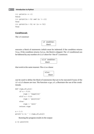
![9 1.2 Core Python
Loops
The while construct
while condition:
block
executes a block of (indented) statements if the condition is True. After execution
of the block, the condition is evaluated again. If it is still True, the block is exe-
cuted again. This process is continued until the condition becomes False. The else
clause
else:
block
can be used to define the block of statements that are to be executed if the condition
is false. Here is an example that creates the list [1, 1/2, 1/3, . . .]:
nMax = 5
n = 1
a = [] # Create empty list
while n nMax:
a.append(1.0/n) # Append element to list
n = n + 1
print(a)
The output of the program is
[1.0, 0.5, 0.33333333333333331, 0.25]
We met the for statement in Section 1.1. This statement requires a target and a
sequence over which the target loops. The form of the construct is
for target in sequence:
block
You may add an else clause that is executed after the for loop has finished.
The previous program could be written with the for construct as
nMax = 5
a = []
for n in range(1,nMax):
a.append(1.0/n)
print(a)
Here n is the target, and the range object [1, 2, . . . , nMax − 1] (created by calling
the range function) is the sequence.
Any loop can be terminated by the
break](https://image.slidesharecdn.com/21578834-250610045303-b34e4142/85/Numerical-Methods-In-Engineering-With-Python-3-3rd-Edition-Jaan-Kiusalaas-27-320.jpg)
![10 Introduction to Python
statement. If there is an else cause associated with the loop, it is not executed. The
following program, which searches for a name in a list, illustrates the use of break
and else in conjunction with a for loop:
list = [’Jack’, ’Jill’, ’Tim’, ’Dave’]
name = eval(input(’Type a name: ’)) # Python input prompt
for i in range(len(list)):
if list[i] == name:
print(name,’is number’,i + 1,’on the list’)
break
else:
print(name,’is not on the list’)
Here are the results of two searches:
Type a name: ’Tim’
Tim is number 3 on the list
Type a name: ’June’
June is not on the list
The
continue
statement allows us to skip a portion of an iterative loop. If the interpreter encounters
the continue statement, it immediately returns to the beginning of the loop without
executing the statements that follow continue. The following example compiles a
list of all numbers between 1 and 99 that are divisible by 7.
x = [] # Create an empty list
for i in range(1,100):
if i%7 != 0: continue # If not divisible by 7, skip rest of loop
x.append(i) # Append i to the list
print(x)
The printout from the program is
[7, 14, 21, 28, 35, 42, 49, 56, 63, 70, 77, 84, 91, 98]
Type Conversion
If an arithmetic operation involves numbers of mixed types, the numbers are
automatically converted to a common type before the operation is carried out.](https://image.slidesharecdn.com/21578834-250610045303-b34e4142/85/Numerical-Methods-In-Engineering-With-Python-3-3rd-Edition-Jaan-Kiusalaas-28-320.jpg)
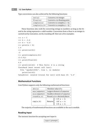
![12 Introduction to Python
It displays the prompt and then reads a line of input that is converted to a string. To
convert the string into a numerical value use the function
eval(string)
The following program illustrates the use of these functions:
a = input(’Input a: ’)
print(a, type(a)) # Print a and its type
b = eval(a)
print(b,type(b)) # Print b and its type
The function type(a) returns the type of the object a; it is a very useful tool in
debugging. The program was run twice with the following results:
Input a: 10.0
10.0 class ’str’
10.0 class ’float’
Input a: 11**2
11**2 class ’str’
121 class ’int’
A convenient way to input a number and assign it to the variable a is
a = eval(input(prompt))
Printing Output
Output can be displayed with the print function
print(object1, object2, . . .)
that converts object1, object2, and so on, to strings and prints them on the same line,
separated by spaces. The newline character ’n’ can be used to force a new line. For
example,
a = 1234.56789
b = [2, 4, 6, 8]
print(a,b)
1234.56789 [2, 4, 6, 8]
print(’a =’,a, ’nb =’,b)
a = 1234.56789
b = [2, 4, 6, 8]
The print function always appends the newline character to the end of a line.
We can replace this character with something else by using the keyword argument
end. For example,
print(object1, object2, ...,end=’ ’)
replaces n with a space.](https://image.slidesharecdn.com/21578834-250610045303-b34e4142/85/Numerical-Methods-In-Engineering-With-Python-3-3rd-Edition-Jaan-Kiusalaas-30-320.jpg)
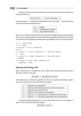
![14 Introduction to Python
Reading Data from a File
There are three methods for reading data from a file. The method
file object.read(n)
reads n characters and returns them as a string. If n is omitted, all the characters in
the file are read.
If only the current line is to be read, use
file object.readline(n)
which reads n characters from the line. The characters are returned in a string that
terminates in the newline character n. Omission of n causes the entire line to be
read.
All the lines in a file can be read using
file object.readlines()
This returns a list of strings, each string being a line from the file ending with the
newline character.
A convenient method of extracting all the lines one by one is to use the loop
for line in file object:
do something with line
As an example, let us assume that we have a file named sunspots.txt in the
working directory. This file contains daily data of sunspot intensity, each line having
the format (year/month/date/intensity), as follows:
1896 05 26 40.94
1896 05 27 40.58
1896 05 28 40.20
etc.
Our task is to read the file and create a list x that contains only the intensity. Since
each line in the file is a string, we first split the line into its pieces using the split
command. This produces a list of strings, such as[’1896’,’05’,’26’,’40.94’].
Then we extract the intensity (element [3] of the list), evaluate it, and append the
result to x. Here is the algorithm:
x = []
data = open(’sunspots.txt’,’r’)
for line in data:
x.append(eval(line.split()[3]))
data.close()](https://image.slidesharecdn.com/21578834-250610045303-b34e4142/85/Numerical-Methods-In-Engineering-With-Python-3-3rd-Edition-Jaan-Kiusalaas-32-320.jpg)
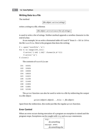
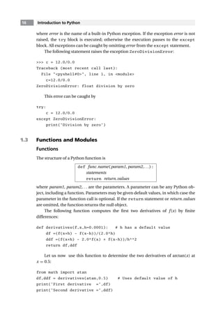
![17 1.3 Functions and Modules
Note that atan is passed to derivatives as a parameter. The output from the
program is
First derivative = 0.799999999573
Second derivative = -0.639999991892
The number of input parameters in a function definition may be left arbitrary.
For example, in the following function definition
def func(x1,x2,*x3)
x1 and x2 are the usual parameters, also called positional parameters, whereas x3
is a tuple of arbitrary length containing the excess parameters. Calling this function
with
func(a,b,c,d,e)
results in the following correspondence between the parameters:
a ←→ x1, b ←→ x2, (c,d,e) ←→ x3
The positional parameters must always be listed before the excess parameters.
If a mutable object, such as a list, is passed to a function where it is modified, the
changes will also appear in the calling program. An example follows:
def squares(a):
for i in range(len(a)):
a[i] = a[i]**2
a = [1, 2, 3, 4]
squares(a)
print(a) # ’a’ now contains ’a**2’
The output is
[1, 4, 9, 16]
Lambda Statement
If the function has the form of an expression, it can be defined with the lambda
statement
func name = lambda param1, param2,...: expression
Multiple statements are not allowed.
Here is an example:
c = lambda x,y : x**2 + y**2
print(c(3,4))
25](https://image.slidesharecdn.com/21578834-250610045303-b34e4142/85/Numerical-Methods-In-Engineering-With-Python-3-3rd-Edition-Jaan-Kiusalaas-35-320.jpg)
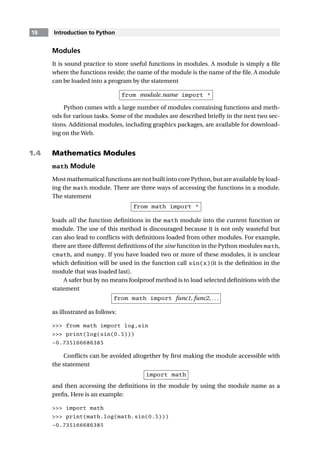
![19 1.4 Mathematics Modules
A module can also be made accessible under an alias. For example, the math
module can be made available under the alias m with the command
import math as m
Now the prefix to be used is m rather than math:
import math as m
print(m.log(m.sin(0.5)))
-0.735166686385
The contents of a module can be printed by calling dir(module). Here is how
to obtain a list of the functions in the math module:
import math
dir(math)
[’__doc__’, ’__name__’, ’acos’, ’asin’, ’atan’,
’atan2’, ’ceil’, ’cos’, ’cosh’, ’e’, ’exp’, ’fabs’,
’floor’, ’fmod’, ’frexp’, ’hypot’, ’ldexp’, ’log’,
’log10’, ’modf’, ’pi’, ’pow’, sign’, sin’, ’sinh’,
’sqrt’, ’tan’, ’tanh’]
Most of these functions are familiar to programmers. Note that the module in-
cludes two constants: π and e.
cmath Module
The cmath module provides many of the functions found in the math module, but
these functions accept complex numbers. The functions in the module are
[’__doc__’, ’__name__’, ’acos’, ’acosh’, ’asin’, ’asinh’,
’atan’, ’atanh’, ’cos’, ’cosh’, ’e’, ’exp’, ’log’,
’log10’, ’pi’, ’sin’, ’sinh’, ’sqrt’, ’tan’, ’tanh’]
Here are examples of complex arithmetic:
from cmath import sin
x = 3.0 -4.5j
y = 1.2 + 0.8j
z = 0.8
print(x/y)
(-2.56205313375e-016-3.75j)
print(sin(x))
(6.35239299817+44.5526433649j)
print(sin(z))
(0.7173560909+0j)](https://image.slidesharecdn.com/21578834-250610045303-b34e4142/85/Numerical-Methods-In-Engineering-With-Python-3-3rd-Edition-Jaan-Kiusalaas-37-320.jpg)
![20 Introduction to Python
1.5 numpy Module
General Information
The numpy module2
is not a part of the standard Python release. As pointed out ear-
lier, it must be installed separately (the installation is very easy). The module intro-
duces array objects that are similar to lists, but can be manipulated by numerous
functions contained in the module. The size of an array is immutable, and no empty
elements are allowed.
The complete set of functions in numpy is far too long to be printed in its entirety.
The following list is limited to the most commonly used functions.
[’complex’, ’float’, ’abs’, ’append’, arccos’,
’arccosh’, ’arcsin’, ’arcsinh’, ’arctan’, ’arctan2’,
’arctanh’, ’argmax’, ’argmin’, ’cos’, ’cosh’, ’diag’,
’diagonal’, ’dot’, ’e’, ’exp’, ’floor’, ’identity’,
’inner, ’inv’, ’log’, ’log10’, ’max’, ’min’,
’ones’, ’outer’, ’pi’, ’prod’ ’sin’, ’sinh’, ’size’,
’solve’, ’sqrt’, ’sum’, ’tan’, ’tanh’, ’trace’,
’transpose’, ’vectorize’,’zeros’]
Creating an Array
Arrays can be created in several ways. One of them is to use the array function to
turn a list into an array:
array(list,type)
Following are two examples of creating a 2 × 2 array with floating-point elements:
from numpy import array
a = array([[2.0, -1.0],[-1.0, 3.0]])
print(a)
[[ 2. -1.]
[-1. 3.]]
b = array([[2, -1],[-1, 3]],float)
print(b)
[[ 2. -1.]
[-1. 3.]]
Other available functions are
zeros((dim1,dim2),type)
which creates a dim1 × dim2 array and fills it with zeroes, and
ones((dim1,dim2),type)
which fills the array with ones. The default type in both cases is float.
2 NumPy is the successor of older Python modules called Numeric and NumArray. Their interfaces
and capabilities are very similar. Although Numeric and NumArray are still available, they are no
longer supported.](https://image.slidesharecdn.com/21578834-250610045303-b34e4142/85/Numerical-Methods-In-Engineering-With-Python-3-3rd-Edition-Jaan-Kiusalaas-38-320.jpg)
![21 1.5 numpy Module
Finally, there is the function
arange(from,to,increment)
which works just like the range function, but returns an array rather than a se-
quence. Here are examples of creating arrays:
from numpy import *
print(arange(2,10,2))
[2 4 6 8]
print(arange(2.0,10.0,2.0))
[ 2. 4. 6. 8.]
print(zeros(3))
[ 0. 0. 0.]
print(zeros((3),int))
[0 0 0]
print(ones((2,2)))
[[ 1. 1.]
[ 1. 1.]]
Accessing and Changing Array Elements
If a is a rank-2 array, then a[i,j] accesses the element in row i and column j,
whereas a[i] refers to row i. The elements of an array can be changed by assign-
ment as follows:
from numpy import *
a = zeros((3,3),int)
print(a)
[[0 0 0]
[0 0 0]
[0 0 0]]
a[0] = [2,3,2] # Change a row
a[1,1] = 5 # Change an element
a[2,0:2] = [8,-3] # Change part of a row
print(a)
[[ 2 3 2]
[ 0 5 0]
[ 8 -3 0]]
Operations on Arrays
Arithmetic operators work differently on arrays than they do on tuples and lists—the
operation is broadcast to all the elements of the array; that is, the operation is applied
to each element in the array. Here are examples:
from numpy import array
a = array([0.0, 4.0, 9.0, 16.0])](https://image.slidesharecdn.com/21578834-250610045303-b34e4142/85/Numerical-Methods-In-Engineering-With-Python-3-3rd-Edition-Jaan-Kiusalaas-39-320.jpg)
![22 Introduction to Python
print(a/16.0)
[ 0. 0.25 0.5625 1. ]
print(a - 4.0)
[ -4. 0. 5. 12.]
The mathematical functions available in numpy are also broadcast, as follows:
from numpy import array,sqrt,sin
a = array([1.0, 4.0, 9.0, 16.0])
print(sqrt(a))
[ 1. 2. 3. 4.]
print(sin(a))
[ 0.84147098 -0.7568025 0.41211849 -0.28790332]
Functions imported from the math module will work on the individual elements,
of course, but not on the array itself. An example follows:
from numpy import array
from math import sqrt
a = array([1.0, 4.0, 9.0, 16.0])
print(sqrt(a[1]))
2.0
print(sqrt(a))
Traceback (most recent call last):
.
.
.
TypeError: only length-1 arrays can be converted to Python scalars
Array Functions
There are numerous functions in numpy that perform array operations and other use-
ful tasks. Here are a few examples:
from numpy import *
A = array([[4,-2,1],[-2,4,-2],[1,-2,3]],float)
b = array([1,4,3],float)
print(diagonal(A)) # Principal diagonal
[ 4. 4. 3.]
print(diagonal(A,1)) # First subdiagonal
[-2. -2.]
print(trace(A)) # Sum of diagonal elements
11.0
print(argmax(b)) # Index of largest element
1
print(argmin(A,axis=0)) # Indices of smallest col. elements
[1 0 1]](https://image.slidesharecdn.com/21578834-250610045303-b34e4142/85/Numerical-Methods-In-Engineering-With-Python-3-3rd-Edition-Jaan-Kiusalaas-40-320.jpg)
![23 1.5 numpy Module
print(identity(3)) # Identity matrix
[[ 1. 0. 0.]
[ 0. 1. 0.]
[ 0. 0. 1.]]
There are three functions in numpy that compute array products. They are illus-
trated by the following program. For more details, see Appendix A2.
from numpy import *
x = array([7,3])
y = array([2,1])
A = array([[1,2],[3,2]])
B = array([[1,1],[2,2]])
# Dot product
print(dot(x,y) =n,dot(x,y)) # {x}.{y}
print(dot(A,x) =n,dot(A,x)) # [A]{x}
print(dot(A,B) =n,dot(A,B)) # [A][B]
# Inner product
print(inner(x,y) =n,inner(x,y)) # {x}.{y}
print(inner(A,x) =n,inner(A,x)) # [A]{x}
print(inner(A,B) =n,inner(A,B)) # [A][B_transpose]
# Outer product
print(outer(x,y) =n,outer(x,y))
print(outer(A,x) =n,outer(A,x))
print(outer(A,B) =n,outer(A,B))
The output of the program is
dot(x,y) =
17
dot(A,x) =
[13 27]
dot(A,B) =
[[5 5]
[7 7]]
inner(x,y) =
17
inner(A,x) =
[13 27]
inner(A,B) =
[[ 3 6]
[ 5 10]]
outer(x,y) =](https://image.slidesharecdn.com/21578834-250610045303-b34e4142/85/Numerical-Methods-In-Engineering-With-Python-3-3rd-Edition-Jaan-Kiusalaas-41-320.jpg)
![24 Introduction to Python
[[14 7]
[ 6 3]]
outer(A,x) =
[[ 7 3]
[14 6]
[21 9]
[14 6]]
Outer(A,B) =
[[1 1 2 2]
[2 2 4 4]
[3 3 6 6]
[2 2 4 4]]
Linear Algebra Module
The numpy module comes with a linear algebra module called linalg that contains
routine tasks such as matrix inversion and solution of simultaneous equations. For
example,
from numpy import array
from numpy.linalg import inv,solve
A = array([[ 4.0, -2.0, 1.0],
[-2.0, 4.0, -2.0],
[ 1.0, -2.0, 3.0]])
b = array([1.0, 4.0, 2.0])
print(inv(A)) # Matrix inverse
[[ 0.33333333 0.16666667 0. ]
[ 0.16666667 0.45833333 0.25 ]
[ 0. 0.25 0.5 ]]
print(solve(A,b)) # Solve [A]{x} = {b}
[ 1. , 2.5, 2. ]
Copying Arrays
We explained earlier that if a is a mutable object, such as a list, the assignment state-
ment b = a does not result in a new object b, but simply creates a new reference to
a, called a deep copy. This also applies to arrays. To make an independent copy of an
array a, use the copy method in the numpy module:
b = a.copy()
Vectorizing Algorithms
Sometimes the broadcasting properties of the mathematical functions in the numpy
module can be used to replace loops in the code. This procedure is known as](https://image.slidesharecdn.com/21578834-250610045303-b34e4142/85/Numerical-Methods-In-Engineering-With-Python-3-3rd-Edition-Jaan-Kiusalaas-42-320.jpg)
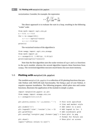
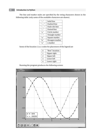
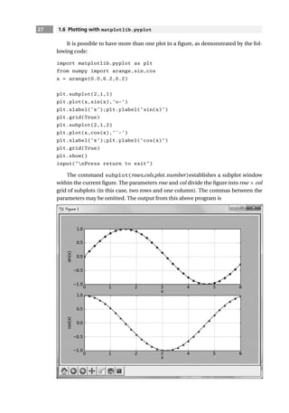

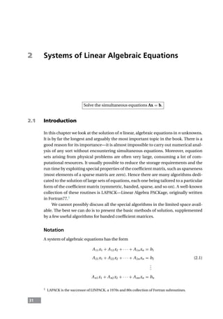
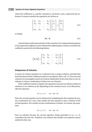
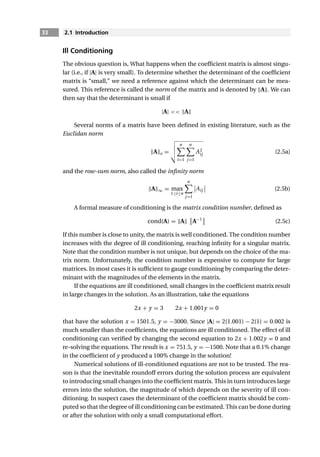
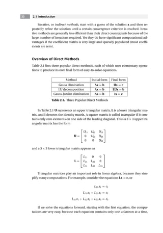

![Hamblen put it. It was typed in pencil. I think he meant is printed in
pencil.
I asked him to immediately set about to obtain copies of that, as
I was leaving town, and to get a copy of the message, and to do
that it would be necessary for him to see Mr. Pirtle, our bookkeeping
manager, and to get the message, put it in an envelope, and address
it to my personal attention while I was in Kansas City.
Mr. Liebeler. Did Mr. Hamblen tell you anything about what the
message said or to whom it was addressed at this first conversation?
Mr. Wilcox. No, he didn't. We left for Kansas City and was there
over the Thanksgiving holidays.
Mr. Liebeler. You and your family?
Mr. Wilcox. Yes. And while there, this article appeared in the
Kansas City Star, their evening paper; very much the same story as
appeared in the Dallas Times Herald.
Mr. Liebeler. I show you a copy of a clipping which purports to
have appeared in the Dallas Times Herald on November 30, 1963. I
ask you if this tells a story similar to the report you saw in the
Kansas City Star?
Mr. Wilcox. Yes, same story.
Mr. Liebeler. We will mark this clipping as Exhibit 3002 on the
deposition of Laurance R. Wilcox, at Dallas, Tex., March 31, 1964. I
have initialed the clipping in question, Mr. Wilcox, and ask you to do
the same.
Mr. Wilcox. [Initials.] Immediately when I read this story in the
Kansas City paper I recognized it as being the same story that Mr.
Hamblen had told me just a couple of days before in my office.
We returned to Dallas Sunday, and immediately on my return to
the office Monday——
Mr. Liebeler. Monday, I suggest would have been December 2,
1963?](https://image.slidesharecdn.com/21578834-250610045303-b34e4142/85/Numerical-Methods-In-Engineering-With-Python-3-3rd-Edition-Jaan-Kiusalaas-59-320.jpg)
![Mr. Liebeler. I mark that letter as Exhibit 3003, on the deposition
of Mr. Laurance R. Wilcox, at Dallas, Tex., March 31, 1964. I have
initialed the copy in question, Mr. Wilcox, and would like to have you
do the same thing if you would.
Mr. Wilcox. [Initials.]
Mr. Liebeler. Before we go on, I call your attention to the fact
that this letter of December 3, 1963, starts out by saying This is to
supplement my report of December 2 in connection with newspaper
article regarding messages and money order to Ruby or Oswald.
Do you have a copy of your report of December 2, referred to in
Exhibit 3003?
Mr. Wilcox. Yes, sir.
Mr. Liebeler. May we mark that as Exhibit No. 3004 on the
deposition of Mr. Laurance R. Wilcox, Dallas, Tex., March 31, 1964?
Mr. Wilcox. [Hands document to attorney.]
Mr. Liebeler. I have initialed Exhibit No. 3004 and you have done
likewise, have you not?
Mr. Wilcox. Yes, sir.
Mr. Liebeler. You had just indicated that you had talked to Mr.
Hamblen upon your return concerning the newspaper story. Would
you tell us what happened next?
Mr. Wilcox. I asked Mr. Hamblen if he had obtained the message
from the bookkeeping department as I had requested he do, and he
stated that he had not found it and did not have it and it wasn't
available.
On December 9, Mr. Semingsen, vice president of Western
Union, was at my office, and at this time we interviewed several
employees for the purpose of finding out if any of them could recall
having seen Oswald in our office. We also discussed the Ruby money
orders.](https://image.slidesharecdn.com/21578834-250610045303-b34e4142/85/Numerical-Methods-In-Engineering-With-Python-3-3rd-Edition-Jaan-Kiusalaas-61-320.jpg)
![Mr. Wilcox. Yes. This statement was obtained at the time I
discussed the matter with Mr. Hamblen on December 2, Monday.
That was this statement.
Mr. Liebeler. That visit with Mr. Hamblen is described in Exhibit
No. 3003, your letter to Mr. Semingsen on December 3, 1963, is that
correct?
Mr. Wilcox. Yes, sir.
Mr. Liebeler. And the statement of Mr. Hamblen, dated December
2, 1963, was obtained at that time? That time being the first time
that you talked to Mr. Hamblen after this matter appeared in the
newspapers; is that correct?
Mr. Wilcox. Yes.
Mr. Liebeler. Do you have the original of Mr. Hamblen's statement
of December 2, 1963?
Mr. Wilcox. I can't find it in my file. I am wondering if it was sent
to Mr. Semingsen's file, but we have gone through that.
Mr. Liebeler. I show you a thermofax copy that has been provided
to us, and ask you if that is an accurate copy of the original
statement?
Mr. Wilcox. Yes. That was made in our office on the thermofax
machine.
Mr. Liebeler. Let us mark the thermofax copy of the statement of
Mr. C. A. Hamblen to Mr. Wilcox dated December 2, 1963, as Exhibit
3005 on the deposition of Mr. Laurance R. Wilcox, at Dallas, Tex., on
March 31, 1964.
I have initialed Exhibit 3005, Mr. Wilcox. Will you do the same?
Mr. Wilcox. [Initials.]
Mr. Liebeler. Does the statement of Mr. Hamblen, Exhibit No.
3005, accurately reflect the conversation which you had with him on
December 2, 1963?](https://image.slidesharecdn.com/21578834-250610045303-b34e4142/85/Numerical-Methods-In-Engineering-With-Python-3-3rd-Edition-Jaan-Kiusalaas-63-320.jpg)
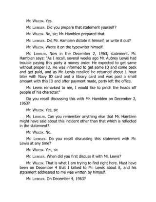
![Mr. Wilcox. On December 4, 1963.
Mr. Liebeler. Do you have a copy of that statement?
Mr. Wilcox. Yes, sir.
Mr. Liebeler. Could we mark that as Exhibit No. 3006 on the
deposition of Laurance R. Wilcox, at Dallas, Tex., March 31, 1964?
In this case you have actually provided me the original of Mr.
Lewis' statement, is that correct?
Mr. Wilcox. Yes, sir.
Mr. Liebeler. I have initialed Exhibit No. 3006 and would like to
have you do the same, if you would.
Mr. Wilcox. [Initials.]
Mr. Liebeler. Mr. Lewis' statement refers to that portion of Mr.
Hamblen's statement, dated December 2, 1963, which we just read,
does it not?
Mr. Wilcox. Yes, sir.
Mr. Liebeler. And Mr. Lewis says that he does recall the difficulty
he had paying a small money order to a gentleman who struck him
as being a feminine type of person, but says he cannot remember
the name of that person; is that correct?
Mr. Wilcox. Yes, sir.
Mr. Liebeler. Do you remember discussing that with Mr. Lewis to
any extent other than as reflected on this statement?
Mr. Wilcox. Yes, sir.
Mr. Liebeler. Could you tell us what you said and what Mr. Lewis
said about this?
Before you tell us what was said, this discussion that you are
referring to was held on December 4, 1963, or some other time?
Mr. Wilcox. Yes, sir; at that time.](https://image.slidesharecdn.com/21578834-250610045303-b34e4142/85/Numerical-Methods-In-Engineering-With-Python-3-3rd-Edition-Jaan-Kiusalaas-65-320.jpg)
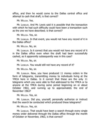
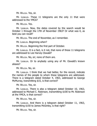
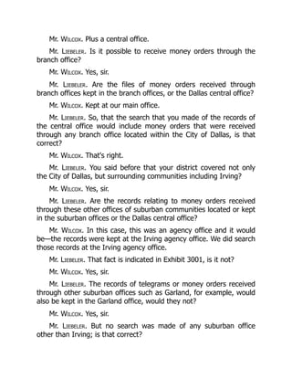
![Mr. Wilcox. That's right.
Mr. Liebeler. Mr. Semingsen's memorandum also indicates that a
search was made of the files in Fort Worth and in New Orleans, but
you have no direct personal knowledge of what happened at those
offices, do you?
Mr. Wilcox. No, sir.
Mr. Liebeler. We also have here a statement from Mr. Hamblen
dated December 5, 1963. Do you have the original of that
statement?
Mr Wilcox. Yes; I do have.
Mr. Liebeler. We will mark the original as Exhibit No. 3007 on the
deposition of Laurance R. Wilcox, at Dallas, Tex., March 31, 1963.
I have initialed Exhibit No. 3007, Mr. Wilcox, and I would like you
do the same.
Mr. Wilcox. [Initials.]
Mr. Liebeler. This statement was apparently taken on December
5, 1963. Do you recall the circumstances under which it was given?
Mr. Wilcox. This was following a meeting and discussion that we
held on December 4, at which time we discussed the money orders
and messages with Mr. Hamblen, Mrs. McClure, and Mr. Lewis.
Mr. Liebeler. Who was present at this discussion other than the
individuals you just mentioned and yourself?
(Mr. Wilcox phoned his office re: correct date of meeting.)
Mr. Wilcox. I did hold this meeting.
Mr. Liebeler. Let the record indicate that Mr. Wilcox has just
conferred telephonically with Mr. Semingsen and wishes now to
clarify the statements concerning the time on which certain meetings
were held with the employees.
Mr. Wilcox. I did hold the meetings with these people on
December 4, and did obtain these statements, including the](https://image.slidesharecdn.com/21578834-250610045303-b34e4142/85/Numerical-Methods-In-Engineering-With-Python-3-3rd-Edition-Jaan-Kiusalaas-75-320.jpg)
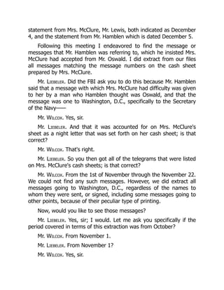
![Mr. Liebeler. You picked that period because Mr. Hamblen said
that he thought the event occurred about 10 days prior to the
assassination; is that correct?
Mr. Wilcox. That's right. Now, I think you have the only
thermofax of Mrs. McClure's. Would you want the original?
Mr. Liebeler. Yes; I do want to mark the original statement of
Mrs. McClure, dated December 4, 1963, which has been previously
referred to by Mr. Wilcox. I will mark it as Exhibit 3008 on the
deposition of Mr. Laurance R. Wilcox at Dallas, Tex., on March 31,
1964.
I have initialed that exhibit, Mr. Wilcox, and would like to have
you do the same.
Mr. Wilcox. [Initials.]
Mr. Liebeler. Who prepared Mrs. McClure's statement?
Mr. Wilcox. Mrs. McClure wrote that.
Mr. Liebeler. She typed it on the typewriter herself?
Mr. Wilcox. Yes, sir.
Mr. Liebeler. Were you present at the time she prepared it?
Mr. Wilcox. Yes, sir.
Mr. Liebeler. Did you discuss these incidents with her prior to the
statement?
Mr. Wilcox. Only during the course of the meeting that she
attended in my office.
Mr. Liebeler. During the course of that time, Mrs. McClure
indicated to you, did she not, that she had no recollection of any of
the events described by Mr. Hamblen concerning the message
allegedly sent to Washington, D.C.?
Mr. Wilcox. That's right.](https://image.slidesharecdn.com/21578834-250610045303-b34e4142/85/Numerical-Methods-In-Engineering-With-Python-3-3rd-Edition-Jaan-Kiusalaas-77-320.jpg)
![Mr. Liebeler. Let's mark these telegrams as Exhibits 3009 through
3014. I have initialed each one of them and would like to have you
do the same. I have not indicated on each one of them in detail. It is
on your deposition and on the dates, as I have on the others, but
that fact will appear from the record.
Mr. Wilcox. [Initials.]
Mr. Liebeler. You have now provided me with six telegrams,
cables which have been marked for identification as Exhibits 3009
through 3014, and it is my understanding that these telegrams and
cables were all shown to Mr. Hamblen and he was unable to identify
any of them as answering the description of the telegram or
cablegram with which Mrs. McClure had had difficulty, and which Mr.
Hamblen thought had been sent by a person resembling Lee Harvey
Oswald, is that correct?
Mr. Wilcox. That's right.
Mr. Liebeler. And a thorough search of the files along the lines
that you have previously indicated was unable to produce any other
telegrams even remotely falling into the category described by Mr.
Hamblen; i.e., a telegram to Washington, D.C. or in a peculiar hand
script such as described by Mr. Hamblen to any destination, whether
it be Washington or otherwise; is that correct?
Mr. Wilcox. That's right.
Mr. Liebeler. Now, you have provided me with a letter from
yourself to Mr. Semingsen, dated December 6, 1963, which we will
mark as Exhibit 3015, on deposition of Laurance R. Wilcox, at Dallas,
Tex., March 31, 1964. I have initialed that exhibit and ask you to do
the same, sir.
Mr. Wilcox. [Initials.]
Mr. Liebeler. And ask you if you prepared the original of that
letter on or about December 6, 1963?
Mr. Wilcox. That's right.](https://image.slidesharecdn.com/21578834-250610045303-b34e4142/85/Numerical-Methods-In-Engineering-With-Python-3-3rd-Edition-Jaan-Kiusalaas-78-320.jpg)
![Mr. Liebeler. You sent the original of it to Mr. Semingsen, did you
not?
Mr. Wilcox. Yes, sir; that's right.
Mr. Liebeler. And the letter accurately sets forth the events
preceding that date which we have been discussing here, does it
not?
Mr. Wilcox. Yes, sir.
Mr. Liebeler. You have also provided me with a copy of a letter
from yourself to Mr. Semingsen, dated December 9, 1963, to which
is attached the original of statement from Mrs. Betty Bedwell, dated
December 6, 1963, and A. I. English, dated December 6, 1963. I
notice that Mr. English's statement is not signed.
Mr. Wilcox. [Signs.]
Mr. Liebeler. And I ask you if the original of it was signed at the
time you received it?
Mr. Wilcox. No, sir; he just signed this on the typewriter to me.
Mr. Liebeler. No; he did not himself sign it?
Mr. Wilcox. No.
Mr. Liebeler. You have indicated below that it was in effect signed
by Mr. English when he delivered it to you?
Mr. Wilcox. Yes, sir.
Mr. Liebeler. Also attached is a statement of Miss Bess Mildred
Francis, dated December 9, 1963. Also attached is a statement of
Doyle E. Lane, dated December 9, 1963; and one of Mr. E. T. Pirtle,
dated December 6, 1963; and one of Ward Townsley dated
December 6, 1963. Did you receive those statements from the
individuals thus described?
Mr. Wilcox. Yes, sir.
Mr. Liebeler. We have marked the letter described above,
together with the attachments just described as Exhibit 3016 on the](https://image.slidesharecdn.com/21578834-250610045303-b34e4142/85/Numerical-Methods-In-Engineering-With-Python-3-3rd-Edition-Jaan-Kiusalaas-79-320.jpg)
![deposition of Mr. Laurance R. Wilcox at Dallas, Tex., on March 31,
1964. I have initialed the first page of that exhibit and would like to
have you do the same.
Mr. Wilcox. [Initials.]
Mr. Liebeler. Did you send the original of your letter dated
December 9, 1963, to Mr. Semingsen on or about that date?
Mr. Wilcox. Yes, sir.
Mr. Liebeler. The statements made in that letter are true and
correct to the best of your knowledge, are they not?
Mr. Wilcox. Yes, sir.
Mr. Liebeler. You have also given me the original of a statement
dated December 6, 1963, of Mr. Doyle E. Lane. Was that also
attached to your letter of December 9, 1963, to Mr. Semingsen?
Mr. Wilcox. No, sir.
Mr. Liebeler. Did you receive yourself from Mr. Lane the
statement just described?
Mr. Wilcox. Yes, sir.
Mr. Liebeler. Let me mark it as Exhibit 3017 on this deposition.
Would you initial the statement of Mr. Lane which we have
marked 3017?
Mr. Wilcox. Yes, sir. [Initials.]
Mr. Liebeler. Thank you.
You previously testified, Mr. Wilcox, that you had a meeting on
or about December 4, 1963, with Mr. Hamblen, Mrs. McClure, and
Mr. Lewis in regard to the meeting we have been discussing, and
you also testified that you thought you had an additional meeting on
December 9, 1963, at which Mr. Semingsen was present. Would you
care to elaborate on that?](https://image.slidesharecdn.com/21578834-250610045303-b34e4142/85/Numerical-Methods-In-Engineering-With-Python-3-3rd-Edition-Jaan-Kiusalaas-80-320.jpg)