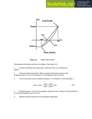
Download to read offline


![F 4
( ) =
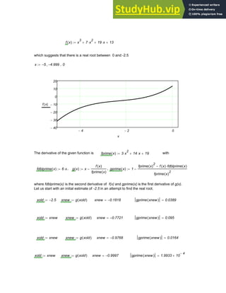
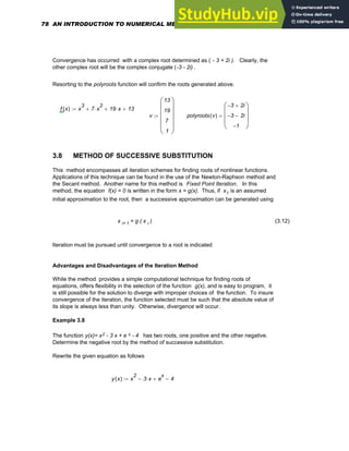
F <-This does not work
F x
( ) x
2
4
−
:=
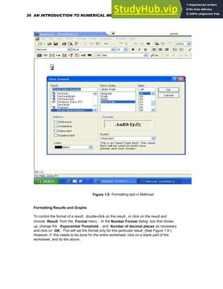
1.6 GRAPHICS
It has been demonstrated that Mathcad can be used as a calculator and as an equation solver.
It can also be used as a versatile visualization tool that supports a full set of plot types, an
animation facility, as well as simple image processing.
1.7 GRAPHING OF FUNCTIONS AND PLOTTING OF DATA
To create a plot in Mathcad, type the expression you would like to plot, say t
9
. Then click the
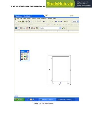
graphing button on your palette bar (See Figure 1.2 ) to bring up the graphing palette and click
the upper left button for an XY plot. Click outside the graph or press [Enter] to see the result:
4
− 2
− 0 2 4
1
− 10
5
×
5
− 10
4
×
0
5 10
4
×
1 10
5
×
t
9
t
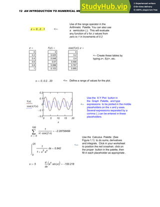
Parametric plots can also be done easily . .
1
− 0.5
− 0 0.5 1
1
−
0.5
−
0
0.5
1
sin 5 t
⋅
( )
cos 7 t
⋅
( )
Chapter 1: Basics of Mathcad 5](https://image.slidesharecdn.com/anintroductiontonumericalmethodsusingmathcadmathcadrelease14-230805170449-0ea94cc2/85/AN-INTRODUCTION-TO-NUMERICAL-METHODS-USING-MATHCAD-Mathcad-Release-14-15-320.jpg)


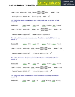
![Several mathcad palettes can be found on the palette strip at the top of the window that give
access to Mathcad's mathematical operators. A click in your worksheet will place a red
crosshair cursor. Math operators can now be placed in the worksheet via these palettes. To
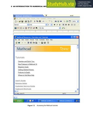
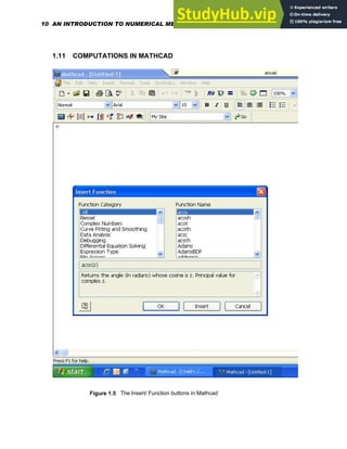
access Mathcad's built-in functions, go to the Insert menu as shown in Figure 1.5, and
select Function , or click on the Insert Function button on the toolbar
.
EXAMPLES
In the following examples, the number of decimal places required may be put in by choosing
Result from the Format menu and then selecting Number Format.
The red crosshair
Use the Arithmetic Palette (See Figure 1.1)
, and type = to obtain the answer. The basic
operations are +, -, *, and / which are
available on the keyboard .
2.645 10
8
⋅
30007
5
5
6
+
1.0426928428 10
7
−
×
= <--
<- Examples of built-in functions (See
Figure 1.5)
log 1768.985
( ) sin
4
79
π
⋅
⎛
⎜
⎝
⎞
⎟
⎠
⋅ 0.514
=
14.95 5.7i
( )
+
[ ]
3
e
6 5i
−
+ 1.999 10
3
× 4.024i 10
3
×
+
= <-- Complex numbers.
Use of units- Choose Unit from
the Insert menu (See Figure 1.5)
<--- .
7600 km
⋅
1 hr
⋅
2.11 10
3
× m s
1
−
⋅
=
Use of := by typing a colon
character or using the
Arithmetic Palette
a 8
:= a
3 a
4
+ 513.414
= <----
f x
( )
sin x
( )
a
x
6
+
:= f 37
( ) 0.045
−
= <-- Use of a defined function
Chapter 1: Basics of Mathcad 11](https://image.slidesharecdn.com/anintroductiontonumericalmethodsusingmathcadmathcadrelease14-230805170449-0ea94cc2/85/AN-INTRODUCTION-TO-NUMERICAL-METHODS-USING-MATHCAD-Mathcad-Release-14-21-320.jpg)

![Controlling Calculation and The Status Line
The calculation mode, whether manual or automatic, is a property saved in your worksheet and
template files. Mathcad starts in the automatic mode and all calculations and results are updated
automatically. The word " Auto " can be seen in the message line at the bottom of the Mathcad
window. This line provides status alerts, tips, keyboard shortcuts, and other helpful information
along with the calculation status of the worksheet . Here, "auto" refers to the automatic
mode , in which Mathcad automatically recalculates any math expressions when changes in the
worksheet are made. When "WAIT" appears on the status line, the cursor changes to a flashing
lightbulb, indicating that Mathcad is still completing computations. Besides giving the page
number of the current worksheet, the message line will also indicate whether the Caps Lock or
the Num Lock key is depressed on your keyboard. In manual mode, Mathcad does not
compute or show results until recalculation is specifically requested. However, while in manual
mode, Mathcad does keep track of pending computations . Once a change is made that requires
recalculation, the word " Calc " appears on the status line to indicate to the user that the results
being displayed are not correct and that recalculation is necessary to ensure accuracy. The
screen can then be updated by going to the Tools menu and choosing Calculate and then
Calculate Now . Alternatively, click = on the Standard toolbar or press [F9]. To force
Mathcad to recalculate all equations in the worksheet, go to the Tools menu and choose
Calculate and then Calculate Worksheet .
1.13 MATHCAD REGIONS
Mathcad allows you to enter equations, text and graphs as separate objects anywhere in the
worksheet and each equation, text paragraph or plot is considered a region. A region can be
selected by clicking in math or text in your worksheet, after which it is indicated by a thin
rectangle around it. Moving the cursor to one of the edges of the region, will change it to a
small hand with which the region can be moved to anywhere in the worksheet. While clicking
in the math region will bring blue selecting lines under the material selected, clicking in a text
region will bring black boxes to each corner and the middle of each line. With these boxes
text regions can be resized as needed. To add a border around a region or regions, select the
region(s), then right-click and choose Properties from the menu. Then click on the Display tab
and check the box next to " Show Border ".
A math region looks like: A text region looks like:
x 1535.56
:= What is shown on the left was
created by typing
x:1535.56
Chapter 1: Basics of Mathcad 15](https://image.slidesharecdn.com/anintroductiontonumericalmethodsusingmathcadmathcadrelease14-230805170449-0ea94cc2/85/AN-INTRODUCTION-TO-NUMERICAL-METHODS-USING-MATHCAD-Mathcad-Release-14-25-320.jpg)


![f x
( ) x 6
+
( ) x
3
5
−
( )
⋅
:=
Type
f(x):x+6[Spacebar]*(x^3[Spacebar]-5)
Example 2
To create
f x
( ) x 765 x
6 4
−
( )
⋅
+
:=
Type
f(x):x+765*(x^6-4)
The exponent operator is called a sticky operator because unless you get out by pressing
[Spacebar] , your keystrokes will "stick" to the exponent . This stickiness applies to
exponents, square roots, subscripts, and division.
Example 3
To create the expression
x
7
675
+
780
Type
x^7[Spacebar] <-- Puts x 7 in blue editing lines
+675[Spacebar] <-- Puts the whole equation in the editing lines
/780[Enter] <-- Expression is complete
Example 4
To create
22 AN INTRODUCTION TO NUMERICAL METHODS USING MATHCAD](https://image.slidesharecdn.com/anintroductiontonumericalmethodsusingmathcadmathcadrelease14-230805170449-0ea94cc2/85/AN-INTRODUCTION-TO-NUMERICAL-METHODS-USING-MATHCAD-Mathcad-Release-14-32-320.jpg)
![x
7 675
780
+
do the same as above but without pressing the spacebar after +675
Example 5
To create
x
17
t
7
450
type
x^17/t^7[Spacebar][Spacebar][Spacebar]/450
Editing Expressions
The equation editor functions very much like a text editor and goes from left to right. Most
problems dealing with editing equations stem from working with operators. Although Mathcad
automatically inserts parentheses wherever necessary, the Mathcad user must put in
parentheses himself in accordance with his own judgement to give clarity to expressions .
When expressions become complicated, it is definitely preferable to work with smaller and
more manageable subexpressions within them. The reader is referred to Chapter 4 of the
Mathcad 14 User's Guide for a detailed discussion on Editing Expressions. This can be
accessed by choosing Tutorials from the Help menu.
1.19 DEFINING RANGE VARIABLES
To assign a range of values to a variable x going from 0 to 30, say, with an increment
of 3, type
x:0,3;30
The result on the screen will be
x 0 3
, 30
..
:=
To evaluate a function f(x) for x= 0 to 7 with an increment of 1, type
x:0;7 f(x):x^5[Spacebar]-6*x^3[Spacebar]+9
Chapter 1: Basics of Mathcad 23](https://image.slidesharecdn.com/anintroductiontonumericalmethodsusingmathcadmathcadrelease14-230805170449-0ea94cc2/85/AN-INTRODUCTION-TO-NUMERICAL-METHODS-USING-MATHCAD-Mathcad-Release-14-33-320.jpg)

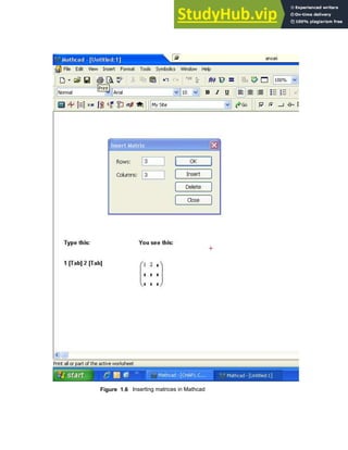
![To create a vector V , click in a blank space, Choose Matrix from the Insert menu (See
Figure 1.6 ) or click on the button inside the Vector and Matrix Palette . Then, fill in the
appropriate number of rows and columns, click on Insert and finally fill in the placeholders with
given values. To move from placeholder to placeholder inside the vector, use [Tab] or click on
the appropriate placeholder to select it
V
7
8
9
⎛
⎜
⎜
⎜
⎝
⎞
⎟
⎟
⎟
⎠
:=
To access a particular element of a vector, use the subscript operator , which can be
created by typing a left square bracket ( [ ), or by using the Xn button in the Matrix
Palette .
In Mathcad , by default the first element has the index 0. Type
V[0=
to see on the screen
V0 7
=
The next two elements will have indices 1 and 2 Thus typing V[1= and V[2= will
produce on the screen
V1 8
= V2 9
=
In order to obtain all the elements of the vector at the same time, the index can be defined
as a range variable as shown below::
i 0 2
..
:= giving Vi
7
8
9
=
<--- Type V[i=
The elements of a vector can also be used as the arguments of a function as shown below.
Define a function f(x) as.
f x
( ) sin 2 x
⋅
( ) cos 3 x
⋅
( )
+
:=
Let a vector V be a three-element vector as given below
26 AN INTRODUCTION TO NUMERICAL METHODS USING MATHCAD](https://image.slidesharecdn.com/anintroductiontonumericalmethodsusingmathcadmathcadrelease14-230805170449-0ea94cc2/85/AN-INTRODUCTION-TO-NUMERICAL-METHODS-USING-MATHCAD-Mathcad-Release-14-36-320.jpg)
![v
1.3
2.6
−
7.9
⎛
⎜
⎜
⎜
⎝
⎞
⎟
⎟
⎟
⎠
:=
Then, typing i:0;2 and then f(v[i)= will show the following on the screen
i 0 2
..
:= f vi
( )
-0.21
0.937
0.046
=
The Vector and Matrix Palette contains most of the common matrix and vector operators.
These are listed below.
Operation Keystroke
Palette
Button Display
Dot product [Shift]8 v w
⋅ Displays like scalar
multiplication.
Cross product [Ctrl]8 v w
×
Determinant | M
Column [Ctrl]6 M
2
〈 〉
Returns the 2nd
column of M.
There is also a wide range of built-in functions in Mathcad that return information about the
size of an array and its elements. For a given matrix [M], various pieces of information can
be generated as shown below.
M
9
4
12
10
5
13
11
7
14
⎛
⎜
⎜
⎜
⎝
⎞
⎟
⎟
⎟
⎠
:=
Chapter 1: Basics of Mathcad 27](https://image.slidesharecdn.com/anintroductiontonumericalmethodsusingmathcadmathcadrelease14-230805170449-0ea94cc2/85/AN-INTRODUCTION-TO-NUMERICAL-METHODS-USING-MATHCAD-Mathcad-Release-14-37-320.jpg)
![Number of columns: cols M
( ) 3
= Number of rows: rows M
( ) 3
=
Largest value in matrix: max M
( ) 14
= Determinant of matrix: M 3
=
Eigenvalues of a matrix: eigenvals M
( )
28.768
0.176
−
0.592
−
⎛
⎜
⎜
⎜
⎝
⎞
⎟
⎟
⎟
⎠
=
1.21 CREATING GRAPHS
To create an x-y plot, choose Graph/ X-Y Plot from the Insert Menu as shown in Figure
1.7. Press [Enter] and fill in the placeholders on the x and y axes. Alternatively, type an
expression depending on one variable such as: sin(x) + cos (3x) and click on the X-Y Plot
button on the Graph toolbar . The resulting plot will be
x 10
− 9.9
−
, 10
..
:=
10
− 5
− 0 5 10
2
−
1
−
1
2
sin x
( ) cos 3 x
⋅
( )
+
x
28 AN INTRODUCTION TO NUMERICAL METHODS USING MATHCAD](https://image.slidesharecdn.com/anintroductiontonumericalmethodsusingmathcadmathcadrelease14-230805170449-0ea94cc2/85/AN-INTRODUCTION-TO-NUMERICAL-METHODS-USING-MATHCAD-Mathcad-Release-14-38-320.jpg)

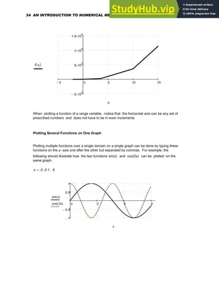
![Using Range Variables to Plot a Function
The range of values being plotted on the x-axis must, in general, be specified. If this range is
not prescibed by you, Mathcad will choose a default range for the dependent variable. For
example, let us plot
f x
( ) x
3
8 x
2
⋅
+ 9 x
⋅
+ 14
+
:=
The graph of this function over the range x= 0 to x= 6 can be accomplished as follows.
x 0 1
, 6
..
:= f x
( ) x
3
8 x
2
⋅
+ 9 x
⋅
+ 14
+
:=
Now create the plot by clicking in the worksheet window. Type @ to create the x-y plot, type
x in the middle placeholder on the horizontal axis and type f(x) in the middle placeholder
on the vertical axis. Press [Enter] . The following graph should then appear on the screen.
0 2 4 6
0
200
400
600
f x
( )
x
The plot generated above does not seem to be very smooth. In order to obtain a smoother
trace, change the definition of x to x 0 0.1
, 6
..
:= . The smaller step enables Mathcad to
calculate more points. This will make the plot a lot smoother (see graph below ) because now
there are more points or dots being connected together.
Formatting of an x-y plot can be accomplished as follows. Double-click on it or choose Graph
from the Format menu to open up a dialog box. This dialog box will allow several options in
terms of grid lines, legends, trace types, markers, colors, axis limits etc.
30 AN INTRODUCTION TO NUMERICAL METHODS USING MATHCAD](https://image.slidesharecdn.com/anintroductiontonumericalmethodsusingmathcadmathcadrelease14-230805170449-0ea94cc2/85/AN-INTRODUCTION-TO-NUMERICAL-METHODS-USING-MATHCAD-Mathcad-Release-14-40-320.jpg)
![x 0 0.1
, 6
..
:=
0 2 4 6
200
400
600
f x
( )
x
Plotting a Vector of Data Points
Let us say that we need to plot a vector of data points called Temp , which is the rising
outside temperature on different days of a week in a summer month. This vector which will
have 7 rows and 1 column can be created using the Matrix command on the Insert menu.
Temp
78
82
84
86
88
90
92
⎛
⎜
⎜
⎜
⎜
⎜
⎜
⎜
⎜
⎜
⎝
⎞
⎟
⎟
⎟
⎟
⎟
⎟
⎟
⎟
⎟
⎠
:=
This data can be graphed by making the horizontal axis an index variable or a vector with
the same number of elements as the vector Temp . Define the index i as:
i 0 6
..
:=
Create your plot by typing [@] and typing in
Temp[i
Chapter 1: Basics of Mathcad 31](https://image.slidesharecdn.com/anintroductiontonumericalmethodsusingmathcadmathcadrelease14-230805170449-0ea94cc2/85/AN-INTRODUCTION-TO-NUMERICAL-METHODS-USING-MATHCAD-Mathcad-Release-14-41-320.jpg)


![ε xmidi 1
+ xmidi
−
= (3.1)
(3.2)
εrel
xmidi 1
+ xmidi
−
xmidi 1
+
100
⋅
= percent
where xmid i+1 and xmid i are the midpoints in the current and previous iterations. While,
in general, the relative error should not be greater than 5 %, an error of 0.01 % is the
largest that is tolerable for some classes of problems, that require immense precision.
The true error , ε True , is an indicator of the real accuracy of a solution and can be
evaluated only if the true solution, x True , is known. It is defined as
εTrue
xTrue xmidi
−
xTrue
100
⋅
= (3.3)
Calculation of the true error clearly requires knowledge of the true solution, which, in general,
will not be known to us. Therefore, the quantity ε rel may have to be mostly used to
determine the error associated with a solution process.
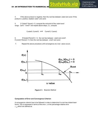
Advantages and Disadvantages of Bisection
While Bisection is a simple, robust technique for finding one root in a given interval, when
the root is known to exist and it works even for non-analytic functions, its convergence
process is generally slow, making it a somewhat inefficient procedure.
Sometimes, a singularity may be identified as if it were a root, since the method does not
distinguish between roots and singularities, at which the function would go to infinity.
Therefore, as the method proceeds, a check must be made to see if the absolute value of
[f(xend)-f(xstart)], in fact, converges to zero. If this quantity diverges, the method is chasing
a singularity rather than a root .
When there are multiple roots, Bisection is not a desirable technique to use, since the
function may not change signs at points on either side of the roots. Therefore, a graph of
the function must first be drawn before proceeding to do the calculations.
Example 3.1
Obtain a root of f(x) in the range of 4 < x < 20
f(x)= ( 750.5 / x ) [ 1 - exp( -0.15245x) ] - 40
Chapter 3: Roots of Equations 55](https://image.slidesharecdn.com/anintroductiontonumericalmethodsusingmathcadmathcadrelease14-230805170449-0ea94cc2/85/AN-INTRODUCTION-TO-NUMERICAL-METHODS-USING-MATHCAD-Mathcad-Release-14-65-320.jpg)


![x
0
0
1
2
3
4
5
6
7
8
9
10
0
-1
-0.8774
-0.9381
-0.9095
-0.9233
-0.9167
-0.9199
-0.9184
-0.9191
-0.9188
=
<--- Convergence occurs here ---> y x10
( ) 5.0333
− 10
4
−
×
=
3.9 MULTIPLE ROOTS AND DIFFICULTIES IN COMPUTATION
When the given function makes contact with the x- axis and has a slope of zero, multiple roots
can occur as indicated in Figure 3.5. These roots are difficult to compute by the methods
discussed in this chapter for the following reasons.
1. In the case of the Bisection method, the function does not change sign at the root.
2. In the case of Newton-Raphson and Secant methods, the derivative at the
multiple root is zero.
Figure 3.5. Case of multiple roots
Because the Newton-Raphson and Secant methods in their orginal forms are methods that
resort to linear convergence, they cannot be employed to generate multiple roots. The following
modification to the original Newton-Raphson equation has been suggested [ 4 ].
80 AN INTRODUCTION TO NUMERICAL METHODS USING MATHCAD](https://image.slidesharecdn.com/anintroductiontonumericalmethodsusingmathcadmathcadrelease14-230805170449-0ea94cc2/85/AN-INTRODUCTION-TO-NUMERICAL-METHODS-USING-MATHCAD-Mathcad-Release-14-90-320.jpg)
![xi 1
+ xi m
f xi
( )
fprime xi
( )
⋅
−
= (3.13)
where m is the multiplicity of the root ( for example, m = 2 for a double root ). However, this
may not be a very practical route since it assumes prior knowledge about the multiplicity of
a root.
Another approach, also suggested [ 4 ] involves defining a new function u(x)
u x
( )
f x
( )
fprime x
( )
= (3.14)
which has the same roots as the original given function f(x), and then resorting to the
following alternative form of the Newton-Raphson formula
xi 1
+ xi
u xi
( )
uprime xi
( )
−
= (3.15)
where uprime(x) represents the derivative of the new function u(x). Substitution of Equation
(3.14) into the Newton-Raphson equation, which is now Equation (3.15), yields the desired
formula
xi 1
+ xi
f xi
( ) fprime xi
( )
⋅
fprime xi
( )2
f xi
( ) fdoubleprime xi
( )
⋅
−
−
= (3.16)
where fprime and fdoubleprime represent first and second derivatives respectively.
The modified formula for the Secant Method that will be suitable for the generation of multiple
roots can be obtained by simply substituting u(x) for f(x) in the Secant method formula giving
xi 1
+ xi
u xi
( ) xi 1
− xi
−
( )
⋅
u xi 1
−
( ) u xi
( )
−
−
= (3.17)
Example 3.9
The function
f(x)= x3 - 4 x 2 + 5 x - 2 = (x-1) (x-1) (x-2)
Chapter 3: Roots of Equations 81](https://image.slidesharecdn.com/anintroductiontonumericalmethodsusingmathcadmathcadrelease14-230805170449-0ea94cc2/85/AN-INTRODUCTION-TO-NUMERICAL-METHODS-USING-MATHCAD-Mathcad-Release-14-91-320.jpg)


![(11) x 1.8429
= y 3.0579
= x
10.5 1.2 x
⋅ y
⋅
−
1.1
:= x 1.8433
= y
58.2 y
−
3.2 x
⋅
:= y 3.0575
=
Notice that after ten iterations convergence has taken place yielding the solution as : x =1.843
and y = 3.058. This example illustrates a very serious disadvantage associated with the
successive substitution method which is the dependence of convergence on the format in which
the equations are put and utilized in the iteration process. Also , even in situations where a
converged solution can be attained, initial estimates that are fairly close to the true solution
must be resorted to, because, otherwise, divergence may occur and a solution may never be
obtained. The results of the iterative process are summarized in the following table.
----------------------------------------------------------------------------------------------------------------------------
Iteration # x y
------------------------------------------------------------------------------------------------------------------------------
0 init=1.0 3.00
1 2.505 2.624
2 1.541 3.357
3 1.975 2.946
4 1.788 3.107
5 1.866 3.037
6 1.833 3.066
7 1.847 3.054
8 1.841 3.059
9 1.844 3.057
10 1.843 3.058
11 1.843 3.058
----------------------------------------------------------------------------------------------------------------------------------
3.11 SOLVING SYSTEMS OF EQUATIONS USING MATHCAD'S Given
AND Find FUNCTIONS
Mathcad allows you to solve a system of 50 simultaneous equations in 50 unknowns. The
procedure is as follows:
1. Provide initial guesses for all unknowns. These initial guesses give Mathcad a place to
start searching for the solution.
2. Type the word Given. This tells Mathcad that what follows is a system of equations. Given
can be typed in any combination of upper and lower case letters, and in any font. However, it
should not be typed in a text region.
3. Then type the equations and inequalities in any order below the word Given . Make sure
you separate the left and right sides of an equation by an " = ". Press [Ctrl]= to type " = ".
You can of course separate the left and right sides of an inequality with the appropriate symbol.
4. a:= Find(x,y.....) returns the solution to the system of equations.
86 AN INTRODUCTION TO NUMERICAL METHODS USING MATHCAD](https://image.slidesharecdn.com/anintroductiontonumericalmethodsusingmathcadmathcadrelease14-230805170449-0ea94cc2/85/AN-INTRODUCTION-TO-NUMERICAL-METHODS-USING-MATHCAD-Mathcad-Release-14-96-320.jpg)
![Example 3.11.
Using the Given and Find functions, solve
1.5 x
2
⋅ 2 y
2
⋅
+ 6.5
= . x y
+ 2.75
=
Provide initial guesses: x 1
:= y 1
:=
Given
1.5 x
2
⋅ 2 y
2
⋅
+ 6.5
=
x y
+ 2.75
=
a Find x y
,
( )
:=
a
1.5
1.25
⎛
⎜
⎝
⎞
⎟
⎠
= <--- Solution
Alternatively, do the following sequence to obtain xval and yval as the solution
Given 1.5 x
2
⋅ 2 y
2
⋅
+ 6.5
= x y
+ 2.75
=
xval
yval
⎛
⎜
⎝
⎞
⎟
⎠
Find x y
,
( )
:= xval 1.5
= yval 1.25
= <--Solution
3.12. APPLICATIONS IN ROOT-FINDING
The following are examples of situations where roots of nonlinear equations need to be
evaluated.
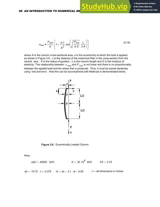
3.12.1 Maximum Design Load for a Column
A steel pipe with an outside diameter of 10.70 inches and a wall thickness of 0.375 inches is
to serve as a pin-ended column that is 22 feet long . It supports an eccentric load at an
eccentricity of e = 1.5 inches from the column center-line. The maximum load that the
column can carry with a factor of safety of 2.75 is to be determined. The modulus of
elasticity E for steel is 30 x 10 6 psi and its yield strength, σyld , is 40,000 psi .
The equation for the stress level σ max resulting from the application of the maximum load
P max is [ 3,18 ]
Chapter 3: Roots of Equations 87](https://image.slidesharecdn.com/anintroductiontonumericalmethodsusingmathcadmathcadrelease14-230805170449-0ea94cc2/85/AN-INTRODUCTION-TO-NUMERICAL-METHODS-USING-MATHCAD-Mathcad-Release-14-97-320.jpg)
![e 1.50
:= L 264.
:= c
do
2
:= c 5.35
=
I
π
64
do
4
di
4
−
( )
⋅
:= ( in 4 ) A
π
4
do
2
di
2
−
( )
⋅
:= (in 2 )
A 12.1639
= I 162.3057
= K
I
A
:= K 3.6528
= (in )
With a factor of safety of 2.75, the maximum stress level that the column can have is
σmax
σyld
FS
:= σmax 1.4545 10
4
×
= psi
The corresponding maximum allowable load may be determined from Equation (3.18) using
the root function as follows.
g Pmax
( )
Pmax
E A
⋅
L
2 K
⋅
⋅
:=
f Pmax
( ) σmax
Pmax
A
1
e c
⋅
K
2
sec g Pmax
( )
( )
⋅
+
⎛
⎜
⎝
⎞
⎟
⎠
⋅
−
:=
Pmax 125000.
:= (lbs) <--Guess value for the root
a root f Pmax
( ) Pmax
,
( )
:=
a 1.0221 10
5
×
= (lbs) <-- Maximum allowable load column can carry
3.12.2. Natural Frequencies of Vibration of a Uniform Beam
For a uniform beam that is clamped at one end and free at the other, a shown in Figure 3.7 ,
the natural frequencies of vibration [20] are given by the equation
1 cos βprime
( ) cosh βprime
( )
⋅
+ 0
= (3.19)
Chapter 3: Roots of Equations 89](https://image.slidesharecdn.com/anintroductiontonumericalmethodsusingmathcadmathcadrelease14-230805170449-0ea94cc2/85/AN-INTRODUCTION-TO-NUMERICAL-METHODS-USING-MATHCAD-Mathcad-Release-14-99-320.jpg)
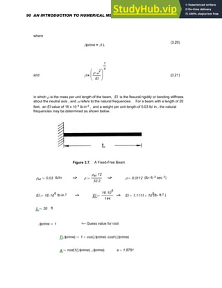
![β
a
L
:= β 0.0938
=
ω
EI β
4
⋅
ρ
:= ω 27.7106
= (rad/sec) <-- First or fundamental
natural frequency
βprime 5
:= <-- Guess value for next root
f βprime
( ) 1 cos βprime
( ) cosh βprime
( )
⋅
+
:=
a root f βprime
( ) βprime
,
( )
:=
a 4.6941
=
β
a
L
:= β 0.2347
=
ω
EI β
4
⋅
ρ
:= ω 173.6595
= (rad/sec) <-- Second natural frequency
Similarly by making appropriate guesses, higher natural frequencies can be determined
using the root function. Some of these are listed below.
Third natural frequency: 486.3 rad/sec
Fourth natural frequency: 952.8 rad/sec
Fifth natural frequency: 1575.1 rad/sec
Sixth natural frequency: 2353 rad/sec
Seventh natural frequency: 3286 rad/sec.
3.12.3. Solving the Characteristic Equation in Control Systems Engineering
A characteristic equation is an algebraic equation that is formulated from the differential
equation or equations of a control system [14] . Its solution, which often requires evaluation
of the roots of a polynomial of degree higher than two, is crucial in determining system
stability and assessing system transient response in terms of its time constant, natural
frequencies , damping qualities etc. An application involving the use of Mathcad' s polyroots
function in determining the roots of a characteristic polynomial of a control system is
presented below.
Chapter 3: Roots of Equations 91](https://image.slidesharecdn.com/anintroductiontonumericalmethodsusingmathcadmathcadrelease14-230805170449-0ea94cc2/85/AN-INTRODUCTION-TO-NUMERICAL-METHODS-USING-MATHCAD-Mathcad-Release-14-101-320.jpg)
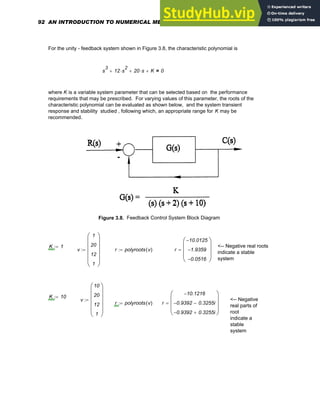
![<-- Negative
real parts
of root
indicate a
stable
system
K 100
:= v
100
20
12
1
⎛
⎜
⎜
⎜
⎜
⎝
⎞
⎟
⎟
⎟
⎟
⎠
:= r polyroots v
( )
:= r
11.0084
−
0.4958
− 2.9729i
+
0.4958
− 2.9729i
−
⎛
⎜
⎜
⎜
⎝
⎞
⎟
⎟
⎟
⎠
=
<-- Positive
real
parts of root
indicate an
unstable
system
K 400
:= v
400
20
12
1
⎛
⎜
⎜
⎜
⎜
⎝
⎞
⎟
⎟
⎟
⎟
⎠
:= r polyroots v
( )
:= r
12.8628
−
0.4314 5.5598i
+
0.4314 5.5598i
−
⎛
⎜
⎜
⎜
⎝
⎞
⎟
⎟
⎟
⎠
=
3.12.4. Horizontal Tension in a Uniform Cable
Flexible cables are often used in suspension bridges, transmission lines, telephone lines ,
mooring lines and many other applications. A cable hanging under its own weight takes the
shape of a catenary in which the deflection y along the span is given by the following
relationship [ 8 ]
y
H
w
cosh
w x
⋅
H
⎛
⎜
⎝
⎞
⎟
⎠
1
−
⎛
⎜
⎝
⎞
⎟
⎠
⋅
= (3.22)
where x is the horizontal distance along the span a shown in Figure 3.9 , H is the horizontal
component of tension in the cable and w is the weight per unit length of the cable.
Figure 3.9. Catenary cable
Chapter 3: Roots of Equations 93](https://image.slidesharecdn.com/anintroductiontonumericalmethodsusingmathcadmathcadrelease14-230805170449-0ea94cc2/85/AN-INTRODUCTION-TO-NUMERICAL-METHODS-USING-MATHCAD-Mathcad-Release-14-103-320.jpg)


![3.24. The dynamic response of an underdamped second-order system, which is a
common mathematical model in control system analysis, to a unit step function is given
by [ 14 ]
c t
( ) 1
1
1 ζ
2
−
e
ζ
− ωn
⋅ t
⋅
⋅ cos ωn 1 ζ
2
−
⋅ t
⋅ ϕ
−
⎛
⎝
⎞
⎠
⎡
⎣
⎤
⎦
⋅
−
=
where ζ is the system damping ratio, ω n is the undamped natural frequency, and φ is
ϕ atan
ζ
1 ζ
2
−
⎛
⎜
⎜
⎝
⎞
⎟
⎟
⎠
=
A precise analytical relationship between the damping ratio and the rise time which is the time
required for the response to go from 10 % of the final value to 90 % ( that is, from 0.1 to 0.9 in
this case ) cannot be determined . However, using Mathcad's root function, the normalized
rise time which is ω n times the rise time, can be found for a specified damping ratio ζ by
solving for the values of ω n t that yield c(t) = 0.9 and c(t)= 0.1 . Subtracting these two values
yields the normalized rise time for the value of ζ considered . Using a range of damping ratios
from 0.1, 0.2, 0.3... .. 0.9 , construct a plot depicting normalized rise time as a function of
the damping ratio .
3.25. The frequency equation for the free undamped longitudinal vibration of a slender bar
of length L and mass m with one end fixed and with the other end carrying a mass M is
given by [ 21 ]
β tan β
( )
⋅ α
=
where
β ω
L
c0
⋅
=
c0
E
ρ
=
Figure P 3.25.
100 AN INTRODUCTION TO NUMERICAL METHODS USING MATHCAD](https://image.slidesharecdn.com/anintroductiontonumericalmethodsusingmathcadmathcadrelease14-230805170449-0ea94cc2/85/AN-INTRODUCTION-TO-NUMERICAL-METHODS-USING-MATHCAD-Mathcad-Release-14-110-320.jpg)
![α
m
M
=
in which E is Young's modulus for the material of the bar, ρ is the mass per unit volume and
ω is the natural frequency .
For a steel bar with mass ratio α = 0.70, E = 30 x 10 6 psi , L = 98 in., and ρ = 7.35x 10 -4
lb-sec 2 / in 4 , determine the first three natural frequencies.
3.26. For a uniform beam of length L with one end fixed and the other simply supported, the
natural frequencies of transverse vibration are given by the relationship [ 21 ]
tan k L
⋅
( ) tanh k L
⋅
( )
=
where
k
2
ω
ρ A
⋅
E I
⋅
⋅
=
Figure P 3.26
in which ω is the natural frequency , ρ is the mass density of the beam material, A is the
area of cross section of the beam , E is Young's modulus, and I is the moment of inertia of
the beam cross section.
Determine the first three natural frequencies of a 36 in. long steel beam whose area of
cross section A is 12.50 in 2 , moment of inertia I is 12.75 in 4, and ρ = 7.35x 10 -4 lb-sec 2 /
in 4 . E for steel is 30 x 10 6 psi.
Chapter 3: Roots of Equations 101](https://image.slidesharecdn.com/anintroductiontonumericalmethodsusingmathcadmathcadrelease14-230805170449-0ea94cc2/85/AN-INTRODUCTION-TO-NUMERICAL-METHODS-USING-MATHCAD-Mathcad-Release-14-111-320.jpg)

![For the above case, C12 1
−
( )
3
31
( )
⋅
:= , that is, C12 31
−
=
Adjoint Matrix:
The adjoint of a square matrix is the transpose of the matrix of its cofactors.
Inverse of a Matrix:
The inverse A -1 of a matrix A must satisfy the relationship
A A -1 = I , (4.3)
where I is the Identity or the Unit matrix which is a matrix with "1" along the diagonal and
zero elsewhere. The inverse A -1 is calculated as follows
A -1 = [adjoint (A)] / Det (A) , (4.4)
where Det (A) is the determinant of the given matrix, which must be non-zero for the inverse to
exist.
Example 4.1
Determine the inverse of the following matrix A
A
1
1
1
2
3
0
3
2
4
⎛
⎜
⎜
⎜
⎝
⎞
⎟
⎟
⎟
⎠
:=
The determinant of this matrix is A 1
−
=
The minors of A are
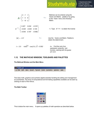
M11
3
0
2
4
⎛
⎜
⎝
⎞
⎟
⎠
:= M12
1
1
2
4
⎛
⎜
⎝
⎞
⎟
⎠
:= M13
1
1
3
0
⎛
⎜
⎝
⎞
⎟
⎠
:=
M21
2
0
3
4
⎛
⎜
⎝
⎞
⎟
⎠
:= M22
1
1
3
4
⎛
⎜
⎝
⎞
⎟
⎠
:= M23
1
1
2
0
⎛
⎜
⎝
⎞
⎟
⎠
:=
104 AN INTRODUCTION TO NUMERICAL METHODS USING MATHCAD](https://image.slidesharecdn.com/anintroductiontonumericalmethodsusingmathcadmathcadrelease14-230805170449-0ea94cc2/85/AN-INTRODUCTION-TO-NUMERICAL-METHODS-USING-MATHCAD-Mathcad-Release-14-114-320.jpg)

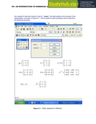
![Given the two matrices A and B:
A
1
1
7
0
3
8
2
2
9
⎛
⎜
⎜
⎜
⎝
⎞
⎟
⎟
⎟
⎠
:= B
3
1
1
2
2
5
1
3
9
⎛
⎜
⎜
⎜
⎝
⎞
⎟
⎟
⎟
⎠
:=
Addition:
A B
+
4
2
8
2
5
13
3
5
18
⎛
⎜
⎜
⎜
⎝
⎞
⎟
⎟
⎟
⎠
=
Subtraction:
A B
−
2
−
0
6
2
−
1
3
1
1
−
0
⎛
⎜
⎜
⎜
⎝
⎞
⎟
⎟
⎟
⎠
=
Multiplication:
<--Use the asterisk ( * ) to multiply two matrices
A B
⋅
5
8
38
12
18
75
19
28
112
⎛
⎜
⎜
⎜
⎝
⎞
⎟
⎟
⎟
⎠
=
<-- Order in which multiplication is done is important.
Note that [A] [B] is not equal to [B][A]
B A
⋅
12
24
69
14
30
87
19
33
93
⎛
⎜
⎜
⎜
⎝
⎞
⎟
⎟
⎟
⎠
=
Scalar subtraction:
A 5
−
4
−
4
−
2
5
−
2
−
3
3
−
3
−
4
⎛
⎜
⎜
⎜
⎝
⎞
⎟
⎟
⎟
⎠
=
Chapter 4: Matrices and Linear Algebra 107](https://image.slidesharecdn.com/anintroductiontonumericalmethodsusingmathcadmathcadrelease14-230805170449-0ea94cc2/85/AN-INTRODUCTION-TO-NUMERICAL-METHODS-USING-MATHCAD-Mathcad-Release-14-117-320.jpg)
![Scalar multiplication: ( Use the asterisk "*" )
A 5
⋅
5
5
35
0
15
40
10
10
45
⎛
⎜
⎜
⎜
⎝
⎞
⎟
⎟
⎟
⎠
=
Matrix inverse: Use : ^ -1
A
1
−
0.733
−
0.333
−
0.867
1.067
−
0.333
0.533
0.4
0
0.2
−
⎛
⎜
⎜
⎜
⎝
⎞
⎟
⎟
⎟
⎠
=
Determinant of A : A 15
−
=
Transpose of A: Use [Ctrl]1
A
T
1
0
2
1
3
2
7
8
9
⎛
⎜
⎜
⎜
⎝
⎞
⎟
⎟
⎟
⎠
=
Matrix subscripts:
Use " [ " to put in subscripts. Note that, in this case, subscripts will go from 0 to 2.
because, in Mathcad, vector and matrix elements are ordinarily numbered starting with row
zero and column zero. To make " one " the " ORIGIN " , go to the Tools menu, choose
Worksheet Options , as shown in Figure 4.2 , and change the array origin from 0 to 1.
4.3 SOLUTION OF LINEAR ALGEBRAIC EQUATIONS BY USING
THE INVERSE
For a system of linear algebraic equations that can be written in matrix form as
[A]{X} = {B} (4.5)
where the matrix [A] and the column vector {B} contain known constants, the inverse of the matrix
[A] can be utilized in the determination of the solution vector {X} as follows
{X} = [A] -1 {B} (4.6)
108 AN INTRODUCTION TO NUMERICAL METHODS USING MATHCAD](https://image.slidesharecdn.com/anintroductiontonumericalmethodsusingmathcadmathcadrelease14-230805170449-0ea94cc2/85/AN-INTRODUCTION-TO-NUMERICAL-METHODS-USING-MATHCAD-Mathcad-Release-14-118-320.jpg)
![Example 4.2
Solve: 2x + 4 y + z = -11
-x + 3 y -2 z = -16
2x - 3y + 5 z = 21
Putting the given equations in the form [A] {X}= {B}, where
A
2
1
−
2
4
3
3
−
1
2
−
5
⎛
⎜
⎜
⎜
⎝
⎞
⎟
⎟
⎟
⎠
:= B
11
−
16
−
21
⎛
⎜
⎜
⎜
⎝
⎞
⎟
⎟
⎟
⎠
:=
The inverse of [A] can be easily obtained as
A
1
−
0.474
0.053
0.158
−
1.211
−
0.421
0.737
0.579
−
0.158
0.526
⎛
⎜
⎜
⎜
⎝
⎞
⎟
⎟
⎟
⎠
=
and [A] multiplied by [A]-1 will yield the identity matrix as shown
A A
1
−
⋅
1
0
0
0
1
0
0
0
1
⎛
⎜
⎜
⎜
⎝
⎞
⎟
⎟
⎟
⎠
=
The solution can then be generated by performing the matrix operation
X A
1
−
B
⋅
:=
yielding
X
2
4
−
1
⎛
⎜
⎜
⎜
⎝
⎞
⎟
⎟
⎟
⎠
=
4.4 SOLUTION OF LINEAR ALGEBRAIC EQUATIONS BY
CRAMER'S RULE
As an alternative to the above procedure, the solution {X} to the matrix equation
(Equation 4.5)
110 AN INTRODUCTION TO NUMERICAL METHODS USING MATHCAD](https://image.slidesharecdn.com/anintroductiontonumericalmethodsusingmathcadmathcadrelease14-230805170449-0ea94cc2/85/AN-INTRODUCTION-TO-NUMERICAL-METHODS-USING-MATHCAD-Mathcad-Release-14-120-320.jpg)
![[A] {X} = {B}
can be computed using Cramer's rule as shown below
Letting
A
A11
A21
A31
A12
A22
A32
A13
A23
A33
⎛
⎜
⎜
⎜
⎝
⎞
⎟
⎟
⎟
⎠
= B
B1
B2
B3
⎛
⎜
⎜
⎜
⎝
⎞
⎟
⎟
⎟
⎠
=
the solution {X} can be computed using
X1
B1
B2
B3
A12
A22
A32
A13
A23
A33
⎛
⎜
⎜
⎜
⎝
⎞
⎟
⎟
⎟
⎠
A11
A21
A31
A12
A22
A32
A13
A23
A33
⎛
⎜
⎜
⎜
⎝
⎞
⎟
⎟
⎟
⎠
= X2
A11
A21
A31
B1
B2
B3
A13
A23
A33
⎛
⎜
⎜
⎜
⎝
⎞
⎟
⎟
⎟
⎠
A11
A21
A31
A12
A22
A32
A13
A23
A33
⎛
⎜
⎜
⎜
⎝
⎞
⎟
⎟
⎟
⎠
=
(4.7)
X3
A11
A21
A31
A12
A22
A32
B1
B2
B3
⎛
⎜
⎜
⎜
⎝
⎞
⎟
⎟
⎟
⎠
A11
A21
A31
A12
A22
A32
A13
A23
A33
⎛
⎜
⎜
⎜
⎝
⎞
⎟
⎟
⎟
⎠
=
For Example 4.2,
A
2
1
−
2
4
3
3
−
1
2
−
5
⎛
⎜
⎜
⎜
⎝
⎞
⎟
⎟
⎟
⎠
:= B
11
−
16
−
21
⎛
⎜
⎜
⎜
⎝
⎞
⎟
⎟
⎟
⎠
:= D A
:= D 19
=
Chapter 4: Matrices and Linear Algebra 111](https://image.slidesharecdn.com/anintroductiontonumericalmethodsusingmathcadmathcadrelease14-230805170449-0ea94cc2/85/AN-INTRODUCTION-TO-NUMERICAL-METHODS-USING-MATHCAD-Mathcad-Release-14-121-320.jpg)
![,
x
B1
B2
B3
A1 2
,
A2 2
,
A3 2
,
A1 3
,
A2 3
,
A3 3
,
⎛
⎜
⎜
⎜
⎝
⎞
⎟
⎟
⎟
⎠
D
:= y
A1 1
,
A2 1
,
A3 1
,
B1
B2
B3
A1 3
,
A2 3
,
A3 3
,
⎛
⎜
⎜
⎜
⎝
⎞
⎟
⎟
⎟
⎠
D
:= z
A1 1
,
A2 1
,
A3 1
,
A1 2
,
A2 2
,
A3 2
,
B1
B2
B3
⎛
⎜
⎜
⎜
⎝
⎞
⎟
⎟
⎟
⎠
D
:=
where the matrix elements have been specified in the format required by Mathcad. These
calculations result in
x 2
= y 4
−
= z 1
=
4.5 SOLUTION OF LINEAR ALGEBRAIC EQUATIONS USING THE
FUNCTION lsolve
The lsolve function in Mathcad can be used to solve a system of linear algebraic equations .
Given:
[A] {X}= {B},
the function lsolve (A,B) will return the solution vector {X}, provided the matrix [A] is not
singular or nearly singular. For Example 4.2,
A
2
1
−
2
4
3
3
−
1
2
−
5
⎛
⎜
⎜
⎜
⎝
⎞
⎟
⎟
⎟
⎠
= B
11
−
16
−
21
⎛
⎜
⎜
⎜
⎝
⎞
⎟
⎟
⎟
⎠
=
X lsolve A B
,
( )
:= gives X
2
4
−
1
⎛
⎜
⎜
⎜
⎝
⎞
⎟
⎟
⎟
⎠
=
Example 4.3
Application of Matrices to Electrical Circuit Analysis.
Formulate a set of linear equations that represent the relationship between voltage, current and
resistances for the circuit shown in Figure 4.3. Solve the simultaneous equations generated using
(1) the inverse (2) Cramer's Rule and (3) the Mathcad function lsolve
112 AN INTRODUCTION TO NUMERICAL METHODS USING MATHCAD](https://image.slidesharecdn.com/anintroductiontonumericalmethodsusingmathcadmathcadrelease14-230805170449-0ea94cc2/85/AN-INTRODUCTION-TO-NUMERICAL-METHODS-USING-MATHCAD-Mathcad-Release-14-122-320.jpg)
![Figure 4.3. Electrical circuit example
The governing equations are:
i1 + i2 = i3
7 i1 + 3 i3 = 6
7 i1 - 5 i2 = 6
These must be put in the form: [A] {X} = {B} and solved for {X}
Using the inverse
A
1
7
7
1
0
5
−
1
−
3
0
⎛
⎜
⎜
⎜
⎝
⎞
⎟
⎟
⎟
⎠
:= B
0
6
6
⎛
⎜
⎜
⎜
⎝
⎞
⎟
⎟
⎟
⎠
:=
<--These are the currents i1, i2 and
i3
X A
1
−
B
⋅
:= X
0.6761
0.2535
−
0.4225
⎛
⎜
⎜
⎜
⎝
⎞
⎟
⎟
⎟
⎠
=
Using Cramer's Rule
L
0
6
6
1
0
5
−
1
−
3
0
⎛
⎜
⎜
⎜
⎝
⎞
⎟
⎟
⎟
⎠
:= M
1
7
7
0
6
6
1
−
3
0
⎛
⎜
⎜
⎜
⎝
⎞
⎟
⎟
⎟
⎠
:= N
1
7
7
1
0
5
−
0
6
6
⎛
⎜
⎜
⎜
⎝
⎞
⎟
⎟
⎟
⎠
:=
i1
L
A
:= i2
M
A
:= i3
N
A
:= i1 0.676
= i2 0.254
−
= i3 0.4225
=
Chapter 4: Matrices and Linear Algebra 113](https://image.slidesharecdn.com/anintroductiontonumericalmethodsusingmathcadmathcadrelease14-230805170449-0ea94cc2/85/AN-INTRODUCTION-TO-NUMERICAL-METHODS-USING-MATHCAD-Mathcad-Release-14-123-320.jpg)
![Using Mathcad Function lsolve
X lsolve A B
,
( )
:= X
0.676
0.254
−
0.423
⎛
⎜
⎜
⎜
⎝
⎞
⎟
⎟
⎟
⎠
= <--These are the currents i1, i2 and i3
4.6 THE EIGENVALUE PROBLEM
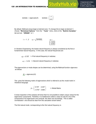
Eigenvalue problems occur in a variety of physical situations. Some examples of eigenvalue
problems are given below.
1. Determination of natural frequencies and mode shapes of oscillating systems.
2. Computation of principal stresses and principal directions
3. Computation of principal moments of inertia and principal axes.
4. Buckling of structures.
5. Oscillations of electrical networks.
The eigenvalue problem can be mathematically stated as
[A] {X} = λ {X} (4.8)
where [A] is a known square matrix, {X} is a column vector of unknowns, and λ is an unknown
scalar quantity. The solution of the eigenvalue problem involves the determination of vectors
{X} and associated constants λ satisfying equation (4.8). These vectors {X} are termed
eigenvectors. With each eigenvector is associated a constant λ which is called an
eigenvalue.
Equation (4.8) can be written in the form
[A- λ I ] {X} = {0} (4.9)
A trivial solution to the above is
{X} = 0
which is not of interest to us. The condition for the existence of a non-trivial solution is
det ( A- λ I ) = 0 (4.10)
114 AN INTRODUCTION TO NUMERICAL METHODS USING MATHCAD](https://image.slidesharecdn.com/anintroductiontonumericalmethodsusingmathcadmathcadrelease14-230805170449-0ea94cc2/85/AN-INTRODUCTION-TO-NUMERICAL-METHODS-USING-MATHCAD-Mathcad-Release-14-124-320.jpg)
![Expansion of the above determinant produces a polynomial in λ. For instance, if [A] is a 3x 3
matrix, then Equation (4.10) would give a cubic in λ. This polynomial is called the
characteristic polynomial and its roots are called eigenvalues. Associated with each
eigenvalue is a solution vector {X} called the eigenvector.
It can be shown that the adjoint of matrix (A- λiI) contains columns, each of which is the ith
eigenvector {X} i associated with the eigenvalue λ i multiplied by an arbitrary constant.
Thus, to determine an eigenvector corresponding to an eigenvalue λi , compute the adjoint of
(A- λiI) and choose any column of it as the eigenvector.
Example 4.4
Compute the eigenvalues and eigenvectors of
17
45
6
−
16
−
⎛
⎜
⎝
⎞
⎟
⎠
A
17
45
6
−
16
−
⎛
⎜
⎝
⎞
⎟
⎠
:=
The [A- λI] matrix can be written as
A λ I
⋅
−
17 λ
−
45
6
−
16
− λ
−
⎛
⎜
⎝
⎞
⎟
⎠
=
A non-trivial solution is obtained by setting the determinant of [ A - λ I ] equal to zero
17 λ
−
45
6
−
16
− λ
−
⎛
⎜
⎝
⎞
⎟
⎠
0
=
which gives λ 2 - λ - 2 = 0, or, λ 1 = 2, λ 2 = -1. The adjoint of the matrix (A- λ I ), in
this case, is
16
− λ
−
45
−
6
17 λ
−
⎛
⎜
⎝
⎞
⎟
⎠
For λ 1 = 2, the corresponding eigenvector is the first or second column of the above
adjoint matrix with λ = λ 1 which gives
Chapter 4: Matrices and Linear Algebra 115](https://image.slidesharecdn.com/anintroductiontonumericalmethodsusingmathcadmathcadrelease14-230805170449-0ea94cc2/85/AN-INTRODUCTION-TO-NUMERICAL-METHODS-USING-MATHCAD-Mathcad-Release-14-125-320.jpg)

![differential equations of motion can be seen to be
2 m d2x1 /dt2 + 3 k x1 - k x2 = 0
m d2x2 /dt2 +k ( x2 - x1 ) = 0
(4.11)
Expressing the above equations in matrix form as
..
(4.12)
[M] {x} + [K ] {x} = {0}
where [M] is the mass or inertia matrix , and [K] is the stiffness matrix, and assuming that
{x} = {A}sin ωt (4.13)
we obtain a set of linear homogeneous algebraic equations that can be written in matrix form as
(4.14)
([K]- ω2 [M ] ) {A} = 0
For a non-trivial solution, the determinant | K- ω2 M | must be zero. The problem can also be
posed slightly differently in the familiar form
|A-λI| = 0 (4.15)
where the λ 's ( λ = ω2) are the eigenvalues of the matrix [A] , which, in this case, is
[A] = [M] -1 [K] (4.16)
To find the natural frequencies and mode shapes in this case, we need to determine the
eigenvalues and eigenvectors of the matrix [A]. The square roots of the eigenvalues will then
give the natural frequencies and the corresponding eigenvectors will be the mode shapes.
Letting m = 1, and k =1 in this problem for convenience
m 1
:= k 1
:=
Then, the mass and stiffness matrices
M
2 m
⋅
0
0
m
⎛
⎜
⎝
⎞
⎟
⎠
:= K
3 k
⋅
k
−
k
−
k
⎛
⎜
⎝
⎞
⎟
⎠
:=
118 AN INTRODUCTION TO NUMERICAL METHODS USING MATHCAD](https://image.slidesharecdn.com/anintroductiontonumericalmethodsusingmathcadmathcadrelease14-230805170449-0ea94cc2/85/AN-INTRODUCTION-TO-NUMERICAL-METHODS-USING-MATHCAD-Mathcad-Release-14-128-320.jpg)
![give
M
2
0
0
1
⎛
⎜
⎝
⎞
⎟
⎠
= K
3
1
−
1
−
1
⎛
⎜
⎝
⎞
⎟
⎠
=
The [A] matrix, which is called the dynamic matrix in the language of vibrations is ,
A M
1
−
K
⋅
:= which gives A
1.5
1
−
0.5
−
1
⎛
⎜
⎝
⎞
⎟
⎠
=
The eigenvalues of [A] are obtained from setting the determinant of [A-λI] equal to zero, as
follows
A λ I
⋅
− 0
=
This yields
1.5 λ
−
( ) 1 λ
−
( )
⋅ 0.5
− 0
= , or, λ1 = 0.5 , and λ2 = 2
The adjoint of the matrix [A-λI] is
1 λ
−
( )
1
0.5
1.5 λ
−
( )
⎡
⎢
⎣
⎤
⎥
⎦
In Vibration Engineering, eigenvectors are termed as natural modes or mode shapes, and
these are simply the configurations that the system takes when vibrating at a natural
frequency. Because the system considered here is a two-degree-of-freedom system, there
will be two natural frequencies and correspondingly two modes. While the natural
frequencies are simply the square roots of the eigenvalues, the associated eigenvectors or
modeshapes can be determined by putting λ = λ1(for the first mode ) and λ = λ2 (for the
second mode ) in either column of the adjoint of [A- λ I]
This procedure generates the following mode shapes
FirstMode
0.5
1
⎛
⎜
⎝
⎞
⎟
⎠
:= and SecondMode
1
1
⎛
⎜
⎝
⎞
⎟
⎠
:=
The determination of eigenvalues and eigenvectors using Mathcad is done below.
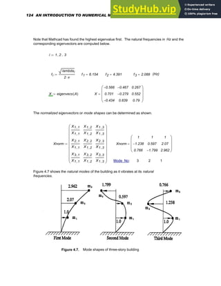
Chapter 4: Matrices and Linear Algebra 119](https://image.slidesharecdn.com/anintroductiontonumericalmethodsusingmathcadmathcadrelease14-230805170449-0ea94cc2/85/AN-INTRODUCTION-TO-NUMERICAL-METHODS-USING-MATHCAD-Mathcad-Release-14-129-320.jpg)
![Figure 4.6. Mathematical model of three-story building
The equations of motion of the mathematical model resorted to can be shown to be
m1
2
t
x1
d
d
2
⋅ k1 x1
⋅
+ k2 x2 x1
−
( )
⋅
− 0
=
m2
2
t
x2
d
d
2
⋅ k2 x2 x1
−
( )
⋅
+ k3 x3 x2
−
( )
⋅
− 0
= (4.17)
m3
2
t
x3
d
d
2
⋅ k3 x3 x2
−
( )
⋅
+ 0
=
These can be put in the following matrix format
[M] d2 {x} /dt2 + {K] { x } = { 0} (4.18)
where
122 AN INTRODUCTION TO NUMERICAL METHODS USING MATHCAD](https://image.slidesharecdn.com/anintroductiontonumericalmethodsusingmathcadmathcadrelease14-230805170449-0ea94cc2/85/AN-INTRODUCTION-TO-NUMERICAL-METHODS-USING-MATHCAD-Mathcad-Release-14-132-320.jpg)
![[M] =
m1
0
0
0
m2
0
0
0
m3
⎛
⎜
⎜
⎜
⎝
⎞
⎟
⎟
⎟
⎠
(4.19)
[K] =
k1 k2
+
( )
k2
−
0
k2
−
k2 k3
+
( )
k3
−
0
k3
−
k3
⎡
⎢
⎢
⎢
⎣
⎤
⎥
⎥
⎥
⎦
Letting m1 = 2x 10 6 kg , m2 = 14x 10 5 kg , m3 = 7x10 5 kg; and k1 = 12x10 8 N/ m,
k2= 8x 10 8 N/m , k3 = 4x 10 8 N/ m , the [A] matrix can be computed, using Mathcad ,
as follows
m1 2 10
6
⋅
:= m2 14 10
5
⋅
:= m3 7 10
5
⋅
:= k1 12 10
8
⋅
:= k2 8 10
8
⋅
:= k3 4 10
8
⋅
:=
M
m1
0
0
0
m2
0
0
0
m3
⎛
⎜
⎜
⎜
⎝
⎞
⎟
⎟
⎟
⎠
:= K
k1 k2
+
( )
k2
−
0
k2
−
k2 k3
+
( )
k3
−
0
k3
−
k3
⎡
⎢
⎢
⎢
⎣
⎤
⎥
⎥
⎥
⎦
:=
M
2 10
6
⋅
0
0
0
1.4 10
6
⋅
0
0
0
0.7 10
6
⋅
⎛
⎜
⎜
⎜
⎜
⎝
⎞
⎟
⎟
⎟
⎟
⎠
:= K
2 10
9
×
8
− 10
8
×
0
8
− 10
8
×
1.2 10
9
×
4
− 10
8
×
0
4
− 10
8
×
4 10
8
×
⎛
⎜
⎜
⎜
⎜
⎝
⎞
⎟
⎟
⎟
⎟
⎠
=
A M
1
−
K
⋅
:= A
1 10
3
×
571.429
−
0
400
−
857.143
571.429
−
0
285.714
−
571.429
⎛
⎜
⎜
⎜
⎝
⎞
⎟
⎟
⎟
⎠
=
The eigenvalues and the eigenvectors are
lambda eigenvals A
( )
:= lambda
1.495 10
3
×
761.106
172.146
⎛
⎜
⎜
⎜
⎝
⎞
⎟
⎟
⎟
⎠
=
Chapter 4: Matrices and Linear Algebra 123](https://image.slidesharecdn.com/anintroductiontonumericalmethodsusingmathcadmathcadrelease14-230805170449-0ea94cc2/85/AN-INTRODUCTION-TO-NUMERICAL-METHODS-USING-MATHCAD-Mathcad-Release-14-133-320.jpg)
![4.9 APPLICATION OF THE EIGENVALUE PROBLEM TO STRESS
ANALYSIS- DETERMINATION OF PRINCIPAL STRESSES AND
PRINCIPAL DIRECTIONS
If [σ ] is the state of stress at a point in a material given by the stress components σxx ,
σyy, σzz, σxy , σyz and σzx , the principal stresses are the eigenvalues λ of the stress matrix
and the principal directions, which are the x, y and z components of the unit vectors along
the normals to the principal planes , are the eigenvectors {η} of the stress matrix. Thus ,
the eigenvalue problem in this case is stated as
[σ] - λ [ I ]) { η } = {0} (4.20)
where the eigenvalues λ and the eigenvectors η are to be determined.
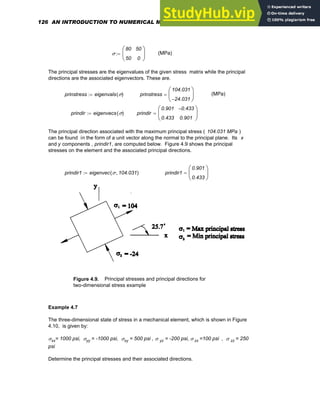
Example 4.6
The two-dimensional state of stress in a mechanical element, which is shown in Figure 4.8, is
given by the components:
σ xx = 80 MPa, σyy = 0 , and σ xy = 50 MPa.
Determine the principal stresses and their associated directions.
Figure 4.8. Two-dimensional state of stress
Because the stress matrix is symmetrical, σ yx must be equal to σ xy. Thus, the matrix of
stresses is
Chapter 4: Matrices and Linear Algebra 125](https://image.slidesharecdn.com/anintroductiontonumericalmethodsusingmathcadmathcadrelease14-230805170449-0ea94cc2/85/AN-INTRODUCTION-TO-NUMERICAL-METHODS-USING-MATHCAD-Mathcad-Release-14-135-320.jpg)
![considered as eigenvectors. The following examples will illustrate this situation.
Example 4.8
For the given matrix [A]
A
0
1
−
1
1
−
0
1
1
1
0
⎛
⎜
⎜
⎜
⎝
⎞
⎟
⎟
⎟
⎠
:=
the eigenvalues and eigenvectors are found using Mathcad as
<-- double root at λ = 1
lambda eigenvals A
( )
:= lambda
1
2
−
1
⎛
⎜
⎜
⎜
⎝
⎞
⎟
⎟
⎟
⎠
=
X eigenvecs A
( )
:= X
0.816
0.408
−
0.408
0.577
−
0.577
−
0.577
0.226
−
0.793
0.566
⎛
⎜
⎜
⎜
⎝
⎞
⎟
⎟
⎟
⎠
=
It is clear that the first and third eigenvectors corresponding to the repeated root λ = 1 are
arbitrary, since they are both different , while the one corresponding to λ = - 2 is
1
−
1
−
1
⎛
⎜
⎜
⎜
⎝
⎞
⎟
⎟
⎟
⎠
Example 4.9
The following problem is, clearly, a case of repeated roots with a double root at λ = 1
Chapter 4: Matrices and Linear Algebra 129](https://image.slidesharecdn.com/anintroductiontonumericalmethodsusingmathcadmathcadrelease14-230805170449-0ea94cc2/85/AN-INTRODUCTION-TO-NUMERICAL-METHODS-USING-MATHCAD-Mathcad-Release-14-139-320.jpg)
![A
1
0
0
1
−
1
0
0
1
1
−
⎛
⎜
⎜
⎜
⎝
⎞
⎟
⎟
⎟
⎠
:=
The eigenvalues and eigenvectors are
lambda eigenvals A
( )
:= lambda
1
1
1
−
⎛
⎜
⎜
⎜
⎝
⎞
⎟
⎟
⎟
⎠
=
X eigenvecs A
( )
:= X
1
0
0
1
0
0
0.218
−
0.436
−
0.873
⎛
⎜
⎜
⎜
⎝
⎞
⎟
⎟
⎟
⎠
=
Note that the first and second eigenvectors corresponding to the repeated (double) root at λ
= 1 are, in fact , arbitrary since they have two components that are zero, while the one
corresponding to λ = -1 is the third one which is
1
−
2
−
4
⎛
⎜
⎜
⎜
⎝
⎞
⎟
⎟
⎟
⎠
Example 4.10
For the following matrix [A]
A
14
−
0
1
1
2
0
0
0
2
⎛
⎜
⎜
⎜
⎝
⎞
⎟
⎟
⎟
⎠
:=
the eigenvalues and eigenvectors are
130 AN INTRODUCTION TO NUMERICAL METHODS USING MATHCAD](https://image.slidesharecdn.com/anintroductiontonumericalmethodsusingmathcadmathcadrelease14-230805170449-0ea94cc2/85/AN-INTRODUCTION-TO-NUMERICAL-METHODS-USING-MATHCAD-Mathcad-Release-14-140-320.jpg)
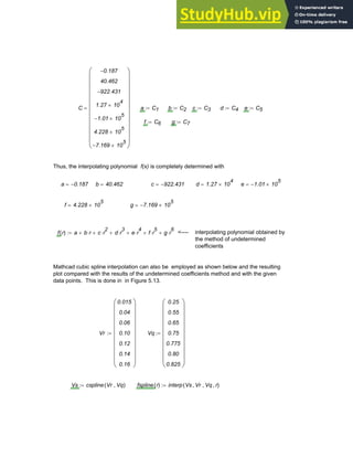
![ah + bj = -p and ch + d j = -q (4.24)
When these two simultaneous equations are solved for h and j , we generate new
improved values for x and y, say x i+1 and y i+1 , where , x i + 1 = x i + h and y i+1 = yi +
j . These new improved values replace the old values x i and y i in the next step in an effort
to obtain still better solutions. This procedure is repeated until convergence occurs. The
following example will clarify the procedure.
Example 4.11
Determine the solution to: f(x,y) = x2 + 3 y 2 - 54 = 0 , g(x, y ) = -4 x 2 + 3x y - 2 y + 15 = 0
Iteration Number 1
f x y
,
( ) x
2
3 y
2
⋅
+ 54
−
:= g x y
,
( ) 4
− x
2
⋅ 3 x
⋅ y
⋅
+ 2 y
⋅
− 15
+
:=
partfx x y
,
( ) 2 x
⋅
:= partfy x y
,
( ) 6 y
⋅
:= partgx x y
,
( ) 8
− x
⋅ 3 y
⋅
+
:= partgy x y
,
( ) 3 x
⋅ 2
−
:=
where the above are partial derivatives of f(x,y) and g(x,y) with respect to x and y.
xold 1.5
:= yold 2.0
:= <-- Assumed starting values of solution
p f xold yold
,
( )
:= q g xold yold
,
( )
:=
a partfx xold yold
,
( )
:= b partfy xold yold
,
( )
:= c partgx xold yold
,
( )
:=
d partgy xold yold
,
( )
:=
a 3
= b 12
= c 6
−
= d 2.5
= p 39.75
−
= q 11
=
Now solve the equations obtained from the linear Taylor series approximations, namely
a h + b j = -p and c h + d j = -q
in the form: [A] {H} = {P} using lsolve as follows
A
a
c
b
d
⎛
⎜
⎝
⎞
⎟
⎠
:= P
p
−
q
−
⎛
⎜
⎝
⎞
⎟
⎠
:= H lsolve A P
,
( )
:= H
2.91
2.585
⎛
⎜
⎝
⎞
⎟
⎠
=
h H1
:= j H2
:= h 2.91
= j 2.585
=
xnew xold h
+
:= ynew yold j
+
:= xnew 4.41
= ynew 4.585
=
132 AN INTRODUCTION TO NUMERICAL METHODS USING MATHCAD](https://image.slidesharecdn.com/anintroductiontonumericalmethodsusingmathcadmathcadrelease14-230805170449-0ea94cc2/85/AN-INTRODUCTION-TO-NUMERICAL-METHODS-USING-MATHCAD-Mathcad-Release-14-142-320.jpg)


![a6
y6 a1
− a2 x6 x1
−
( )
⋅
− a3 x6 x1
−
( )
⋅ x6 x2
−
( )
⋅
− a4 x6 x1
−
( )
⋅ x6 x2
−
( )
⋅ x6 x3
−
( )
⋅
−
1
−
( ) a5
⋅ x6 x1
−
( ) x6 x2
−
( )
⋅ x6 x3
−
( )
⋅ x6 x4
−
( )
⋅
⎡
⎣ ⎤
⎦
⋅
+
...
x6 x1
−
( ) x6 x2
−
( )
⋅ x6 x3
−
( )
⋅ x6 x4
−
( )
⋅ x6 x5
−
( )
⋅
=
(5.11)
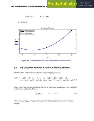
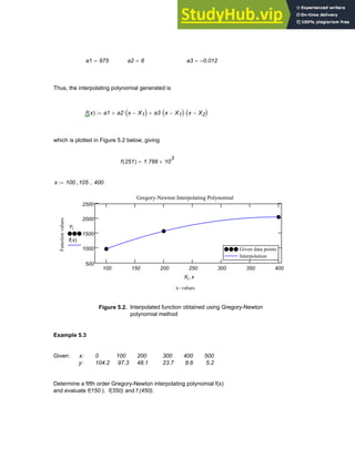
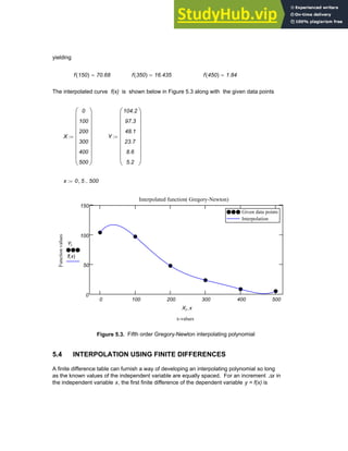
Example 5.2 -
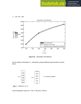
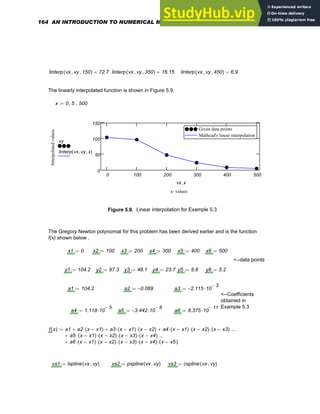
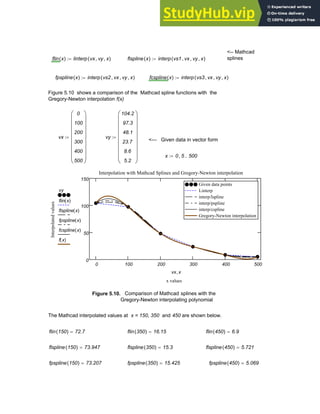
Given three data points: X: 100 200 400
Y: 975 1575 2054
Determine the Gregory -Newton Polynomial f(x) and evaluate f(251)
The form of this polynomial will be :
y = f(x) = a1 + a2(x-X1 + a3(x-X1)(x-X2)
with a1 = Y1
a2 = (Y2-Y1) / (X2-X1)
a3 = [ Y3- a1 -a2(X3-X1)] /[ (X3-X1)(X3-X2)]
The data is put in in vector form as follows.
X
100
200
400
⎛
⎜
⎜
⎜
⎝
⎞
⎟
⎟
⎟
⎠
:= Y
975
1575
2054
⎛
⎜
⎜
⎜
⎝
⎞
⎟
⎟
⎟
⎠
:=
and the coefficients a1, a2 and a3 are computed using
a1 Y1
:= a2
Y2 Y1
−
X2 X1
−
:= a3
Y3 a1
− a2 X3 X1
−
( )
⋅
−
X3 X1
−
( ) X3 X2
−
( )
⋅
:=
146 AN INTRODUCTION TO NUMERICAL METHODS USING MATHCAD](https://image.slidesharecdn.com/anintroductiontonumericalmethodsusingmathcadmathcadrelease14-230805170449-0ea94cc2/85/AN-INTRODUCTION-TO-NUMERICAL-METHODS-USING-MATHCAD-Mathcad-Release-14-156-320.jpg)

![Δf = f(x+Δx)- f(x) (5.12)
The second finite difference is
Δ 2 f = Δ[Δf] =[f(x+2Δx)-f(x+Δx)]-[f(x+Δx)- f(x)] (5.13)
Similarly, the (n-1)th finite difference will be
Δn f = Δ[Δ n-1 f ] (5.14)
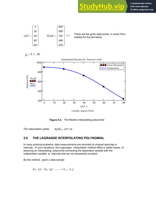
The finite differences as derived above are arranged in a table as shown in Table 5.1 which
can be used to generate an interpolating polynomial, as will be demonstrated later.
TABLE 5.1
Table of finite differences
--------------------------------------------------------------------------------------------------------------------------------
x f x
( ) Δf Δ
2
f Δ
3
f Δ
n
f
-------------------------------------------------------------------------------------------------------------------------------
x f x
( )
Δf x
( )
x Δx
+ f x Δx
+
( ) Δ
2
f x
( )
Δf x Δx
+
( ) Δ
3
f x
( )
x 2 Δx
⋅
+ f x 2 Δx
⋅
+
( ) Δ
2
f x Δx
+
( )
Δf x 2 Δx
⋅
+
( )
x 3 Δx
⋅
+ f x 3 Δx
⋅
+
( )
------------------------------------------------------------------------------------------------------------------------------------
150 AN INTRODUCTION TO NUMERICAL METHODS USING MATHCAD](https://image.slidesharecdn.com/anintroductiontonumericalmethodsusingmathcadmathcadrelease14-230805170449-0ea94cc2/85/AN-INTRODUCTION-TO-NUMERICAL-METHODS-USING-MATHCAD-Mathcad-Release-14-160-320.jpg)


![fpspline 415
( ) 962.582
= fcspline 415
( ) 955.728
=
5.9. APPLICATIONS IN NUMERICAL INTERPOLATION
In the examples that follow, data from various practical areas such as design of
machinery, noise control and vibration analysis, is utilized in interpolation procedure s to
generate function values at points other than the given data points.
5.9.1. Stress-Strain Data for Titanium
The stress versus strain data given in the table below is obtained from a tensile test of
annealed A-40 titanium [ 18 ]. A cubic spline can be developed using Mathcad as follows
and the stresses interpolated for any values of strain in the range provided.
The cubic spline interpolation generated together with the given data points is presented in
Figure 5.12. Notice that the spline generated passes through all the given data points as is
expected of an interpolating polynomial.
Strain (in/in) Stress (kpsi)
<--Given stress versus strain data
σ
0
5
10
15
20
25
30
34.9
39.9
44.9
49.9
60.9
73.3
78.2
86.2
94.5
98.7
118.2
⎛
⎜
⎜
⎜
⎜
⎜
⎜
⎜
⎜
⎜
⎜
⎜
⎜
⎜
⎜
⎜
⎜
⎜
⎜
⎜
⎜
⎜
⎜
⎜
⎜
⎜
⎝
⎞
⎟
⎟
⎟
⎟
⎟
⎟
⎟
⎟
⎟
⎟
⎟
⎟
⎟
⎟
⎟
⎟
⎟
⎟
⎟
⎟
⎟
⎟
⎟
⎟
⎟
⎠
:=
ε
0
0.00030
0.00060
0.00090
0.00120
0.00175
0.00220
0.00285
0.00349
0.00469
0.00698
0.01610
0.04807
0.07676
0.14364
0.26677
0.34470
0.72202
⎛
⎜
⎜
⎜
⎜
⎜
⎜
⎜
⎜
⎜
⎜
⎜
⎜
⎜
⎜
⎜
⎜
⎜
⎜
⎜
⎜
⎜
⎜
⎜
⎜
⎜
⎝
⎞
⎟
⎟
⎟
⎟
⎟
⎟
⎟
⎟
⎟
⎟
⎟
⎟
⎟
⎟
⎟
⎟
⎟
⎟
⎟
⎟
⎟
⎟
⎟
⎟
⎟
⎠
:=
Vε ε
:= Vσ σ
:=
Vs cspline Vε Vσ
,
( )
:=
168 AN INTRODUCTION TO NUMERICAL METHODS USING MATHCAD](https://image.slidesharecdn.com/anintroductiontonumericalmethodsusingmathcadmathcadrelease14-230805170449-0ea94cc2/85/AN-INTRODUCTION-TO-NUMERICAL-METHODS-USING-MATHCAD-Mathcad-Release-14-178-320.jpg)
![fspline ε
( ) interp Vs Vε
, Vσ
, ε
,
( )
:= <-- Generates a cubic spline function for given data
fspline 0.004
( ) 42.699
=
<-- interpolated values of stress at strains of 0.004 and 0.65
fspline 0.65
( ) 114.503
=
i 1 18
..
:= ε 0 0.00010
, 0.722
..
:=
1 .10
4
1 .10
3
0.01 0.1 1
1
10
100
1 .10
3
fspline ε
( )
Vσi
ε Vεi
,
Figure 5.12. Mathcad cubic spline for given stress-strain data
5.9.2. Notch Sensitivity of Aluminum
The fatigue stress concentration factor K f is used with the nominal stress σ 0 to compute
the maximum resulting stress σ max at a discontinuity in a machine part via the following
relationship [18] .
σmax Kf σ0
⋅
= (5.31)
The fatigue stress concentration factor K f , which is, in fact , just a reduced value of the
geometrical stress concentration factor K t, is a function of the sensitivity of the material of
which the part is made to notches ( known as notch sensitivity q ). These quantities are
connected by the following relationship .
Chapter 5: Numerical Interpolation 169](https://image.slidesharecdn.com/anintroductiontonumericalmethodsusingmathcadmathcadrelease14-230805170449-0ea94cc2/85/AN-INTRODUCTION-TO-NUMERICAL-METHODS-USING-MATHCAD-Mathcad-Release-14-179-320.jpg)

![fspline 0.13
( ) 0.787
= fspline 0.15
( ) 0.813
= f 0.15
( ) 0.814
= fspline 0.15
( ) 0.813
=
r 0.015 0.016
, 0.16
..
:= i 1 7
..
:=
0.02 0.04 0.06 0.08 0.1 0.12 0.14 0.16
0.2
0.4
0.6
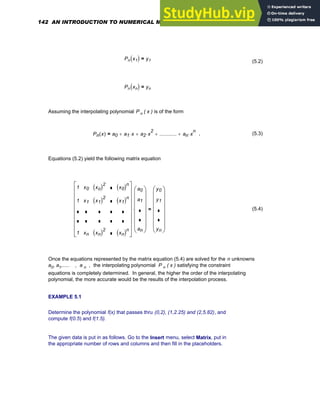
0.8
Given data points
Interpolation by undet coeff method
Mathcad cubic spline interpolation
Given data points
Interpolation by undet coeff method
Mathcad cubic spline interpolation
Mathcad interpolation/ notch sensitivity
Notch radius, r, inches
Notch
sensitivity,
q
Vqi
f r
( )
fspline r
( )
Vri r
,
Figure 5.13. Interpolation of notch sensitivity data
5.9.3 Speech Interference Level
In the field of Noise and Vibration Control, it often becomes necessary to determine the
effect of steady background noise on speech communication in a given setting. The
preferred speech interference level (PSIL) was established in an effort to study this effect
under the constraint that speech sounds would not be allowed to be reflected back to the
listener [ 2, 10 ]. For effective communication at a given voice level , the maximum
distance that there can be between the speaker and the listener is a function of the
preferred speech interference level existing at the location. The following data which is
provided for communication at the level of a normal male voice can be utilized in an
interpolation scheme to determine the maximum PSIL permitted for a given distance
between the speaker and the listener.
Dist (ft) 0 2 4 6 8 10 12
PSIL(dB) 83 62.5 56 52.5 50 47.5 46.5
172 AN INTRODUCTION TO NUMERICAL METHODS USING MATHCAD](https://image.slidesharecdn.com/anintroductiontonumericalmethodsusingmathcadmathcadrelease14-230805170449-0ea94cc2/85/AN-INTRODUCTION-TO-NUMERICAL-METHODS-USING-MATHCAD-Mathcad-Release-14-182-320.jpg)


![0 2 4 6 8 10 12
40
50
60
70
80
90
Given data points
Gregory-Newton interpolation
Mathcad's interp/cspline
Given data points
Gregory-Newton interpolation
Mathcad's interp/cspline
Interpolation- speech communication
Distance from speaker to listener (ft)
Preferred
speech
interference
level
(
dB
Vyi
f x
( )
fspline x
( )
Vxi x
,
Figure 5.14. Interpolation of speech communication data
5.9.4. Load-Deflection Data for Elastomeric Mounts
Elastomeric mounts are employed when small electrical and mechanical devices have to be
isolated from high forcing frequencies [ 9, 10 ]. They are especially useful in the protection of
delicate electronic instruments . Mount performance characteristics in the form of load
versus static deflection data are provided by manufacturers of vibration control products to
enable a designer to select an appropriate isolator for a given application.
The following data is available for an elastomeric mount.
Deflection (cm): 0 0 0.02 0.04 0.06 0.08 0.10
Load (N): 5 11 17.5 23.5 28 30.5
There are six data points prescribed. Thus, if a Lagrangian interpolating polynomial is to be
generated, it will be of order 5, having the form
L D
( )
1
6
i
wi D
( ) . Li
⋅
( )
∑
=
=
where
Chapter 5: Numerical Interpolation 175](https://image.slidesharecdn.com/anintroductiontonumericalmethodsusingmathcadmathcadrelease14-230805170449-0ea94cc2/85/AN-INTRODUCTION-TO-NUMERICAL-METHODS-USING-MATHCAD-Mathcad-Release-14-185-320.jpg)
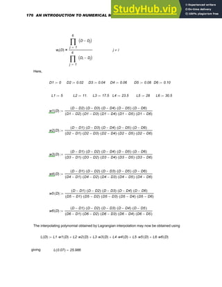
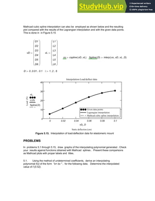

![5.7. The amplitude of vibration of an automobile in the vertical direction, after passing over
a road bump is found to be as follows.
Time, t (seconds) 0 0.65 1.30 1.95
Amplitude, A (mm) 5.25 2.50 0.80 0.40
Using the Gregory-Newton method, compute the amplitude for t = 1.80 seconds.
5.8. The Charpy test [ 18 ] provides material toughness data under dynamic conditions.
In this test, which is helpful in comparing several materials and in determining
low-temperature brittleness and impact strength, the specimen is struck by a pendulum
released from a fixed height and the energy absorbed by the specimen, termed the impact
value , computed from the height of the swing after fracture. The following table gives the
impact value, V, as a function of temperature, T, for a certain material. Using the
Gregory-Newton method, derive an interpolating polynomial and estimate V for T = -25 deg.
F and - 75 deg. F
T (deg F) -200 -150 -100 -50 0
V (ft-lbs) 0 1.5 3 10 35
5.9. The data in the following table are the distances traveled by a motorcycle, which was
stationary at time t = 0, for selected times.
time, t (seconds) 0 2 4 6 8 10
Distance, D (ft) 0 10 50 150 330 610
Generate a finite-difference table and obtain an interpolating polynomial using Newton's
method. Estimate the distance D traveled at t = 7 seconds.
5.10. For the given data, generate both a finite-difference table and an interpolating
polynomial.
Angle, θ, (degrees) Cosine (θ)
0 1.00000
10 0.98481
20 0.93969
30 0.86603
40 0.76604
50 0.64279
60 0.50000
Evaluate the error of the estimated value of cos (25 degrees). The true value is given to be
0.90631.
Chapter 5: Numerical Interpolation 179](https://image.slidesharecdn.com/anintroductiontonumericalmethodsusingmathcadmathcadrelease14-230805170449-0ea94cc2/85/AN-INTRODUCTION-TO-NUMERICAL-METHODS-USING-MATHCAD-Mathcad-Release-14-189-320.jpg)
![5.11. The following data gives the notch sensitivity , q , of a steel as a functionof the
notch radius , r [ 18 ]. Compute a finite-difference table and derive an interpolating
polynomial by Newton's method. Estimate q for r = 0.11 inches.
q 0.45 0.65 0.75 0.78 0.785
r ( in) 0.01 0.05 0.09 0.13 0.17
5.12. The deflection, δ, of a structure under loading is measured at a point for four different
values of the applied force, F. The measured data is as follows.
F (kn) 0.50 1.50 2.0 2.50
δ (cm) 3.0 5.2 7.3 10.5
Using Lagrangian interpolation , compute the deflection, δ, for F = 2.2 kN.
5.13. When a vibration problem is solved with nonlinearities included, the natural
frequencies of vibration become dependent on the amplitudes of vibration [ 9,16,20,21 ].
The following table relates the nonlinear natural frequency / linear natural frequency ratio,
r, of a rotating blade vibrating in the plane of rotation to its vibration amplitude , A.
A (in) 10 8.5 5 0
r (%) 99.9325 99.9575 99.9921 100
Derive a Lagrange interpolating polynomial and compute r for A = 4.25 in .
5.14. The behavior of a mooring line employed to control the excursions of a floating
ocean structure resembles that of a nonlinear spring with tension-displacement
characteristics which depend upon its length, weight, elastic properties, anchor holding
capacities and water depth [ 22 ]. In the table below, the horizontal component of mooring
line tension , H, is given as a function of the horizontal distance, X, between the ends of the
line.
X (ft) 440 470 485 492.5 495 498
H (Kips)0 5 10 42 150 440
Using Lagrangian interpolation, generate an interpolating polynomial and compute H for
X= 487 ft.
180 AN INTRODUCTION TO NUMERICAL METHODS USING MATHCAD](https://image.slidesharecdn.com/anintroductiontonumericalmethodsusingmathcadmathcadrelease14-230805170449-0ea94cc2/85/AN-INTRODUCTION-TO-NUMERICAL-METHODS-USING-MATHCAD-Mathcad-Release-14-190-320.jpg)
![5.15. The following table gives the pressure (P) versus temperature (T) relationship in the
liquid-vapor region for water [ 17 ]
T(deg Kelvin) 403.15 453.15 503.15 553.15 633.15
P (MPa) 0.2701 1.0021 2.795 6.412 18.651
Using Lagrangian interpolation, generate an interpolating polynomial and estimate P for T=
525 deg. K.
5.16. While the value of the endurance limit, S end , of a material is based on its
tensile strength, S ult , it is also dependent on the condition of its surface[19 ]. The following
data relates to a machined , unnotched specimen subjected to reversed bending.
S ult ( kpsi): 60 80 100 140 180 220
S end (kpsi): 22 30 38 50 60 64
Develop linear and cubic splines using linterp and interp for the above data. Also ,
graph the functions generated with proper labels and a title.
Chapter 5: Numerical Interpolation 181](https://image.slidesharecdn.com/anintroductiontonumericalmethodsusingmathcadmathcadrelease14-230805170449-0ea94cc2/85/AN-INTRODUCTION-TO-NUMERICAL-METHODS-USING-MATHCAD-Mathcad-Release-14-191-320.jpg)

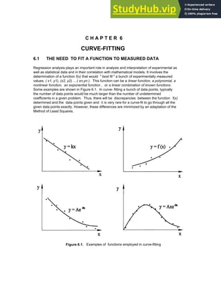

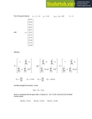
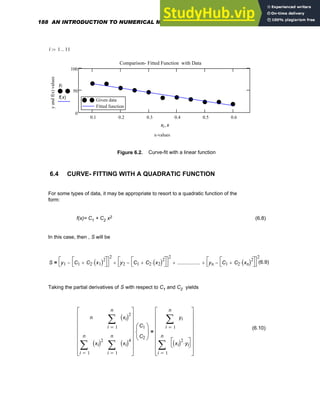
![which can be solved for the C's using algebraic or matrix methods or by accessing the
Mathcad function lsolve. The above can be expressed as
[M]{C} = {A}, (6.11)
where
(6.12)
M
n
1
n
i
xi
( )2
∑
=
1
n
i
xi
( )2
∑
=
1
n
i
xi
( )4
∑
=
⎡
⎢
⎢
⎢
⎢
⎢
⎢
⎣
⎤
⎥
⎥
⎥
⎥
⎥
⎥
⎦
= , A
1
n
i
yi
∑
=
1
n
i
xi
( )2
yi
⋅
⎡
⎣
⎤
⎦
∑
=
⎡
⎢
⎢
⎢
⎢
⎢
⎢
⎣
⎤
⎥
⎥
⎥
⎥
⎥
⎥
⎦
=
Example 6.2
A data set is given below .
x y
0.5 0.51
1.0 2.35
1.5 7.54
2.0 13.23
2.5 17.65
3.0 24.21
3.5 28.94
4.0 37.63
4.5 58.32
5.0 63.21
Determine the quadratic function that will best fit the data given
Put in the given data :
i 1 2
, 10
..
:= x1 0.5
:= xi 1
+ xi 0.5
+
:= n 10
:=
y1 0.51
:= y2 2.35
:= y3 7.54
:= y4 13.23
:= y5 17.65
:=
y6 24.21
:= y7 28.94
:= y8 37.63
:= y9 58.32
:= y10 63.21
:=
In this problem, the [M} and {A} matrices are
Chapter 6: Curve-Fitting 189](https://image.slidesharecdn.com/anintroductiontonumericalmethodsusingmathcadmathcadrelease14-230805170449-0ea94cc2/85/AN-INTRODUCTION-TO-NUMERICAL-METHODS-USING-MATHCAD-Mathcad-Release-14-199-320.jpg)

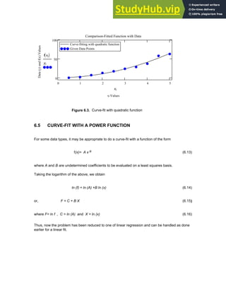
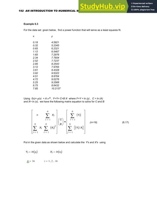
![x
0.18
0.32
0.65
1.12
1.65
2.34
2.52
2.85
3.12
3.61
3.92
4.51
4.72
5.25
6.75
7.85
⎛
⎜
⎜
⎜
⎜
⎜
⎜
⎜
⎜
⎜
⎜
⎜
⎜
⎜
⎜
⎜
⎜
⎜
⎜
⎜
⎜
⎜
⎝
⎞
⎟
⎟
⎟
⎟
⎟
⎟
⎟
⎟
⎟
⎟
⎟
⎟
⎟
⎟
⎟
⎟
⎟
⎟
⎟
⎟
⎟
⎠
:= y
4.5921
5.2345
6.2321
6.5467
7.2976
7.7654
7.7237
8.2543
7.9765
8.4328
9.6322
8.8764
9.0276
9.2568
8.6432
10.2137
⎛
⎜
⎜
⎜
⎜
⎜
⎜
⎜
⎜
⎜
⎜
⎜
⎜
⎜
⎜
⎜
⎜
⎜
⎜
⎜
⎜
⎜
⎝
⎞
⎟
⎟
⎟
⎟
⎟
⎟
⎟
⎟
⎟
⎟
⎟
⎟
⎟
⎟
⎟
⎟
⎟
⎟
⎟
⎟
⎟
⎠
:=
Yi ln yi
( )
:= Xi ln xi
( )
:=
Equation 6.17 is: [D] { K} = {P}, where
P
1
n
i
Yi
( )
∑
=
1
n
i
Yi
( ) Xi
⋅
⎡
⎣ ⎤
⎦
∑
=
⎡
⎢
⎢
⎢
⎢
⎢
⎢
⎣
⎤
⎥
⎥
⎥
⎥
⎥
⎥
⎦
:=
D
n
1
n
i
Xi
∑
=
1
n
i
Xi
∑
=
1
n
i
Xi
( )2
∑
=
⎡
⎢
⎢
⎢
⎢
⎢
⎢
⎣
⎤
⎥
⎥
⎥
⎥
⎥
⎥
⎦
:=
and {K} is the vector of unknown coefficients C and B
The constants C and B can be obtained using lsolve as shown below, and then the coefficients
A and B of the power function can be calculated
K lsolve D P
,
( )
:= K
1.883
0.2
⎛
⎜
⎝
⎞
⎟
⎠
= <------ This means: C= 1.883 and B = 0.2
C K1
:= B K2
:= C 1.883
= B 0.2
=
Chapter 6: Curve-Fitting 193](https://image.slidesharecdn.com/anintroductiontonumericalmethodsusingmathcadmathcadrelease14-230805170449-0ea94cc2/85/AN-INTRODUCTION-TO-NUMERICAL-METHODS-USING-MATHCAD-Mathcad-Release-14-203-320.jpg)
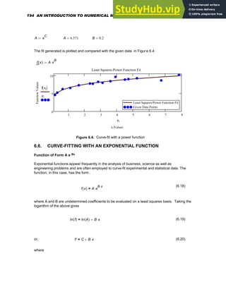

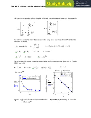
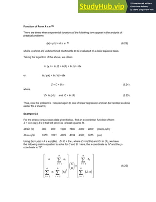
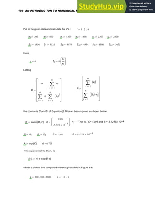
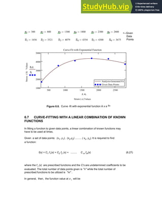
![f xi
( )
1
m
j
Cj fj xi
( )
⋅
⎡
⎣ ⎤
⎦
∑
=
= (6.28)
In this case, the sum of the squares of the deviations from the true values y i will be:
s y1 f x1
( )
−
( )2
y2 f x2
( )
−
( )2
+ ......................
+ yn f xn
( )
−
( )2
+
=
(6.29)
For S to be a minimum , the partial derivatives of S with respect to C1, C2 ....... C m
must be zero and the second partials must be positive. These requirements lead to the following
matrix equation in the unknowns, C 1, C2 ...... C m
[M] {C} = {L} (6.30)
where
C
C1
C2
Cm
⎛
⎜
⎜
⎜
⎜
⎜
⎜
⎜
⎜
⎝
⎞
⎟
⎟
⎟
⎟
⎟
⎟
⎟
⎟
⎠
:= , L
1
n
i
f1 xi
( )
⎡
⎣ ⎤
⎦ yi
( )
⋅
⎡
⎣ ⎤
⎦
∑
=
1
n
i
f2 xi
( )
⎡
⎣ ⎤
⎦ yi
( )
⋅
⎡
⎣ ⎤
⎦
∑
=
1
n
i
fm xi
( )
⎡
⎣ ⎤
⎦ yi
( )
⋅
⎡
⎣ ⎤
⎦
∑
=
⎡
⎢
⎢
⎢
⎢
⎢
⎢
⎢
⎢
⎢
⎢
⎢
⎢
⎢
⎢
⎢
⎣
⎤
⎥
⎥
⎥
⎥
⎥
⎥
⎥
⎥
⎥
⎥
⎥
⎥
⎥
⎥
⎥
⎦
:= , and
200 AN INTRODUCTION TO NUMERICAL METHODS USING MATHCAD](https://image.slidesharecdn.com/anintroductiontonumericalmethodsusingmathcadmathcadrelease14-230805170449-0ea94cc2/85/AN-INTRODUCTION-TO-NUMERICAL-METHODS-USING-MATHCAD-Mathcad-Release-14-210-320.jpg)

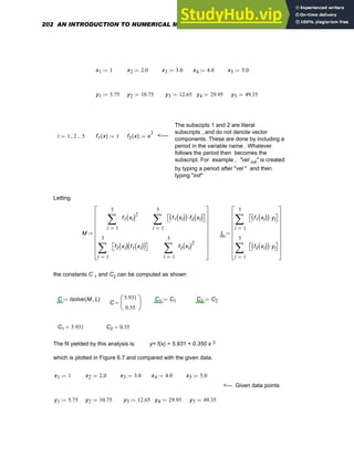
![yanal x
( ) C1 f1 x
( )
⋅ C2 f2 x
( )
⋅
+
:= <--- Curve-fit generated by analysis
yanal 1
( ) 6.281
= yanal 2
( ) 8.733
=
<---y-values generated by curve-fit
yanal 3
( ) 15.386
=
z 1 1.1
, 5
..
:= i 1 5
..
:=
1 2 3 4 5
0
20
40
60
Results of Analysis
Given data points
Results of Analysis
Given data points
Analysis - Generated Fit/ Given Data
X- Values
Y-
Values
yanal z
( )
yi
z xi
,
Figure 6.7. Curve-fit with a linear combination of known functions
6.8 CURVE-FITTING WITH POLYNOMIALS
If an mth order polynomial seems to be a good fit to the data points given, the procedure used
in fitting a linear combination of known functions can still be resorted to. In this case,
f 1 ( x) = 1, f 2 (x) = x , f 3 ( x ) = x 2, f 4 ( x ) = x 3 , ............. ,
f m+1 (x ) = x m
(6.31)
f(x) = C1 f 1 (x ) + C 2 f 2 ( x ) +....................... C m+1 f m+1 ( x ) (6.32)
in which the C 's must be solved for using
[M] {C} = {L} (6.33)
Chapter 6: Curve-Fitting 203](https://image.slidesharecdn.com/anintroductiontonumericalmethodsusingmathcadmathcadrelease14-230805170449-0ea94cc2/85/AN-INTRODUCTION-TO-NUMERICAL-METHODS-USING-MATHCAD-Mathcad-Release-14-213-320.jpg)
![where
C
C1
C2
Cm 1
+
⎛
⎜
⎜
⎜
⎜
⎜
⎜
⎝
⎞
⎟
⎟
⎟
⎟
⎟
⎟
⎠
:=
M
n
1
n
i
xi
∑
=
1
n
i
xi
( )2
∑
=
1
n
i
xi
( )m
∑
=
1
n
i
xi
∑
=
1
n
i
xi
( )2
∑
=
1
n
i
xi
( )m
∑
=
1
n
i
xi
( )m 1
+
∑
=
1
n
i
xi
( )m 2
+
∑
=
1
n
i
xi
( )2 m
⋅
∑
=
⎡
⎢
⎢
⎢
⎢
⎢
⎢
⎢
⎢
⎢
⎢
⎢
⎢
⎢
⎢
⎢
⎢
⎣
⎤
⎥
⎥
⎥
⎥
⎥
⎥
⎥
⎥
⎥
⎥
⎥
⎥
⎥
⎥
⎥
⎥
⎦
:= L
1
n
i
yi
∑
=
1
n
i
xi yi
⋅
( )
∑
=
1
n
i
xi
( )m
yi
⋅
⎡
⎣
⎤
⎦
∑
=
⎡
⎢
⎢
⎢
⎢
⎢
⎢
⎢
⎢
⎢
⎢
⎢
⎢
⎢
⎣
⎤
⎥
⎥
⎥
⎥
⎥
⎥
⎥
⎥
⎥
⎥
⎥
⎥
⎥
⎦
:=
,
where the ( x i, y i ) are the "n" given data points.
Example 6.7.
Given the data points
x: 0 1 2 3 4 5
y: 0 8.47 17.48 19.57 14.69 11.23
Obtain a curve-fit of the form y x
( ) f x
( )
= C1 C2 x
⋅
+ C3 x
2
⋅
+
=
Here, n = 6 and m = 2 and the matrix equation to be solved is
[M]{C} = {L}
204 AN INTRODUCTION TO NUMERICAL METHODS USING MATHCAD](https://image.slidesharecdn.com/anintroductiontonumericalmethodsusingmathcadmathcadrelease14-230805170449-0ea94cc2/85/AN-INTRODUCTION-TO-NUMERICAL-METHODS-USING-MATHCAD-Mathcad-Release-14-214-320.jpg)
![where [M] is a known 3x3 matrix and {L} is a known column vector as shown below. The
The column vector {C} , which involves the undetermined coefficients, is
C1
C2
C3
⎛
⎜
⎜
⎜
⎝
⎞
⎟
⎟
⎟
⎠
The given data is
n 6
:= x1 0
:= x2 1
:= x3 2
:= x4 3
:= x5 4
:= x6 5
:=
y1 0
:= y2 8.47
:= y3 17.48
:= y4 19.57
:= y5 14.69
:= y6 11.23
:=
The matrices M and L are
L
1
n
i
yi
∑
=
1
n
i
xi yi
⋅
( )
∑
=
1
n
i
xi
( )2
yi
⋅
⎡
⎣
⎤
⎦
∑
=
⎡
⎢
⎢
⎢
⎢
⎢
⎢
⎢
⎢
⎢
⎢
⎣
⎤
⎥
⎥
⎥
⎥
⎥
⎥
⎥
⎥
⎥
⎥
⎦
:=
M
n
1
n
i
xi
∑
=
1
n
i
xi
( )2
∑
=
1
n
i
xi
∑
=
1
n
i
xi
( )2
∑
=
1
n
i
xi
( )3
∑
=
1
n
i
xi
( )2
∑
=
1
n
i
xi
( )3
∑
=
1
n
i
xi
( )4
∑
=
⎡
⎢
⎢
⎢
⎢
⎢
⎢
⎢
⎢
⎢
⎢
⎣
⎤
⎥
⎥
⎥
⎥
⎥
⎥
⎥
⎥
⎥
⎥
⎦
:=
The unknown constants are determined below using lsolve
C lsolve M L
,
( )
:= C
0.444
−
12.484
2.057
−
⎛
⎜
⎜
⎝
⎞
⎟
⎟
⎠
=
C1 C1
:= C2 C2
:= C3 C3
:=
C1 0.444
−
= C2 12.484
= C3 2.057
−
=
The polynomial fitting the given data , then, is
Chapter 6: Curve-Fitting 205](https://image.slidesharecdn.com/anintroductiontonumericalmethodsusingmathcadmathcadrelease14-230805170449-0ea94cc2/85/AN-INTRODUCTION-TO-NUMERICAL-METHODS-USING-MATHCAD-Mathcad-Release-14-215-320.jpg)
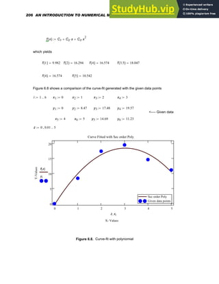

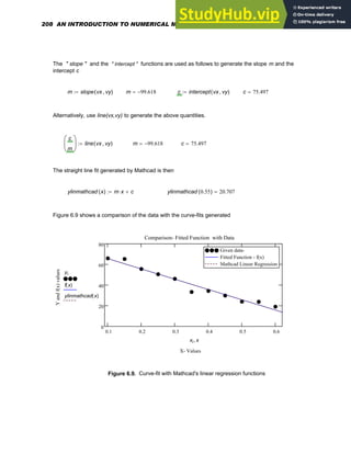

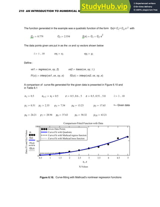

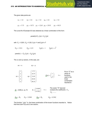
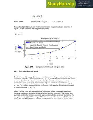

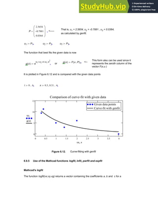
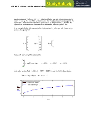

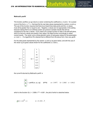
![0 1 2 3 4 5 6 7
0
2000
4000
Given data points
Mathcad's pwrfit
Given data points
Mathcad's pwrfit
vy
f x
( )
vx x
,
Mathcad's expfit
The function expfit(vx,vy, [vg]) returns a vector containing the coefficients a, b and c for an
exponential curve of the form A exp (b x ) + C that best fits the real data values represented by
vectors vx and vy. The use of this function requires that there be at least three data points and the
vx values must all be greater than or equal to zero. If a fit has be done on data that has negative
x-values, then the data must be shifted to the positive axis. . Otherwise, a curve-fit with erroneous
values may be generated. The vector vg is a three-element vector of real guess values for the
parameters A, b and C, but it is optional, and does not have to be used. However, if it is not
used, then expfit generates a guess that fits a line to the logs of vy. If an exponential fit is
desired that is different from the above form, then use genfit .
For the data points represented by the vectors vx and vy as given below, and with the use of the
vector vg of guess values shown for the coefficients a, b and c ,.
vg
3
2
10
⎛
⎜
⎜
⎝
⎞
⎟
⎟
⎠
:=
vx
0
1
2
3
4
5
6
7
8
⎛
⎜
⎜
⎜
⎜
⎜
⎜
⎜
⎜
⎜
⎜
⎜
⎝
⎞
⎟
⎟
⎟
⎟
⎟
⎟
⎟
⎟
⎟
⎟
⎟
⎠
:= vy
21
24.892
31.31
41.89
59.334
88.095
135.513
213.693
342.589
⎛
⎜
⎜
⎜
⎜
⎜
⎜
⎜
⎜
⎜
⎜
⎜
⎝
⎞
⎟
⎟
⎟
⎟
⎟
⎟
⎟
⎟
⎟
⎟
⎟
⎠
:=
the curve-fit returned by Mathcad's expfit is defined by
Chapter 6: Curve-Fitting 219](https://image.slidesharecdn.com/anintroductiontonumericalmethodsusingmathcadmathcadrelease14-230805170449-0ea94cc2/85/AN-INTRODUCTION-TO-NUMERICAL-METHODS-USING-MATHCAD-Mathcad-Release-14-229-320.jpg)
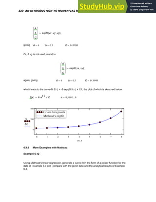

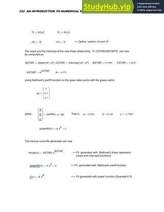
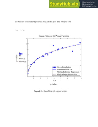
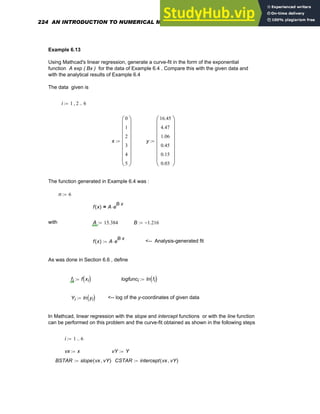
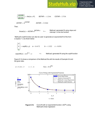

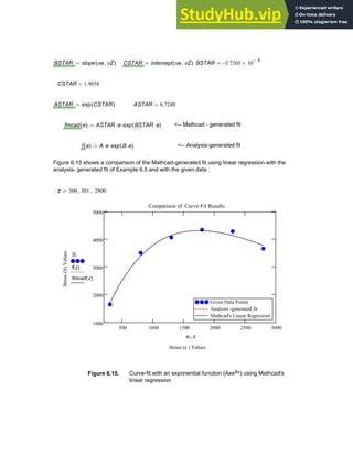
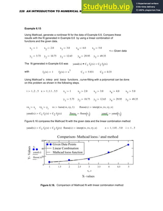
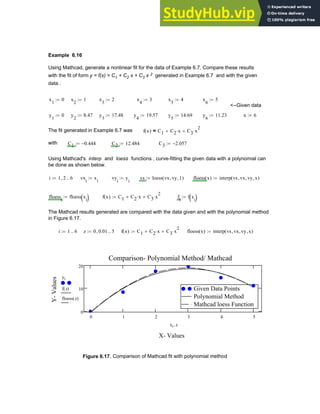
![Example 6.17
Fit the data points :
x: 0.1 0.2 0.3 0.4 0.5 0.6 0.7 0.8
y: 0.59 0.83 0.90 0.95 1.02 1.43 1.75 3.15
with a function of the form : y = C1 f 1 (x ) + C2 f 2 ( x) +C 3 f 3(x) + C4 f4 (x) where
f 1 (x ) = 1 , f 2 ( x ) = x2 , f 3 ( x) = sin (2x) , f 4 ( x) = exp( 0.95x )
In this case, we have the following matrix equation
[M] {C} = {L} ,
where {C} is the column vector of unknown coefficients C1, C2, C3 and C4 , and [M] and {L} are
known matrices as generated below.
The given data is
N 8
:=
x1 0.1
:= x2 0.2
:= x3 0.3
:= x4 0.4
:= x5 0.5
:= x6 0.6
:= x7 0.7
:= x8 0.8
:=
y1 0.59
:= y2 0.83
:= y3 0.90
:= y4 0.95
:= y5 1.02
:= y6 1.43
:= y7 1.75
:= y8 3.15
:=
i 1 2
, 8
..
:= f1 x
( ) 1
:= f2 x
( ) x
2
:= <--- The subscipts 1 and 2 are literal
subscripts , and do not denote
vector components. These are
done by including a period in the variable
name . Whatever follows the period then
becomes the subscript. For
example , "vel init" is created by typing
a period after "vel" and then typing "init"
f3 x
( ) sin 2 x
⋅
( )
:=
f4 x
( ) exp 0.95 x
⋅
( )
:=
In this case, the M and L matrices are
230 AN INTRODUCTION TO NUMERICAL METHODS USING MATHCAD](https://image.slidesharecdn.com/anintroductiontonumericalmethodsusingmathcadmathcadrelease14-230805170449-0ea94cc2/85/AN-INTRODUCTION-TO-NUMERICAL-METHODS-USING-MATHCAD-Mathcad-Release-14-240-320.jpg)
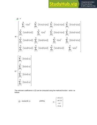
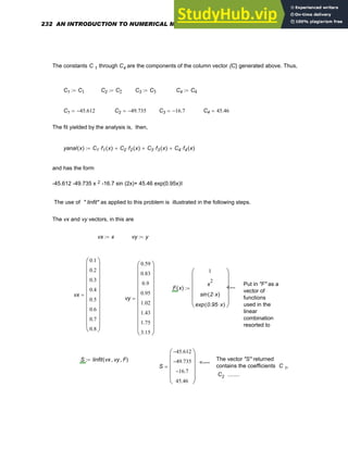
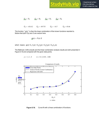
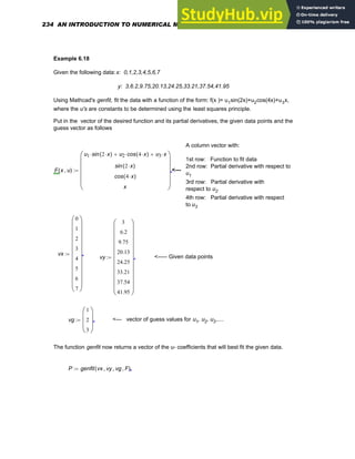
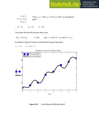
![6.10 APPLICATIONS IN CURVE-FITTING
In the world of engineering, science, and business, it is very common to see a function in
the form of data prescribed at many points, and in addition, there may also be
considerable scatter in the available data . The methods discussed in the earlier sections
of this chapter will now be used to generate appropriate curve-fits to actual data from
several practical applications.
6.10.1 Fatigue Failure Curve for Loading in the Finite Life Range
The fatigue failure curve of a material provides useful information pertinent to the design of
machinery for finite life [ 19 ]. It is essentially a relationship between the completely
reversed applied stress, S, and fatigue life, L , which is measured in terms of the number
of stress reversals to failure.
The following data pertains to a steel with an endurance limit of 40 kpsi and an ultimate
strength of 90 kpsi. It is required to curve-fit the data with a suitable function.
L ( million cycles) Stress (kpsi)
vL
0.02
0.03
0.04
0.05
0.075
0.1
0.2
0.4
0.6
0.8
1.0
1.1
1.2
1.3
⎛
⎜
⎜
⎜
⎜
⎜
⎜
⎜
⎜
⎜
⎜
⎜
⎜
⎜
⎜
⎜
⎜
⎜
⎜
⎝
⎞
⎟
⎟
⎟
⎟
⎟
⎟
⎟
⎟
⎟
⎟
⎟
⎟
⎟
⎟
⎟
⎟
⎟
⎟
⎠
:= vS
80
70
65
61
57
55
50
45
42
40.5
40.1
40
39.9
39.85
⎛
⎜
⎜
⎜
⎜
⎜
⎜
⎜
⎜
⎜
⎜
⎜
⎜
⎜
⎜
⎜
⎜
⎜
⎜
⎝
⎞
⎟
⎟
⎟
⎟
⎟
⎟
⎟
⎟
⎟
⎟
⎟
⎟
⎟
⎟
⎟
⎟
⎟
⎟
⎠
:=
From the plot of the given data shown in Figure 6.20, it appears that a power function would
furnish a reasonable curve-fit. This has the form
S(L)= A*LB ,
236 AN INTRODUCTION TO NUMERICAL METHODS USING MATHCAD](https://image.slidesharecdn.com/anintroductiontonumericalmethodsusingmathcadmathcadrelease14-230805170449-0ea94cc2/85/AN-INTRODUCTION-TO-NUMERICAL-METHODS-USING-MATHCAD-Mathcad-Release-14-246-320.jpg)
![where A and B are undetermined coefficients to be evaluated on a least squares basis.
i 1 14
..
:=
0 0.2 0.4 0.6 0.8 1 1.2
40
60
80
Given Data
Given Data
Given Data Points
Given L- values (million cycles )
Given
S-
values
(kpsi)
vSi
vLi
Figure 6.20. Fatigue life data
Using S(L) = A L B , Sstar= C+ B . Lstar , where Lstar= ln (L) , C = ln (A) and
Sstar= ln (S), the matrix equation [D]{X} = {P} is obtained , where {X} is the column vector
containing the unknowns C and B.
n 14
:= Sstar ln vS
( )
:= Lstar ln vL
( )
:= D X
⋅ P
=
D
n
1
n
i
Lstar i
∑
=
1
n
i
Lstar i
∑
=
1
n
i
Lstar i
( )2
∑
=
⎡
⎢
⎢
⎢
⎢
⎢
⎢
⎣
⎤
⎥
⎥
⎥
⎥
⎥
⎥
⎦
:=
P
1
n
i
Sstari
∑
=
1
n
i
Sstari Lstar i
⋅
( )
∑
=
⎡
⎢
⎢
⎢
⎢
⎢
⎢
⎣
⎤
⎥
⎥
⎥
⎥
⎥
⎥
⎦
:=
The unknown constants C and B can be computed using lsolve as shown below
K lsolve D P
,
( )
:= K
3.684
0.155
−
⎛
⎜
⎝
⎞
⎟
⎠
= <------Thus, C= 3.684 and B = -0.155
C K1
:= B K2
:= C 3.684
= B 0.155
−
= A e
C
:= A 39.808
=
Chapter 6: Curve-Fitting 237](https://image.slidesharecdn.com/anintroductiontonumericalmethodsusingmathcadmathcadrelease14-230805170449-0ea94cc2/85/AN-INTRODUCTION-TO-NUMERICAL-METHODS-USING-MATHCAD-Mathcad-Release-14-247-320.jpg)
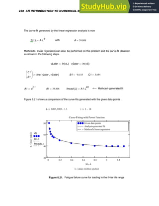
![6.10.2. Temperature Response of an Object Placed in a Hot Stream of Air
The following data pertains to the temperatures of a solid steel sphere suspended in a hot stream
of air measured at several instants of time [ 17 ]. It is required to curve-fit the data with a suitable
function.
t= Time (secs) T=Temp (deg C) t=Time(Secs) T=Temp (deg C)
0.0 14 500 51
100 28 600 54
200 37.5 700 55
300 44 800 57.8
400 48 900 59.1
The given data is put in as follows and plotted in Figure 6.22.
n 10
:= t1 0
:= t2 100
:= t3 200
:= t4 300
:= t5 400
:= t6 500
:= t7 600
:=
T1 14
:= T2 28
:= T3 37.5
:= T4 44
:= T5 48
:= T6 51
:= T7 54
:=
t8 700
:= t9 800
:= t10 900
:= T8 55
:= T9 57.8
:= T10 59.1
:=
i 1 10
..
:=
0 200 400 600 800
0
20
40
60
Given data points
Given data points
Ti
ti
Figure 6.22. Given temperature versus time data
A glance at the plot of Figure 6.22 suggests that a function of the following form would provide a
reasonable fit to the given data
f t
( ) A B e
t
−
τ
⋅
+
=
where f(t) is a linear combination of functions in which A and B are constants to be determined
on a least squares basis. From the data plot, it appears that the temperature profile attains
steady state in approximately 1200 seconds, which , when equated to four time constants, will
yield a time constant, τ, of 300 seconds. Thus, the coefficient of t in the exponential term can
be selected as (-1/300).
Chapter 6: Curve-Fitting 239](https://image.slidesharecdn.com/anintroductiontonumericalmethodsusingmathcadmathcadrelease14-230805170449-0ea94cc2/85/AN-INTRODUCTION-TO-NUMERICAL-METHODS-USING-MATHCAD-Mathcad-Release-14-249-320.jpg)
![In this case, the matrix equation to be solved is
[M] {C} = {A}
in which {M] and {A} contain the functions f1 t
( ) 1
:= f2 t
( ) e
1
−
300
t
⋅
:=
and
M
1
n
i
f1 ti
( )2
∑
=
1
n
i
f1 ti
( ) f2 ti
( )
⋅
( )
∑
=
1
n
i
f1 ti
( ) f2 ti
( )
⋅
( )
∑
=
1
n
i
f2 ti
( )2
∑
=
⎡
⎢
⎢
⎢
⎢
⎢
⎢
⎣
⎤
⎥
⎥
⎥
⎥
⎥
⎥
⎦
:= , C
C1
C2
⎛
⎜
⎝
⎞
⎟
⎠
= , A
1
n
i
f1 ti
( ) Ti
⋅
( )
∑
=
1
n
i
f2 ti
( ) Ti
⋅
( )
∑
=
⎡
⎢
⎢
⎢
⎢
⎢
⎢
⎣
⎤
⎥
⎥
⎥
⎥
⎥
⎥
⎦
:=
In the above, note that n = 10 and m =2, and the unknown constants are C1 and C2 which are
determined below using lsolve.
C lsolve M A
,
( )
:= A C1
:= B C2
:=
C
60.477
45.967
−
⎛
⎜
⎝
⎞
⎟
⎠
=
The function fitting the given data , then, is
f t
( ) A B e
1
−
300
t
⋅
⋅
+
:=
which is shown in Figure 6.23 .
f 0
( ) 14.511
= f 200
( ) 36.877
= f 800
( ) 57.283
= f 900
( ) 58.189
=
Mathcad's function linfit can also be used to evaluate the undetermined coefficients A and B in
the regression function employed which is a linear combination of the functions selected for the
curve-fit. This can be done as shown in the following steps.
vt t
:= vT T
:= F t
( )
1
e
1
−
300
t
⋅
⎛
⎜
⎜
⎜
⎝
⎞
⎟
⎟
⎟
⎠
:= S linfit vt vT
, F
,
( )
:=
240 AN INTRODUCTION TO NUMERICAL METHODS USING MATHCAD](https://image.slidesharecdn.com/anintroductiontonumericalmethodsusingmathcadmathcadrelease14-230805170449-0ea94cc2/85/AN-INTRODUCTION-TO-NUMERICAL-METHODS-USING-MATHCAD-Mathcad-Release-14-250-320.jpg)
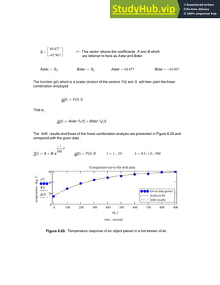
![6.10.3. The Effect of Operating Temperature on the Strength of a Mechanical
Element
When a mechanical element is subjected to reversed stresses at temperatures below room
temperature, there is a strong possibility of the occurrence of brittle fracture . On the other
hand, when the operating temperatures are higher than room temperature, the yield strength
of the material drops off very rapidly with increase in temperature, and yielding can take place
. The temperature-corrected value of tensile strength, then, to be used in design calculations
is obtained by multiplying the tensile strength at room temperature by a factor K d which is
a function of the temperature of the operating environment.
The following data was collected from tests done on carbon and alloy steels and shows the
effect of operating temperature on tensile strength [ 18 ]. An appropriate curve-fit to the
given data is sought.
Temp., deg F. K d Temp.,deg F. Kd
0 0.975 600 0.963
100 1.008 700 0.927
200 1.020 800 0.872
300 1.024 900 0.797
400 1.018 1000 0.698
500 0.995 1100 0.567
The given data points, which are plotted in Figure 6.24 below, are put in as follows.
n 12
:= T1 0
:= T2 100
:= T3 200
:= T4 300
:= T5 400
:= T6 500
:=
T7 600
:= T8 700
:= T9 800
:= T10 900
:= T11 1000
:= T12 1100
:=
Kd1 0.975
:= Kd2 1.008
:= Kd3 1.020
:= Kd4 1.024
:= Kd5 1.018
:= Kd6 0.995
:=
Kd7 0.963
:= Kd8 0.927
:= Kd9 0.872
:= Kd10 0.797
:= Kd11 0.698
:= Kd12 0.567
:=
242 AN INTRODUCTION TO NUMERICAL METHODS USING MATHCAD](https://image.slidesharecdn.com/anintroductiontonumericalmethodsusingmathcadmathcadrelease14-230805170449-0ea94cc2/85/AN-INTRODUCTION-TO-NUMERICAL-METHODS-USING-MATHCAD-Mathcad-Release-14-252-320.jpg)
![0 200 400 600 800 1000
0.5
1
Given data points
Given data points
Given data points
Temperature, deg. F
Factor
Kd
Kdi
Ti
i 1 12
..
:=
Figure 6.24. Given Kd versus temperature data
We will fit the given data with a second-order polynomial of the following form.
Kd(T) = f(T) = C1 + C2 T + C3T 2
Here, n = 12 and m = 2 and the matrix equation to be solved is:
[M]{C} = {A},
where [M] is a known 3x3 matrix and {A} is a known column vector as shown below. The
column vector {C} , which involves the undetermined coefficients, is
C
C1
C2
C3
⎛
⎜
⎜
⎜
⎝
⎞
⎟
⎟
⎟
⎠
=
The [M] and {A} matrices are
Chapter 6: Curve-Fitting 243](https://image.slidesharecdn.com/anintroductiontonumericalmethodsusingmathcadmathcadrelease14-230805170449-0ea94cc2/85/AN-INTRODUCTION-TO-NUMERICAL-METHODS-USING-MATHCAD-Mathcad-Release-14-253-320.jpg)
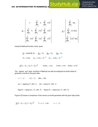
![0 200 400 600 800 1000
0.4
0.6
0.8
1
1.2
Given data points
Analysis-generated function
Mathcad regress
Mathcad loess
Given data points
Analysis-generated function
Mathcad regress
Mathcad loess
Curve-fits generated
Temperature, deg F
Multiplying
factor
Kd
vKdi
f T
( )
freg T
( )
floess T
( )
vTi T
,
Figure 6.25. Effect of operating temperature on the strength of a mechanical element
6.10.4. Drop-Testing of Packaged Articles
An interesting parameter that often warrants investigation is the height from which a package can
be dropped before it suffers any accountable damage, which can be assessed from the maximum
acceleration imparted to the package at the end of the drop [ 20 ]. This is a question that arises
when packages must be properly cushioned before shipment to another location. The maximum
acceleration to gravity ratio, a , has been found to be a function of the ratio, h , of twice the
distance dropped to the static deflection of the package.
The following a versus h data is provided , using which a reasonable curve-fit is to be
generated .
h a h a
________________________
1 1.4 9 3.25
2 1.8 10 3.3
3 2 11 3.55
4 2.25 12 3.65
5 2.65 13 3.75
6 2.8 14 3.85
7 2.9 15 4.2
8 3.01 16 4.3
_______________________________
Chapter 6: Curve-Fitting 245](https://image.slidesharecdn.com/anintroductiontonumericalmethodsusingmathcadmathcadrelease14-230805170449-0ea94cc2/85/AN-INTRODUCTION-TO-NUMERICAL-METHODS-USING-MATHCAD-Mathcad-Release-14-255-320.jpg)
![These data points are plotted in Figure 6.26.
n 16
:= i 1 2
, 16
..
:= h1 1
:= hi 1
+ hi 1
+
:=
a1 1.4
:= a2 1.8
:= a3 2.
:= a4 2.25
:= a5 2.65
:= a6 2.8
:= a7 2.9
:= a8 3.01
:=
a9 3.25
:= a10 3.3
:= a11 3.55
:= a12 3.65
:= a13 3.75
:= a14 3.85
:= a15 4.2
:= a16 4.3
:=
We will generate a curve-fit of the form:
a = f(h) = C1 + C2 h + C3 h 2 + C 4 h 3
Here, n = 16 and m = 3 and the matrix equation to be solved is:
[M]{C} = {A},
0 2 4 6 8 10 12 14 16
1
2
3
4
5
Given data points
Given data points
Given data points
(2h/ static deflection ) ratio
(max
acceleration/
gravity)
ratio
ai
hi
Figure 6.26. Given acceleration ratio versus height ratio data
246 AN INTRODUCTION TO NUMERICAL METHODS USING MATHCAD](https://image.slidesharecdn.com/anintroductiontonumericalmethodsusingmathcadmathcadrelease14-230805170449-0ea94cc2/85/AN-INTRODUCTION-TO-NUMERICAL-METHODS-USING-MATHCAD-Mathcad-Release-14-256-320.jpg)
![where [M] is a known 4x4 matrix and {A} is a known column vector as shown below. The
column vector {C} , which involves the undetermined coefficients, is
C
C1
C2
C3
C4
⎛
⎜
⎜
⎜
⎜
⎜
⎝
⎞
⎟
⎟
⎟
⎟
⎟
⎠
=
M
n
1
n
i
hi
∑
=
1
n
i
hi
( )2
∑
=
1
n
i
hi
( )3
∑
=
1
n
i
hi
∑
=
1
n
i
hi
( )2
∑
=
1
n
i
hi
( )3
∑
=
1
n
i
hi
( )4
∑
=
1
n
i
hi
( )2
∑
=
1
n
i
hi
( )3
∑
=
1
n
i
hi
( )4
∑
=
1
n
i
hi
( )5
∑
=
1
n
i
hi
( )3
∑
=
1
n
i
hi
( )4
∑
=
1
n
i
hi
( )5
∑
=
1
n
i
hi
( )6
∑
=
⎡
⎢
⎢
⎢
⎢
⎢
⎢
⎢
⎢
⎢
⎢
⎢
⎢
⎢
⎢
⎢
⎣
⎤
⎥
⎥
⎥
⎥
⎥
⎥
⎥
⎥
⎥
⎥
⎥
⎥
⎥
⎥
⎥
⎦
:=
A
1
n
i
ai
∑
=
1
n
i
hi ai
⋅
( )
∑
=
1
n
i
hi
( )2
ai
⋅
⎡
⎣
⎤
⎦
∑
=
1
n
i
hi
( )3
ai
⋅
⎡
⎣
⎤
⎦
∑
=
⎡
⎢
⎢
⎢
⎢
⎢
⎢
⎢
⎢
⎢
⎢
⎢
⎢
⎢
⎢
⎢
⎣
⎤
⎥
⎥
⎥
⎥
⎥
⎥
⎥
⎥
⎥
⎥
⎥
⎥
⎥
⎥
⎥
⎦
:=
C lsolve M A
,
( )
:= C
0.997
0.433
0.029
−
9.472 10
4
−
×
⎛
⎜
⎜
⎜
⎜
⎝
⎞
⎟
⎟
⎟
⎟
⎠
= C1 C1
:= C2 C2
:= C3 C3
:= C4 C4
:=
C1 0.997
= C2 0.433
= C3 0.029
−
= C4 9.472 10
4
−
×
=
f h
( ) C1 C2 h
⋅
+ C3 h
2
⋅
+ C4 h
3
⋅
+
:= f 15
( ) 4.114
= f 9
( ) 3.219
=
The Mathcad regress and loess functions also can be utilized as shown below to generate
curve-fits to the given data.
Chapter 6: Curve-Fitting 247](https://image.slidesharecdn.com/anintroductiontonumericalmethodsusingmathcadmathcadrelease14-230805170449-0ea94cc2/85/AN-INTRODUCTION-TO-NUMERICAL-METHODS-USING-MATHCAD-Mathcad-Release-14-257-320.jpg)
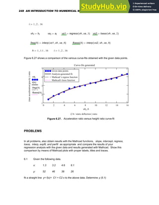


![Strain,e, ( %) Stress,S, (Kpsi)
10 63
20 63.6
40 62
60 60
80 58
100 56
120 52
140 48
150 47
Using an approximating polynomial of the form
S C1 C2 e
⋅
+ C3 e
2
⋅
+
=
obtain a least squares fit to the given data. Determine S(105%)
6. 16. The following data relating the distance traveled by an object to time was obtained from a
test in an experimental test track . The distance traveled, S, is in meters and the time , t, is in
seconds.
Time, t (secs) 0.1 0.5 1.5 3.0
Distance, S (m) 0.26 1.56 7.41 30.90
Generate a curve-fit of the form S(t) = A + B t + C t 2. Compute S for t= 2 seconds.
6.17. The pressure drag , D P, on an object can be reduced in comparison with the total
drag , DT, by streamlining it , that is, making its length, L, in the direction of flow larger with
respect to its maximum thickness or diameter, D . [ 17 ] . Obtain an appropriate curve-fit to
the following data which is provided to demonstrate the effect of streamlining on the pressure
drag of a body of symmetrical airfoil cross section.
L
D
1 2 3 4 5 6 7 8 9 10 11
( )
=
DP
DT
1.25 0.65 0.42 0.25 0.20 0.10 0.08 0.06 0.04 0.02 0.01
( )
=
Determine D P / DT for L / D = 5.5
6.18. The following data , in which the time, t, is given in seconds provides the
252 AN INTRODUCTION TO NUMERICAL METHODS USING MATHCAD](https://image.slidesharecdn.com/anintroductiontonumericalmethodsusingmathcadmathcadrelease14-230805170449-0ea94cc2/85/AN-INTRODUCTION-TO-NUMERICAL-METHODS-USING-MATHCAD-Mathcad-Release-14-262-320.jpg)
![response c ( t ) of a control system to a step input.
t 0 0.75 1.50 2 3 4 5 6
( )
:=
c t
( ) 0 1.30 1.40 1.10 0.85 1.02 1.01 1.009
( )
:=
Obtain a least-squares fit of the form.
c(t)= A+ B e -t sin (2.828 t ) + C e -t cos ( 2.828 t )
and determine c at t = 3.5 seconds.
6.19. The Brinell hardness number, Bhn , for steel [ 18 ] is given as a function of the
tempering temperature, T, in the following table
T, deg F. 400 600 800 1000 1200
Bhn 540 500 445 375 310
Obtain an appropriate curve-fit to the given data and determine the Brinell hardness
number for T = 850 deg F.
6.20. The average strain rate used in obtaining stress/ strain data for a material
specimen is about 0.001 in / (in-sec ). However, when the strain rate, SR, is
increased, as it happens, under conditions of impact loading, the strength of the
material also increases. [ 18 ] The following data shows the influence of the
increase in strain rate on the yield strength, SYLD, of a steel specimen
SR 10
6
−
10
5
−
10
4
−
10
2
−
1 10
2
10
3
( )
= in/(in-sec)
SYLD 30 28 30 37 45 65 78
( )
= kpsi
Obtain an appropriate least-squares fit to the given data and determine SYLD
corresponding to an SR of 50.
6.21. The endurance limit of a steel specimen is, typically, a function of the condition
of its surface [ 19 ]. For an unnotched, ground specimen in reversed bending,
the endurance limit, S end , is related to its tensile strength, S ult , as given in the
following table of data.
Sult 60 80 100 120 140 160 180 200 220
( )
= kpsi
Send 25 35 45 55 65 72 80 85 90
( )
= kpsi
Chapter 6: Curve-Fitting 253](https://image.slidesharecdn.com/anintroductiontonumericalmethodsusingmathcadmathcadrelease14-230805170449-0ea94cc2/85/AN-INTRODUCTION-TO-NUMERICAL-METHODS-USING-MATHCAD-Mathcad-Release-14-263-320.jpg)
![Obtain a reasonable curve-fit to the given data. Determine S end corresponding to S ult = 135
kpsi .
6.22. Expected voice levels required for speech communication with various back-
ground noise levels and separations between the speaker and the listener [ 10 ]
are given in the following table of data .
Obtain appropriate curve-fits to the given data in the form of separate curves for
(a) Peak shouting (b) Shouting (c) Very loud voice (d) Raised voice and (e)
Normal voice.
Determine the voice levels required in the following situations.
(1) Speaker listener distance = 2.5 m , background noise level = 68 dBA
(2) Speaker listener distance = 4.5 m , background noise level = 86 dBA
(3) Speaker listener distance = 8.5 m , background noise level = 45 dBA
(4) Speaker listener distance = 6.5 m , background noise level = 65 dBA
BACKGROUND NOISE LEVELS (dBA)
Speaker
/listener
distance
( m )
Normal
Voice
Raised
Voice
Very
Loud
Voice
Shouting Peak
Shouting
0.25
0.5
1.0
2
3
4
5
6
7
8
9
9.5
⎛
⎜
⎜
⎜
⎜
⎜
⎜
⎜
⎜
⎜
⎜
⎜
⎜
⎜
⎜
⎜
⎝
⎞
⎟
⎟
⎟
⎟
⎟
⎟
⎟
⎟
⎟
⎟
⎟
⎟
⎟
⎟
⎟
⎠
90
80
72
63
57
54.5
52
50
49.5
49
48
47.5
⎛
⎜
⎜
⎜
⎜
⎜
⎜
⎜
⎜
⎜
⎜
⎜
⎜
⎜
⎜
⎜
⎝
⎞
⎟
⎟
⎟
⎟
⎟
⎟
⎟
⎟
⎟
⎟
⎟
⎟
⎟
⎟
⎟
⎠
62
60
57
56.5
55
54
53.5
52.5
⎛
⎜
⎜
⎜
⎜
⎜
⎜
⎜
⎜
⎜
⎜
⎜
⎜
⎜
⎜
⎜
⎜
⎝
⎞
⎟
⎟
⎟
⎟
⎟
⎟
⎟
⎟
⎟
⎟
⎟
⎟
⎟
⎟
⎟
⎟
⎠
95
88
78
72
68
66
64
62.5
61.5
60
58
57.5
⎛
⎜
⎜
⎜
⎜
⎜
⎜
⎜
⎜
⎜
⎜
⎜
⎜
⎜
⎜
⎜
⎝
⎞
⎟
⎟
⎟
⎟
⎟
⎟
⎟
⎟
⎟
⎟
⎟
⎟
⎟
⎟
⎟
⎠
100
92
84
77
74
72
68
67.5
66
65
64.5
64
⎛
⎜
⎜
⎜
⎜
⎜
⎜
⎜
⎜
⎜
⎜
⎜
⎜
⎜
⎜
⎜
⎝
⎞
⎟
⎟
⎟
⎟
⎟
⎟
⎟
⎟
⎟
⎟
⎟
⎟
⎟
⎟
⎟
⎠
118
112
103
96
92.5
90
88
86.5
86
85
84.5
84
⎛
⎜
⎜
⎜
⎜
⎜
⎜
⎜
⎜
⎜
⎜
⎜
⎜
⎜
⎜
⎜
⎝
⎞
⎟
⎟
⎟
⎟
⎟
⎟
⎟
⎟
⎟
⎟
⎟
⎟
⎟
⎟
⎟
⎠
254 AN INTRODUCTION TO NUMERICAL METHODS USING MATHCAD](https://image.slidesharecdn.com/anintroductiontonumericalmethodsusingmathcadmathcadrelease14-230805170449-0ea94cc2/85/AN-INTRODUCTION-TO-NUMERICAL-METHODS-USING-MATHCAD-Mathcad-Release-14-264-320.jpg)


![ffourprime
1
∆x
4
1.853 4 1.723
⋅
− 6 1.456
⋅
+ 4 1.212
⋅
− 0.703
+
( )
⋅
:= ffourprime 0.448
−
=
7.3. INTERPOLATING POLYNOMIAL METHOD
In the interpolating polynomial method, an interpolating polynomial passing through given
data points is determined by any of the methods discussed in Chapter 5. Then, the
polynomial generated can be differentiated as is done in traditional calculus. If the polynomial
derived , for instance, is
f x
( ) a0 a1 x
⋅
+ a2 x
2
⋅
+ a3 x
3
⋅
+ ............
+ an x
n
⋅
+
= (7.10)
then, its derivative can be obtained as
x
f x
( )
d
d
a1 2 a2
⋅ x
⋅
+ 3 a3
⋅ x
2
⋅
+ ..............
+ n an
⋅ x
n 1
−
⋅
+
= (7.11)
Example 7.2
Given the following data :
x 2 3 4 5 6
y 0.80354 1.23591 1.62312 1.89765 1.96789
Use the Method of Undetermined Coefficients to fit an interpolating polynomial to the given
data and estimate: yprime(4.5), yprime(2.7), ydblprime(4.5) and ydblprime(2.7).
Since 5 data points are given, we can generate a 4 th order polynomial.
Let y(x) = f(x)= a + bx + cx2 + dx3 + e x4
Substituting the given values of (x,y) in the assumed polynomial above yields the following
matrix equation:
[M]{A}= {V}
where
Chapter 7: Numerical Differentiation 259](https://image.slidesharecdn.com/anintroductiontonumericalmethodsusingmathcadmathcadrelease14-230805170449-0ea94cc2/85/AN-INTRODUCTION-TO-NUMERICAL-METHODS-USING-MATHCAD-Mathcad-Release-14-269-320.jpg)

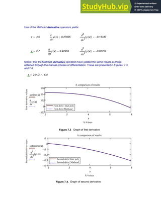
![Determine the velocity and acceleration of the train as functions of time. Estimate the
velocity and acceleration of the train at t = 32 seconds
We first use the method of undetermined coefficients to fit an interpolating polynomial to
the given data. Since six data points are given, a fifth order polynomial of the following
form will be generated.
s(t) = f(t)= a + bt + ct2 + dt3 + e t4 + f t 5
Substituting the given values of (t,s) in the assumed polynomial above yields the following
matrix equation:
[M]{A} = {V}
where
V
0
75
175
360
480
600
⎛
⎜
⎜
⎜
⎜
⎜
⎜
⎜
⎝
⎞
⎟
⎟
⎟
⎟
⎟
⎟
⎟
⎠
:=
M
1
1
1
1
1
1
0
10
20
30
35
40
0
2
10
2
20
2
30
2
35
2
40
2
0
3
10
3
20
3
30
3
35
3
40
3
0
4
10
4
20
4
30
4
35
4
40
4
0
5
10
5
20
5
30
5
35
5
40
5
⎛
⎜
⎜
⎜
⎜
⎜
⎜
⎜
⎜
⎜
⎜
⎝
⎞
⎟
⎟
⎟
⎟
⎟
⎟
⎟
⎟
⎟
⎟
⎠
:=
Using the Mathcad function lsolve, the unknown coefficients in the column vector {A} can be found
A lsolve M V
,
( )
:=
A
0
9.41429
0.36131
−
0.01667
7.7381 10
5
−
×
4.52381
− 10
6
−
×
⎛
⎜
⎜
⎜
⎜
⎜
⎜
⎜
⎜
⎝
⎞
⎟
⎟
⎟
⎟
⎟
⎟
⎟
⎟
⎠
=
Chapter 7: Numerical Differentiation 263](https://image.slidesharecdn.com/anintroductiontonumericalmethodsusingmathcadmathcadrelease14-230805170449-0ea94cc2/85/AN-INTRODUCTION-TO-NUMERICAL-METHODS-USING-MATHCAD-Mathcad-Release-14-273-320.jpg)

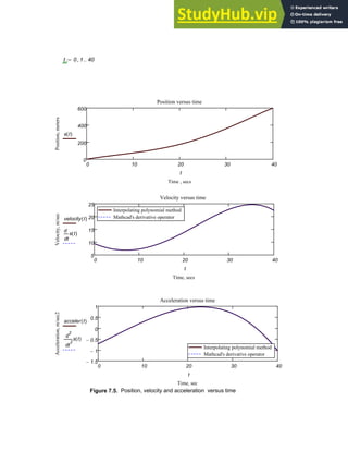
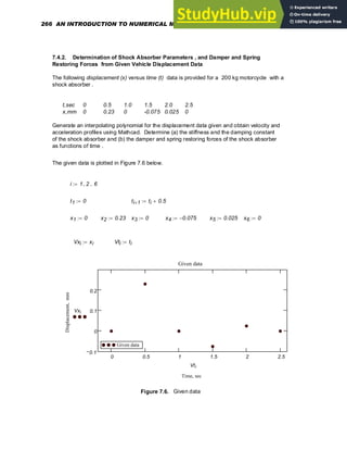
![As done in the preceding problem, we first use the method of undetermined coefficients to fit an
interpolating polynomial to the given data. Since six data points are prescribed , a fifth order
polynomial of the following form can be generated.
x(t) = f(t)= a + bt + ct2 + dt3 + e t4 + f t 5
Substituting the given values of (t,x) in the assumed polynomial above yields the following matrix
equation:
[M]{A}= {V}
where
M
1
1
1
1
1
1
0
0.5
1
1.5
2
2.5
0
2
0.5
2
1
2
1.5
2
2
2
2.5
2
0
3
0.5
3
1
3
1.5
3
2
3
2.5
3
0
4
0.5
4
1
4
1.5
4
2
4
2.5
4
0
5
0.5
5
1
5
1.5
5
2
5
2.5
5
⎛
⎜
⎜
⎜
⎜
⎜
⎜
⎜
⎜
⎜
⎜
⎝
⎞
⎟
⎟
⎟
⎟
⎟
⎟
⎟
⎟
⎟
⎟
⎠
:= V
0
0.23
0
0.075
−
0.025
0
⎛
⎜
⎜
⎜
⎜
⎜
⎜
⎜
⎝
⎞
⎟
⎟
⎟
⎟
⎟
⎟
⎟
⎠
:=
A lsolve M V
,
( )
:= A
0
1.7375
3.69917
−
2.65167
0.76333
−
0.07333
⎛
⎜
⎜
⎜
⎜
⎜
⎜
⎜
⎝
⎞
⎟
⎟
⎟
⎟
⎟
⎟
⎟
⎠
=
The coefficients a, b, c, d. e and f of the assumed polynomial are
a A1
:= a 0
= c A3
:= c 3.69917
−
= d A4
:= d 2.65167
=
b A2
:= b 1.737
= e A5
:= e 0.76333
−
= f A6
:= f 0.073
=
Chapter 7: Numerical Differentiation 267](https://image.slidesharecdn.com/anintroductiontonumericalmethodsusingmathcadmathcadrelease14-230805170449-0ea94cc2/85/AN-INTRODUCTION-TO-NUMERICAL-METHODS-USING-MATHCAD-Mathcad-Release-14-277-320.jpg)
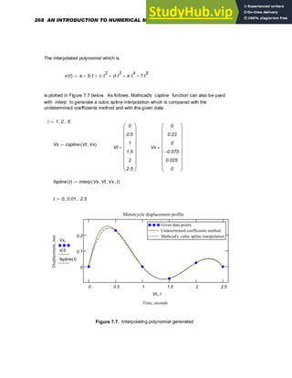
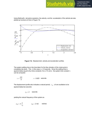
![As shown below , the damping, c , and stiffness, k , furnished by the shock absorber
can be computed using the pertinent formulas available in textbooks in Vibrations and
Controls [ 6, 9, 14, 16, 20, 21].
Damping factor x undamped natural frequency = 1/ system time constant :
ζωn
1
τ
:= ζωn 1.6
=
Since ζωn and ωd are known , the damping factor ζ can be calculated.
ωd ωn 1 ζ
2
−
⋅
=
ωd 2
π
τd
⋅
:= ωd 3.142
= rad/sec ζ
ζωn
2
ωd
2
ζωn
2
+
:= ζ 0.454
=
The undamped natural frequency of the system along with the stiffness and damping coefficients
of the shock absorber can now be computed using
ωn
ζωn
ζ
:= ωn 3.526
= rad/sec
The stiffness and damping coefficients of the shock absorber can now be determined.
m 200
:= kg
k m ωn
2
⋅
:= k 2.486 10
3
×
= N/m
c 2 m
⋅ ωn
⋅ ζ
⋅
:= c 640
= N-sec/ m
The shock absorber spring and damper restoring forces which can now be calculated as functions
of time using
270 AN INTRODUCTION TO NUMERICAL METHODS USING MATHCAD](https://image.slidesharecdn.com/anintroductiontonumericalmethodsusingmathcadmathcadrelease14-230805170449-0ea94cc2/85/AN-INTRODUCTION-TO-NUMERICAL-METHODS-USING-MATHCAD-Mathcad-Release-14-280-320.jpg)
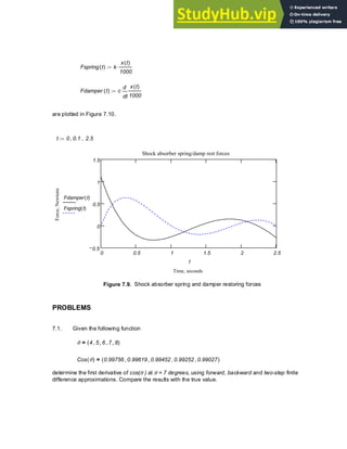


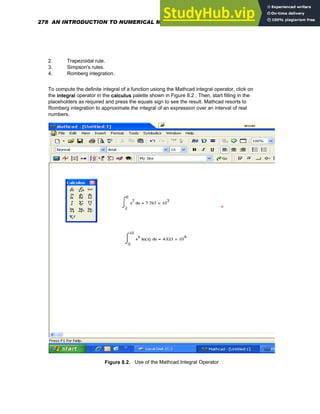
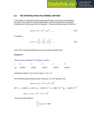
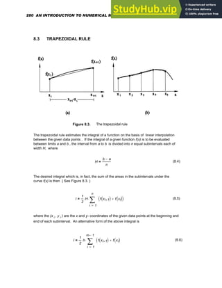
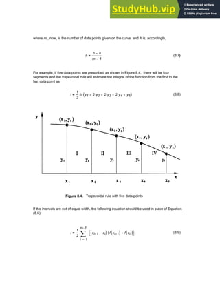

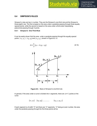
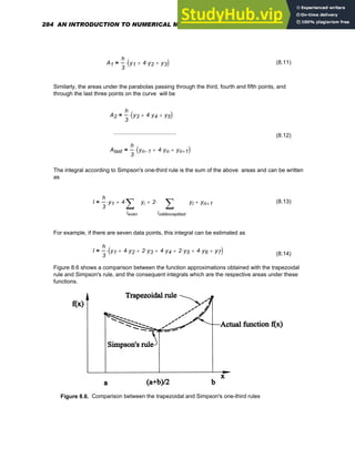

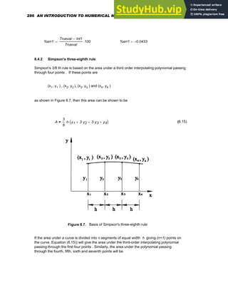

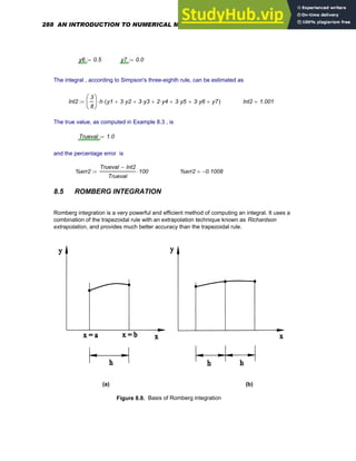
![The procedure for computing the integral of f(x) over a prescribed range of x= a to x= b by
the Romberg method is as follows.
1. For a range of integration from x =a to x= b, a shown in Figure 8.8 (a) ,obtain
the first trapezoidal estimate I 0,1 of the integral of the given function f(x) by the trapezoidal
rule as
(8.19)
I0 1
,
1
2
h
⋅ f a
( )
( f b
( )
+
[ ]
⋅
=
where h b a
−
= (8.20)
2. Divide the given range into two segments as shown in Figure 8.8 (b) and obtain
the second trapezoidal estimate I 1,1 as
I1 1
,
h
2
y1 2 y2
⋅
+ y3
+
( )
⋅
= (8.21)
where
h
b a
−
2
=
y1 f a
( )
= <--Value of function at the beginning of the range of
integration
(8.22)
y2 f a h
+
( )
= <--Value of function at the middle of the range of
integration
y3 f a 2 h
⋅
+
( )
= <--Value of function at the end of the range of
integration
3 Now divide the given range further into four segments and obtain the third
trapezoidal estimate I 2,1 with h = one-half of the previous h = (b-a)/4 .
4. Obtain a fourth trapezoidal estimate I 3,1with eight segments and h = (b-a)/8
5. Obtain a fifth trapezoidal estimate I 4,1 with sixteen segments and h = (b-a)/16
6. Using the Richardson extrapolation formula which is
Chapter 8: Numerical Integration 289](https://image.slidesharecdn.com/anintroductiontonumericalmethodsusingmathcadmathcadrelease14-230805170449-0ea94cc2/85/AN-INTRODUCTION-TO-NUMERICAL-METHODS-USING-MATHCAD-Mathcad-Release-14-299-320.jpg)
![Ii j
, Ii j 1
−
,
1
4
j 1
−
1
−
Ii j 1
−
, Ii 1
− j 1
−
,
−
( )
⋅
+
= (8.23)
compute the other unknown components of the matrix [I] , namely ,
I1 2
, I2 2
, I2 3
, I3 2
, I3 3
, I3 4
,
I4 2
, I4 3
, I4 4
, I4 5
, ............
and fill in the Romberg table which is shown in Table 8.1. Keep filling in the table
until the integral values converge , i.e,
I3 3
, I3 2
,
= or I4 3
, I4 2
,
= or I4 4
, I4 3
,
=
whichever occurs earlier.
TABLE 8.1
The Romberg table
R
I0 1
,
I1 1
,
I2 1
,
I3 1
,
I4 1
,
I5 1
,
I1 2
,
I2 2
,
I3 2
,
I4 2
,
I5 2
,
I2 3
,
I3 3
,
I4 3
,
I5 3
,
I3 4
,
I4 4
,
I5 4
,
I4 5
,
I5 5
, I5 6
,
⎛
⎜
⎜
⎜
⎜
⎜
⎜
⎜
⎜
⎜
⎜
⎝
⎞
⎟
⎟
⎟
⎟
⎟
⎟
⎟
⎟
⎟
⎟
⎠
:=
The procedure of this method should be clear from the examples that follow.
290 AN INTRODUCTION TO NUMERICAL METHODS USING MATHCAD](https://image.slidesharecdn.com/anintroductiontonumericalmethodsusingmathcadmathcadrelease14-230805170449-0ea94cc2/85/AN-INTRODUCTION-TO-NUMERICAL-METHODS-USING-MATHCAD-Mathcad-Release-14-300-320.jpg)

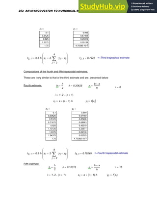
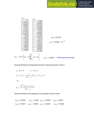
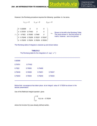


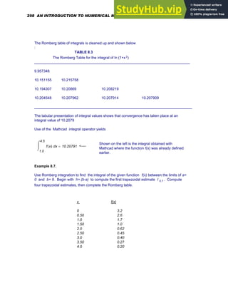
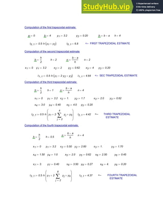
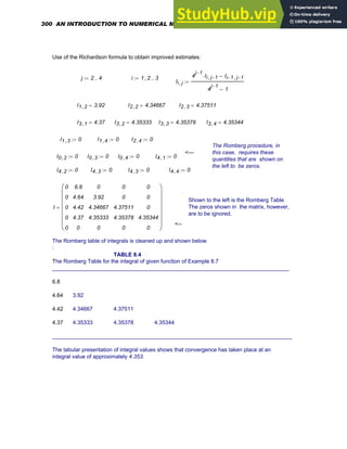
![8.6 APPLICATIONS IN NUMERICAL INTEGRATION
Applications of numerical integration can be encountered in situations dealing with location of
centroids, determination of moments of inertia of cross sectional shapes and computation of
periods of oscillations in nonlinear vibration problems. Some examples are dealt with below.
8.6.1 Centroid of a Rod Bent into the Shape of a Parabola
The length of an element dL of a rod bent into the shape of the parabola shown in Figure 8.8
can be expressed in terms of the differentials dx and dy as [ 8 ]
dL dx
2
dy
2
+
= or 1
y
x
d
d
⎛
⎜
⎝
⎞
⎟
⎠
2
+ dy
⋅ (8.24)
Since x 2 y
2
⋅
= ,
y
x
d
d
4 y
×
= and dL 1 16 y
2
⋅
+ dy
⋅
=
y x
( )
x
2
:= x 0 0.001
, 0.5
..
:=
0 0.1 0.2 0.3 0.4
0
0.2
0.4
bent shape of rod
bent shape of rod
Rod of parabolic shape: x = 2 y .y
x , meters
y,
meters
y x
( )
x
Figure 8.8. Rod bent into a parabolic shape
The length of the rod , then, can be written as
L L
1
⌠
⎮
⎮
⌡
d
= or L
0
0.5
y
1 16 y
2
⋅
+
⌠
⎮
⌡
d
:= L 0.739
= meters
Chapter 8: Numerical Integration 301](https://image.slidesharecdn.com/anintroductiontonumericalmethodsusingmathcadmathcadrelease14-230805170449-0ea94cc2/85/AN-INTRODUCTION-TO-NUMERICAL-METHODS-USING-MATHCAD-Mathcad-Release-14-311-320.jpg)
![The location of the centroid ( x CG , y CG ) can then be calculated using
xCG
L
x
⌠
⎮
⎮
⌡
d
L
= yCG
L
y
⌠
⎮
⎮
⌡
d
L
=
or,
xCG
1
L 0
0.5
y
2 y
2
⋅ 1 16 y
2
⋅
+
⋅
⌠
⎮
⌡
d
⋅
:= yCG
1
L 0
0.5
y
y 1 16 y
2
⋅
+
⋅
⌠
⎮
⌡
d
⋅
:=
giving
xCG 0.205
= m yCG 0.287
= m
8.6.2. Moment of Inertia of a Beam of Semi-Elliptic Cross Section
For the semi-elliptic beam cross section shown in Figure 8.9 , its moments of inertia about
the x and y axes can be calculated using [ 8 ]
Ixx A
y
2
⌠
⎮
⎮
⌡
d
= Iyy A
x
2
⌠
⎮
⎮
⌡
d
= (8.25)
where
dA 2 x
⋅ dy
⋅
= with x y
( ) 1
y
2
b
2
− a
⋅
= and a 4
:= in b 2
:= in
dA y dx
⋅
= with y x
( ) 1
x
2
a
2
− b
⋅
:= x 4
− 3.99
−
, 4.
..
:=
4 2 0 2 4
0
2
Semi-elliptic cross section
y x
( )
x
The moments of inertia , I xx and I yy,
can now be computed as follows,using
Equations (8.25)
Ixx 2
a
b
⋅
0
b
y
y
2
b
2
y
2
−
⋅
⌠
⎮
⌡
d
⋅
:=
Figure 8.9. Beam cross section
Iyy
b
a a
−
a
x
x
2
a
2
x
2
−
⋅
⌠
⎮
⌡
d
⋅
:= giving Ixx 12.566
= in 4 and Iyy 50.266
= in 4
302 AN INTRODUCTION TO NUMERICAL METHODS USING MATHCAD](https://image.slidesharecdn.com/anintroductiontonumericalmethodsusingmathcadmathcadrelease14-230805170449-0ea94cc2/85/AN-INTRODUCTION-TO-NUMERICAL-METHODS-USING-MATHCAD-Mathcad-Release-14-312-320.jpg)
![8.6.3. Launch of a Projectile
A projectile is launched with an initial vertical velocity vy init from a height y 0 above the ground.
Neglecting air resistance, the relationship between its vertical velocity v y at any time t and the
height y above the ground that it attains on the way up is given by [ 8 ]
vy vyinit
2
2 G
⋅ y0 y
−
( )
⋅
+
= (8.26)
where G is the acceleration due to gravity ( 32.2 ft/ sec 2 or 9.81 m/ sec 2 ) . Equating the
above quantity to dy/dt , and then integrating with respect to time from 0 to t seconds, the
following expression can be derived for the time t taken by the projectile to attain the height
y above the ground
t
y0
y
y
1
vyinit
2
2 G
⋅ y0 y
−
( )
⋅
+
⌠
⎮
⎮
⎮
⌡
d
=
(8.27)
The time taken to reach the maximum height , y max , is then the above integral with
y max as the upper limit of integration , where
ymax
vyinit
2
2 G
⋅
y0
+
=
(8.28)
For an initial velocity of 55 ft/ sec at an angle of 65 degrees from a height of 3.5 ft above ground, the
time taken to attain the maximum height is calculated below using Equations (8.27) and (8.28).
vinit 55
:= ft/sec θ 65 deg
⋅
:= sin θ
( ) 0.906
= G 32.2
:= ft/ sec 2
vyinit vinit sin θ
( )
⋅
:= vyinit 49.847
= ft/sec y0 3.5
:= ft
ymax
vyinit
2
2 G
⋅
y0
+
:= ymax 42.083
= ft
tmaxheight
y0
ymax
y
1
vyinit
2
2 G
⋅ y0 y
−
( )
⋅
+
⌠
⎮
⎮
⎮
⌡
d
:= tmaxheight 1.548
= sec
Chapter 8: Numerical Integration 303](https://image.slidesharecdn.com/anintroductiontonumericalmethodsusingmathcadmathcadrelease14-230805170449-0ea94cc2/85/AN-INTRODUCTION-TO-NUMERICAL-METHODS-USING-MATHCAD-Mathcad-Release-14-313-320.jpg)
![8.6.4. Large Oscillations of a Simple Pendulum
A simple pendulum, which is a mass attached to one end of a light rigid rod, is shown in Figure
8.10.
Figure 8.10. Vibration of a simple pendulum
The large-amplitude motion of this pendulum is governed by the following nonlinear differential
equation [ 6,9,16,20 ].
2
t
θ t
( )
d
d
2 G
L
sin θ t
( )
( )
⋅
+ 0
= (8.29)
where L is the length of the rod and G is the acceleration due to gravity . However, if the
amplitudes of vibration are considered small, the above differential equation assumes
its linear form
2
t
θ t
( )
d
d
2 G
L
θ t
( )
⋅
+ 0
= (8.30)
and the motion, then, has a natural period
τlinear 2 π
⋅
L
G
⋅
:= seconds (8.31)
For the nonlinear problem , it can be shown that the period of one oscillation, which is now a
function of the amplitude of vibration , is given by the integral
304 AN INTRODUCTION TO NUMERICAL METHODS USING MATHCAD](https://image.slidesharecdn.com/anintroductiontonumericalmethodsusingmathcadmathcadrelease14-230805170449-0ea94cc2/85/AN-INTRODUCTION-TO-NUMERICAL-METHODS-USING-MATHCAD-Mathcad-Release-14-314-320.jpg)
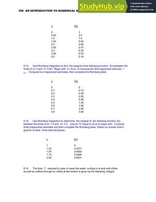
![T
H1
H2
h
A
Q k h
0.5
⋅
−
⌠
⎮
⎮
⎮
⌡
d
=
where H1 and H2 are the initial and final heights of the water surface above the base of the
tank , A is the cross sectional area of the tank , Q is the inflow rate, and k is a constant
that depends on the coefficient of discharge and the area of the orifice. Determine how long
it will take for the water level to fall 10 ft in a tank 50 ft long by 30 ft wide with vertical sides,
when water enters the tank at the rate of 6 cu. ft / sec and the initial level of the water
surface in the tank is 16 ft above the bottom. Take k to be 3.
8.16. The motion of bodies moving with moderate speed in fluids such as
water or air is resisted by a damping force that is proportional to the square of the speed. In
order to estimate the resonant amplitude of the motion, the equivalent linear viscous
damping, C eq , is needed which is found by equating the energy dissipated by the viscous
damping in one cycle to that of the nonviscous damping [ 20 ]. The equivalent viscous
damping, in this case , can be shown to be
Ceq
2 a
⋅ ω
⋅ X
⋅
π 0
π
θ
sin θ
( )
3
⌠
⎮
⌡
d
⋅
=
where a is a proportionality constant that depends on the body geometry and the
properties of the fluid medium , ω is the frequency of excitation and X is the
amplitude of the resulting vibration. Determine C eq if a = 0.85 N-sec 2 / m , ω = 550
rads/ sec and X = 16 mm.
8.17. The moment of inertia of a sphere of radius R about a diametral axis is given by
the integral [ 8 ]
Idia
1
2
ρ
⋅ π
⋅
R
−
R
x
R
(
2
x
2
−
⎡
⎣ ⎤
⎦
2
⌠
⎮
⎮
⌡
d
⋅
=
where ρ is the mass density of the material of the sphere. Estimate I dia for a 1 m
diameter sphere made of steel with ρ = 7.8 Mg / m 3
8.18. The shear stress distribution in a beam cross section subjected to a shear force
V is given by [ 18 ]
Chapter 8: Numerical Integration 309](https://image.slidesharecdn.com/anintroductiontonumericalmethodsusingmathcadmathcadrelease14-230805170449-0ea94cc2/85/AN-INTRODUCTION-TO-NUMERICAL-METHODS-USING-MATHCAD-Mathcad-Release-14-319-320.jpg)


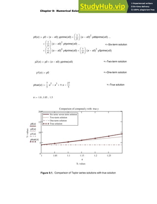
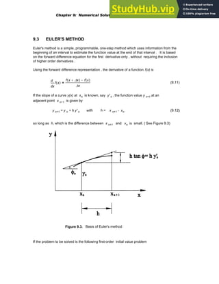
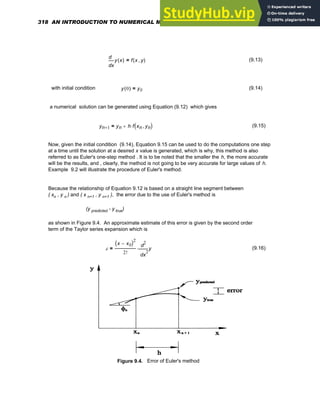

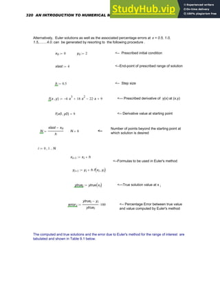

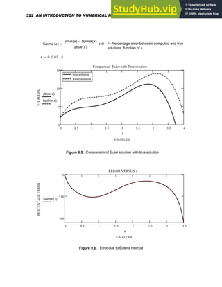
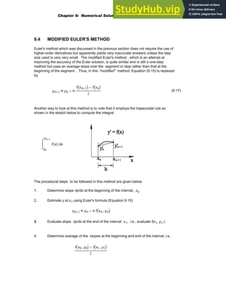
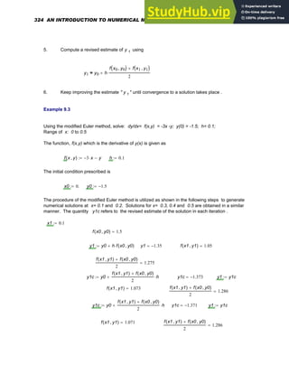

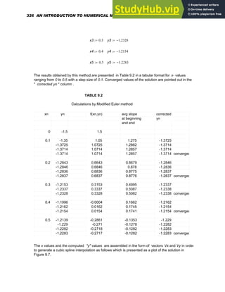
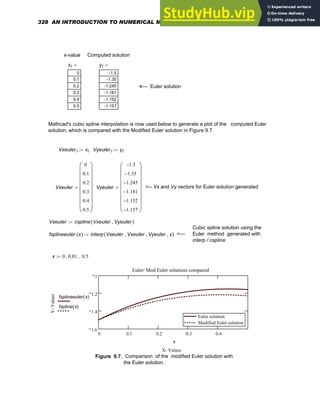
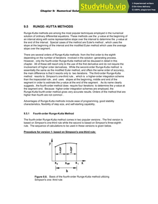


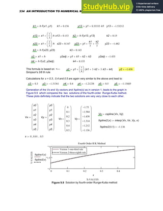

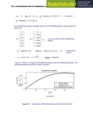
![Example 9.7.
Using the Runge-Kutta fourth-order method, obtain a solution to
dx/dt = f(x,y,t) = xy2 + t; dy/dt= g(x,y,t) = ty + x2
for t = 0 to t= 0.5 seconds. The initial conditions are given as: x(0)= -1; y (0) = 1
Use a time increment of h = 0.1 second.
Note that both x and y are functions of the independent variable " t".
Thus, in this case,
dx/dt = f(x,y,t ) = xy2 + t ,
and dy/dt = g(x,y,t) = ty + x2
Version 1 of the Runge-Kutta Method which utilizes Simpson's one-third rule, will then resort
to the following sequential equations to compute x and y at t1, where t1 = t0 + h., and h is
the increment or step size
k1 = h f(x0, y0, t0) ; m1= h g(x0,y0, t0) ;
tmp = t0 + 0.5 h ; xmp= x0+ 0.5 k1; ymp= y0+0.5 m1
k2= h f(xmp, ymp, tmp) ; m2 = h g( xmp, ymp, tmp )
xmp* = x0 + 0.5 k2 ; ymp* = y0+ 0.5 m2
k3 = h f ( xmp*, ymp*, tmp ) ; m3 = h g ( xmp*, ymp*, tmp )
x1 = x0 + k3 ; y1 = y0 + m3 ; t1 = t0 + h
k4 = h f ( x1, y1, t1 ) ; m4 = h g ( x1, y1, t1 )
x1= x0 + (1/6) [ k1 +2 k2 + 2 k3 + k4 ] ; y1 = y0 + (1/6 ) [ m1 + 2 m2 + 2 m3 + m4 ]
In order to compute the solution (x1,y1) at t1, we start with known values x0, y0 and t0 as
shown above. Similarly, to compute the solution (x2, y2) at t2, the above procedure needs to
be repeated with ( x1, y1 , t1) replacing (x0, y0,t0) and (x2,y2,t2) replacing (x1,y1,t1).
Define the functions f(x,y,t) and g(x,y,t), the step size and the initial conditions:.
342 AN INTRODUCTION TO NUMERICAL METHODS USING MATHCAD](https://image.slidesharecdn.com/anintroductiontonumericalmethodsusingmathcadmathcadrelease14-230805170449-0ea94cc2/85/AN-INTRODUCTION-TO-NUMERICAL-METHODS-USING-MATHCAD-Mathcad-Release-14-352-320.jpg)


![t x y
Note: The first column contains the
t-values, the second column contains
the x-values, and the third contains the
y- values
Value
0
5 10
3
−
×
0.03
0.155
0.374387
0.5
1
−
1.005025
−
1.030966
−
1.190367
−
1.800212
−
3.026613
−
1
1.005038
1.031388
1.197505
1.741152
2.524711
⎛
⎜
⎜
⎜
⎜
⎜
⎜
⎜
⎜
⎝
⎞
⎟
⎟
⎟
⎟
⎟
⎟
⎟
⎟
⎠
=
<---
It is noted that the Runge-Kutta- Version 1 solution agrees reasonably well with the
Mathcad solutions.
9.7 SOLUTION OF HIGHER-ORDER ORDINARY DIFFERENTIAL
EQUATIONS
In many areas of engineering and physics, the solution of higher-order differential equations is
often required. Examples can be encountered in vibration engineering, control systems
engineering , electrical circuit analysis etc.
The general form of a second-order differential equation is
d2y/dx2 = f ( x, y, dy/dx ) (9.27)
A more special form often encountered in vibrations, control systems, and electrical circuit
analysis is
a d2y/dx2 + b dy/dx + c y = q(x) (9.28)
with initial conditions y(0) and dy/dx(0) specified.
Although any of the methods discussed in sections 9.2-9.5 can certainly be used to obtain
solutions to Equation 9.28, it must first be converted to a system of first-order differential
equations as follows.
dy/dx = z = f ( x,y, z)
dz/dx = [q(x) - b z - c y] / a = g (x,y, z )
(9.29)
Chapter 9: Numerical Solution of Ordinary Differential Equations 349](https://image.slidesharecdn.com/anintroductiontonumericalmethodsusingmathcadmathcadrelease14-230805170449-0ea94cc2/85/AN-INTRODUCTION-TO-NUMERICAL-METHODS-USING-MATHCAD-Mathcad-Release-14-359-320.jpg)
![with the initial conditions now becoming y(0) and z(0) . Thus, if a solution to the second-order
differential equation, which is now represented by the two first-order equations of Equations
9.29 , is to be generated by Version 1 of the fourth-order Runge-Kutta method, the
calculations shown in the following procedure must be resorted to.
k1 = h f (y0, z0, x0) ; m1= h g (y0,z0, x0) ;
xmp = x0 + 0.5 h ; ymp= y0+ 0.5 k1; zmp= z0+0.5 m1
k2= h f (ymp, zmp, xmp) ; m2 = h g ( ymp, zmp, xmp )
ymp* = y0 + 0.5 k2 ; zmp* = z0+ 0.5 m2
k3 = h f ( ymp*, zmp*, xmp ) ; m3 = h g ( ymp*, zmp*, xmp )
y1 = y0 + k3 ; z1 = z0 + m3 ; x1 = x0 + h
k4 = h f ( y1, z1, x1 ) ; m4 = h g ( y1, z1, x1 )
y1= y0 + (1/6) [ k1 +2 k2 + 2 k3 + k4 ] ; z1 = z0 + (1/6 ) [ m1 + 2 m2 + 2 m3 + m4 ]
(9.30)
where h is the increment or step size. Note that in order to generate the solution
(y1, z1), we started with known values ( x0, y0, z0 ). Similarly, to obtain ( y2, z2) , the above
procedure must be repeated with (x1,y1,z1) replacing ( x0, y0,z0) and (x2, y2,z2) replacing
(x1,y1,z1).
Example 9.8
Using the Runge-Kutta fourth-order
method, obtain a solution to
m d2y/dt2 +c dy/dt + k y = F(t) ;
m= 1kg, c= 3 N-sec/m, k = 9 N/m , F(t)= 9 N.
for t = 0 to t= 3 seconds. The initial conditions
are given as: y(0)=0; dy/dt (0) = 0 .
Use a time increment of 0.5 seconds.
350 AN INTRODUCTION TO NUMERICAL METHODS USING MATHCAD](https://image.slidesharecdn.com/anintroductiontonumericalmethodsusingmathcadmathcadrelease14-230805170449-0ea94cc2/85/AN-INTRODUCTION-TO-NUMERICAL-METHODS-USING-MATHCAD-Mathcad-Release-14-360-320.jpg)
![The above differential equation represents the equation of motion of a linear
spring-mass-damper system subjected to a step forcing function as shown in the above figure.
As mentioned earlier , application of the fourth order Runge- Kutta Method to the solution of a
second-order differential equation is quite similar to that of a first order differential equation ,
except that the following two first-order equations must now be considered.
dy/dt = z ;
and m dz/dt + c z +k y = F(t)
Note that, now, both y and z are functions of the independent variable " t".
Thus, in this case,
dy/dt = f( y,z, t ) = z ,
and dz/dt = g(y,z,t) =[F(t) - ( k y + c z)] /m
Version 1 of the R-K procedure will then resort to the following equations to compute y and z at
t1:
k1 = h f(y0, z0, t0) ; m1= h g(y0,z0, t0) ;
tmp = t0 + 0.5 h ; ymp= y0+ 0.5 k1; zmp= z0+0.5 m1
k2= h f(ymp, zmp, tmp) ; m2 = h g( ymp, zmp, tmp )
ymp* = y0 + 0.5 k2 ; zmp* = z0+ 0.5 m2
k3 = h f ( ymp*, zmp*, tmp ) ; m3 = h g ( ymp*, zmp*, tmp )
y1 = y0 + k3 ; z1 = z0 + m3 ; t1 = t0 + h
k4 = h f ( y1, z1, t1 ) ; m4 = h g ( y1, z1, t1 )
y1= y0 + (1/6) [ k1 +2 k2 + 2 k3 + k4 ] ; z1 = z0 + (1/6 ) [ m1 + 2 m2 + 2 m3 + m4 ]
Chapter 9: Numerical Solution of Ordinary Differential Equations 351](https://image.slidesharecdn.com/anintroductiontonumericalmethodsusingmathcadmathcadrelease14-230805170449-0ea94cc2/85/AN-INTRODUCTION-TO-NUMERICAL-METHODS-USING-MATHCAD-Mathcad-Release-14-361-320.jpg)
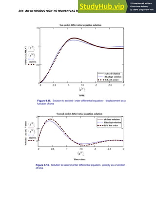

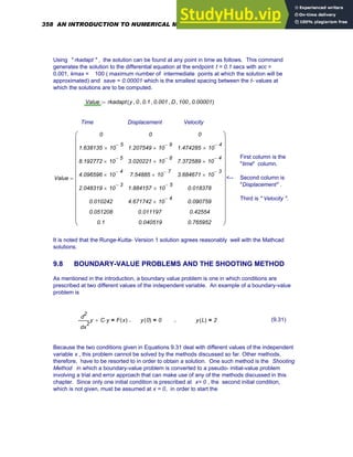
![solution process. Upon completion of the solution process, a check must be made to
determine if the condition prescribed at the point x = L is satisfied or not. If not, a second
guess must be made and the procedure redone. If the second guess still does not satisfy the
prescribed end condition, a third guess has to be estimated. This can be accomplished by
noting the difference between the given and the computed conditions at x = L and resorting to
a linear interpolation process that utilizes the results of the first two trials. This iteration
process must be repeated until the prescribed end condition is , in fact, satisfied. In this
method, it is important for the analyst to be skillful at estimating the unprescribed initial
condition properly at the starting point in order to maintain efficiency and avoid divergence.
Because the method is analogous to aiming properly and shooting at a given object, it has
been appropriately labelled as the shooting method. When higher-order differential equations
must be solved involving several boundary conditions, this method has proven to be quite
uncouth and laborious and, thus, inefficient.
Although any of the methods discussed in this chapter can be employed in the solution of a
boundary-value problem by the shooting method. the following example will illustrate its
application with Mathcad's Rkadapt and rkadapt functions.
Example 9.9
Solve: d2y/ dx2 = M/EI = (30 x - 1.5 x^2)/ EI , where EI = 121,500 kips-ft 2
The boundary conditions prescribed are:
x = 0, y = 0 and x= 20, y =0
This differential equation represents the relationship between the bending moment M and
the deflection "y" at a distance "x" along the span from the left hand end of a 20 foot long
simply supported beam loaded with a uniformly distributed load of 3 kips/ ft. as shown in
Figure 9.17. The slope and deflection at any point " x " can be obtained by solving the above
differential equation.
Consider the two equations:
dy/dx = z ; and
(9.32)
dz/dx = M/EI = (30 x - 1.5 x^2 )/ EI
Note that, now, both y and z are functions of the dependent variable " x". Thus, in this
case,
dy/dx = f ( x, y, z ) = z ,
(9.33)
and dz/dx = g( x, y, z ) =[30 x - 1.5 x ^2 ] / EI
As said earlier, the shooting method is a trial- and- error method used in the solution of
boundary-value problems. Although two boundary conditions are prescribed here, there is
only one initial condition ( x= 0, y = 0 ) provided to begin the solution process. The initial
Chapter 9: Numerical Solution of Ordinary Differential Equations 359](https://image.slidesharecdn.com/anintroductiontonumericalmethodsusingmathcadmathcadrelease14-230805170449-0ea94cc2/85/AN-INTRODUCTION-TO-NUMERICAL-METHODS-USING-MATHCAD-Mathcad-Release-14-369-320.jpg)
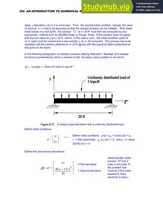
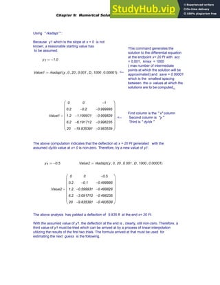
![New value of y1 to be tried = [second value of the first derivative y1 assumed times the
first deflection value at the end computed - first value of the first derivative y1 assumed
times the second deflection value at the end computed ] / [ first deflection value at the end
computed - the second deflection value at the end computed ] . That is,
y1
Value20 2
, Value14 1
,
⋅ Value10 2
, Value24 1
,
⋅
−
Value14 1
, Value24 1
,
−
:=
y1 8.23045
− 10
3
−
×
=
Then, the solution with the new guess is
Value3 rkadapt y 0
, 20
, 0.001
, D
, 1000
, 0.00001
,
( )
:=
which yields
Note the negligible
deflection
computed at the end with
the current assumed value
of the slope (derivative) at
x= 0
<----
Value3
0
0.2
1.2
6.2
20
0
1.645763
− 10
3
−
×
9.807565
− 10
3
−
×
0.042741
−
1.922074
− 10
15
−
×
8.230453
− 10
3
−
×
8.225547
− 10
3
−
×
8.059786
− 10
3
−
×
4.465547
− 10
3
−
×
8.230453 10
3
−
×
⎛
⎜
⎜
⎜
⎜
⎜
⎜
⎜
⎜
⎝
⎞
⎟
⎟
⎟
⎟
⎟
⎟
⎟
⎟
⎠
=
Now , using Rkadapt , the solution can be evaluated at 100 points between 0 and 20 with the
above initial slope value put in which led to the computation of the true displacement (y= 0) at the
end x= 20 Ft. The following commands will then generate the solution matrix [ Z ] which will
contain 3 columns- the "x" values, the corresponding "y" values and the "dy/dx " values.
Z Rkadapt y 0
, 20
, 100
, D
,
( )
:=
i 0 rows Z
( ) 1
−
..
:=
The results of the above Mathcad computation are plotted in Figures 9.18 and 9.19.
362 AN INTRODUCTION TO NUMERICAL METHODS USING MATHCAD](https://image.slidesharecdn.com/anintroductiontonumericalmethodsusingmathcadmathcadrelease14-230805170449-0ea94cc2/85/AN-INTRODUCTION-TO-NUMERICAL-METHODS-USING-MATHCAD-Mathcad-Release-14-372-320.jpg)
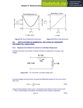
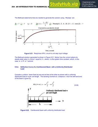
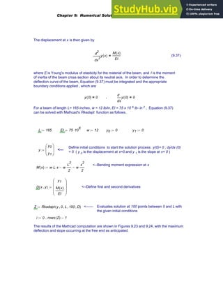
![0 100
0.2
0.1
0
Slope along beam span
Distance from left end
Slope
Z
2
〈 〉
( )i
Z
0
〈 〉
( )i
0 50 100 150
20
10
0
Deflection along beam span
Distance from left end, inches
Deflection
,
inches
Z
1
〈 〉
( )i
Z
0
〈 〉
( )i
Figure 9.23. Beam deflection curve Figure 9.24. Beam slope along span
9.9.3. Temperature Response of a Solid Steel Ball Placed in a Hot Stream Of Air
When a body which is initially at a uniform temperature T 0 is suddenly placed in a hot
fluid, the rate at which the temperature T(t) of the body changes with time is given by the
differential equation [ 17 ]
ρ c
⋅ Lc
⋅
t
T t
( )
d
d
⋅ h Tinf T t
( )
−
( )
⋅
= (9.38)
where ρ is the mass density of the body, c is its specific heat at constant pressure, T inf is
the temperature of the surrounding fluid, h is the average convection heat transfer coefficient,
and L c is the characteristic length. For a solid steel sphere of diameter 2 cm initially at 10 deg
C., and placed in a stream of hot air at temperature, T inf = 75 deg C. , with h =25 W/ m 2 . K,
we have
d 0.02
:= m ρ 7854
:= kg/ m 3
c 434
:= J/ kg . K h 25
:= W/ m 2 . K
Tinf 75
:= deg. K T0 10
:= deg. K V π
d
3
6
⋅
:= A π d
2
⋅
:=
Lc
V
A
:= Lc 3.333333 10
3
−
×
= m
and the Mathcad statements needed to generate the temperature response of the steel
ball to the hot stream of air are
366 AN INTRODUCTION TO NUMERICAL METHODS USING MATHCAD](https://image.slidesharecdn.com/anintroductiontonumericalmethodsusingmathcadmathcadrelease14-230805170449-0ea94cc2/85/AN-INTRODUCTION-TO-NUMERICAL-METHODS-USING-MATHCAD-Mathcad-Release-14-376-320.jpg)
![T0 10
:= D t T
,
( )
h
ρ c
⋅ Lc
⋅
Tinf T
−
( )
⋅
:= Z Rkadapt T 0.
, 2000
, 100
, D
,
( )
:=
i 0 rows Z
( ) 1
−
..
:=
0 500 1000 1500 2000
0
50
100
Temp response of steel ball
Time, seconds
Temperature,
deg.
C.
Z
1
〈 〉
( )i
Z
0
〈 〉
( )i
Figure 9.25. Temperature response of steel ball
The Mathcad solution generated, which is plotted in Figure 9.25 shows how the steel ball attains
its steady-state temperature of 75 deg C. in a time t equal to 4τ, where τ is the system time
constant which, in this case, is ρ c
⋅
Lc
h
⋅ = 454.5 seconds.
9.9.4. Nonlinear Vibration of a Simple Pendulum
The natural frequency of large oscillation of a simple pendulum, which is a mass attached
to one end of a light rigid rod, has been generated in Section 6 of Chapter 8 as a function
of the maximum amplitude of the pendulum. The nonlinear behavior of the pendulum is
governed by the differential equation [ 6, 9, 16, 20 ]
2
t
θ t
( )
d
d
2 G
L
sin θ t
( )
( )
⋅
+ 0
= (9.39)
where L is the length of the pendulum and G is the acceleration due to gravity .
Chapter 9: Numerical Solution of Ordinary Differential Equations 367](https://image.slidesharecdn.com/anintroductiontonumericalmethodsusingmathcadmathcadrelease14-230805170449-0ea94cc2/85/AN-INTRODUCTION-TO-NUMERICAL-METHODS-USING-MATHCAD-Mathcad-Release-14-377-320.jpg)
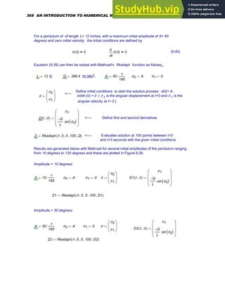
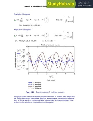
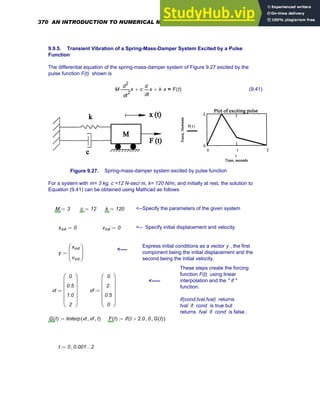
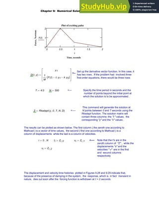
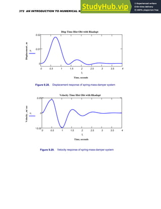
![9.9.6. Nonlinear Vibration of a Damped System with a Hardening Spring.
Consider the following nonlinear equation known as Duffing's equation [ 6, 16, 20, 21 ],
which is the differential equation of motion of a spring-mass-damper system with a
hardening spring
M
2
t
x
d
d
2
⋅ c
t
x
d
d
⋅
+ k x
⋅
+ μ x
3
⋅
+ F t
( )
= (9.42)
where the last term on the right hand side of the equation is due to the effect of the hardening
spring in which the spring stiffness increases as the load on it increases.
The term F(t) on the right hand side of the equation is the exciting force that the system
is subjected to. We will utilize Mathcad to obtain solutions to Equation (9.42) for m
= 1.2 kg, c= 0.6 N-sec/m , k= 1.2 N/ m and F(t) = (a) a step function and then (b) a
ramp function for values of μ ranging from 0.01 to 1.0. The results will then be compared with
those for μ =0
(a) Step input with μ =0, 0.01, 0.1, 1.0:
M 1.2
:= k 1.2
:= c 0.6
:=
xinit 0
:= vinit 0
:= <-- Specify initial displacement and velocity
Express initial conditions as a vector y , the first
component being the initial displacement and the
second being the initial velocity.
y
xinit
vinit
⎛
⎜
⎜
⎝
⎞
⎟
⎟
⎠
:= <----
F t
( ) Φ t
( )
:= This creates a unit step function (Φ(t)= unit
step or Heaviside function )
<----
0 0.2 0.4 0.6 0.8
0.998
0.999
1
1.001
Unit step input
Time, seconds
F(t),
Newtons
F t
( )
t
t 0 0.1
, 1.0
..
:=
Chapter 9: Numerical Solution of Ordinary Differential Equations 373](https://image.slidesharecdn.com/anintroductiontonumericalmethodsusingmathcadmathcadrelease14-230805170449-0ea94cc2/85/AN-INTRODUCTION-TO-NUMERICAL-METHODS-USING-MATHCAD-Mathcad-Release-14-383-320.jpg)
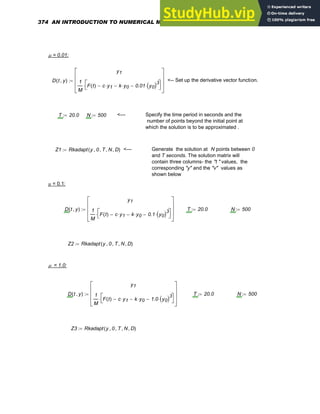
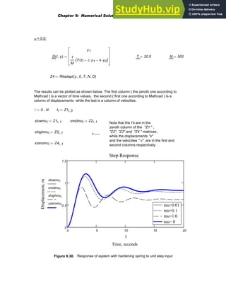
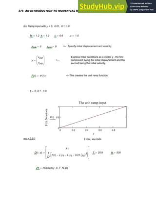
![0 5 10 15 20
0
5
10
15
20
mu= 0.01
mu= 0.1
mu= 1.0
mu = 0
mu= 0.01
mu= 0.1
mu= 1.0
mu = 0
Reponse to ramp input
Time, seconds
Displacement
,
m
xlowmui
xmidmui
xhighmui
xzeromui
ti
Figure 9.31. Response of system with hardening spring to a unit ramp input
9.9.7. Temperature Distribution in the Wall of a Pipe Carrying a Hot Fluid
The differential equation relating temperature in the wall of a metal pipe to radial distance is
[ 17 ]
r
2
r
T r
( )
d
d
2
⋅
t
T r
( )
d
d
+ 0
= (9.43)
where T(r) is the temperature in the pipe wall at a radial distance r from the pipe centerline. The
inner radius of the pipe is r i and the outer radius is r o . The temperature of the fluid inside the
pipe is T f while the temperature of the outer wall of the pipe is T o. Although two boundary
conditions are prescribed here, namely the temperatures at the inner and outer walls of the pipe,
there is only one initial condition available, that is , T(r i )= T f to begin the solution process.
The initial temperature gradient, namely, dT/dr , is not known. Thus, in order to resort to the
Shooting Method, this initial temperature gradient must be assumed so that the process of
generating a solution may be initiated. The solution T at ro must then be determined with these
initial values of T and dT/dr ( at r i ). If the solution obtained does not match up with the given
condition at r = r o , the assumed initial condition must be revised and a new solution T(r o )
determined. This process must be repeated until the solution obtained at r o agrees with the
prescribed condition . As discussed in Section 9.7, Equation (9.43) must first be converted to
the following two first- order differential equations before a solution can be obtained.
r
T
d
d
0
= ,
r
z
d
d
1
−
r
z
⋅
= (9.44)
378 AN INTRODUCTION TO NUMERICAL METHODS USING MATHCAD](https://image.slidesharecdn.com/anintroductiontonumericalmethodsusingmathcadmathcadrelease14-230805170449-0ea94cc2/85/AN-INTRODUCTION-TO-NUMERICAL-METHODS-USING-MATHCAD-Mathcad-Release-14-388-320.jpg)
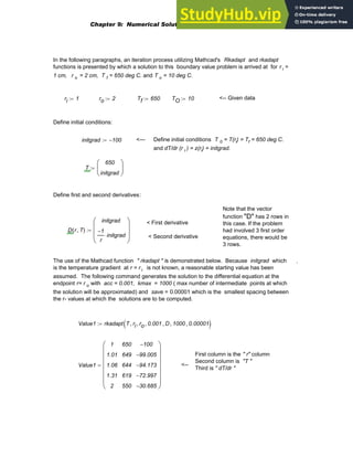
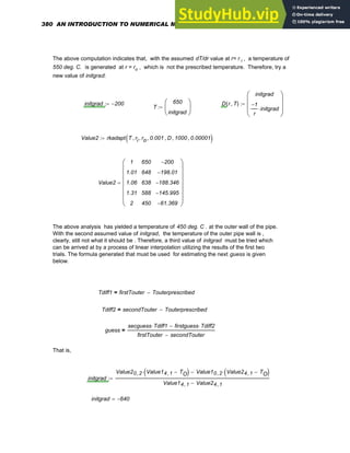
![Then, the solution with the new initgrad is
initgrad 640
−
= T
650
initgrad
⎛
⎜
⎝
⎞
⎟
⎠
:=
D r T
,
( )
initgrad
1
−
r
initgrad
⋅
⎛
⎜
⎜
⎝
⎞
⎟
⎟
⎠
:=
Value3 rkadapt T ri
, ro
, 0.001
, D
, 1000
, 0.00001
,
( )
:=
which yields
Note that the temperature
generated at the outer wall now
matches the prescribed
temperature (10 deg. C. ).
<----
Value3
1
1.01
1.06
1.31
2
650
643.6
611.6
451.6
10
640
−
633.632
−
602.708
−
467.183
−
196.382
−
⎛
⎜
⎜
⎜
⎜
⎜
⎜
⎝
⎞
⎟
⎟
⎟
⎟
⎟
⎟
⎠
=
Now , using Rkadapt , the solution can be evaluated at 100 points between r= 1 and r =
2 cm with the above initial dT/dr value put in which led to the computation of the true
temperature at the outer wall . The following commands will then generate the solution
matrix [ Z ] which will contain 3 columns- the "r" values, the corresponding "T" values
and the "dT/dr " values.
initgrad 640
−
= Z Rkadapt T ri
, ro
, 100
, D
,
( )
:=
D r T
,
( )
initgrad
1
−
r
initgrad
⋅
⎛
⎜
⎜
⎝
⎞
⎟
⎟
⎠
:=
i 0 rows Z
( ) 1
−
..
:=
The results of the above Mathcad computation are plotted in Figures 9.32 and 9.33.
Chapter 9: Numerical Solution of Ordinary Differential Equations 381](https://image.slidesharecdn.com/anintroductiontonumericalmethodsusingmathcadmathcadrelease14-230805170449-0ea94cc2/85/AN-INTRODUCTION-TO-NUMERICAL-METHODS-USING-MATHCAD-Mathcad-Release-14-391-320.jpg)
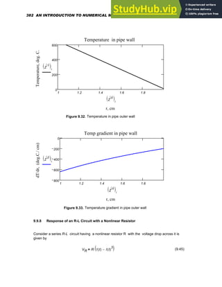
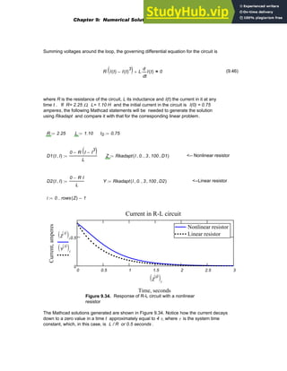
![9.9.9. The Effect of Damping on the Step Response of a Second-Order Control System
The general differential equation governing the behavior of a second-order control system
subjected to a unit step input is [ 14 ]
2
t
y t
( )
d
d
2
2 ζ
⋅ ωn
⋅
t
y t
( )
d
d
⎛
⎜
⎝
⎞
⎟
⎠
+ ωn
2
y t
( )
⋅
+ ωn
2
= (9.47)
where y(t) is the system response to the unit step input, ζ is the system damping ratio,
and ω n is the natural frequency of the undamped system. We want to investigate the dynamic
response of the system to different levels of damping obtained by varying ζ. If ωn = 5 rad/sec
and ζ is varied from 0.1 to1.4, the following Mathcad statements will be needed to generate the
rseponses .
ωn 5
:= y
0
0
⎛
⎜
⎝
⎞
⎟
⎠
:=
ζ1 0.1
:= D1 t y
,
( )
y1
ωn
2
2 ζ1
⋅ ωn
⋅ y1
⋅
− ωn
2
y0
⋅
−
⎛
⎜
⎜
⎝
⎞
⎟
⎟
⎠
:= Z1 Rkadapt y 0
, 10
, 1000
, D1
,
( )
:=
ζ2 0.2
:= D2 t y
,
( )
y1
ωn
2
2 ζ2
⋅ ωn
⋅ y1
⋅
− ωn
2
y0
⋅
−
⎛
⎜
⎜
⎝
⎞
⎟
⎟
⎠
:= Z2 Rkadapt y 0
, 10
, 1000
, D2
,
( )
:=
ζ3 0.6
:= D3 t y
,
( )
y1
ωn
2
2 ζ3
⋅ ωn
⋅ y1
⋅
− ωn
2
y0
⋅
−
⎛
⎜
⎜
⎝
⎞
⎟
⎟
⎠
:=
Z3 Rkadapt y 0
, 10
, 1000
, D3
,
( )
:=
ζ4 0.8
:= D4 t y
,
( )
y1
ωn
2
2 ζ4
⋅ ωn
⋅ y1
⋅
− ωn
2
y0
⋅
−
⎛
⎜
⎜
⎝
⎞
⎟
⎟
⎠
:= Z4 Rkadapt y 0
, 10
, 1000
, D4
,
( )
:=
384 AN INTRODUCTION TO NUMERICAL METHODS USING MATHCAD](https://image.slidesharecdn.com/anintroductiontonumericalmethodsusingmathcadmathcadrelease14-230805170449-0ea94cc2/85/AN-INTRODUCTION-TO-NUMERICAL-METHODS-USING-MATHCAD-Mathcad-Release-14-394-320.jpg)
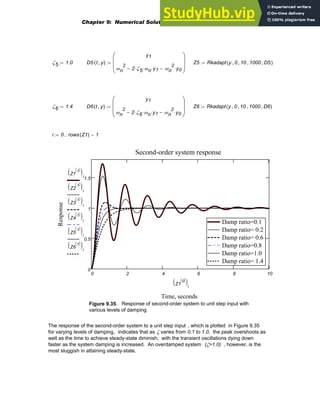


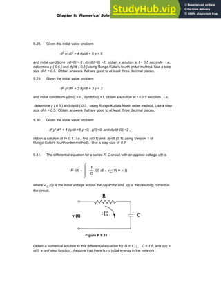
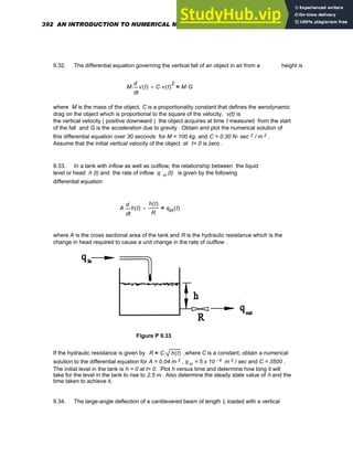


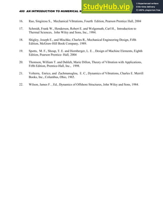
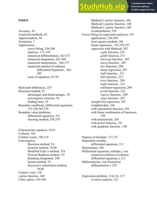
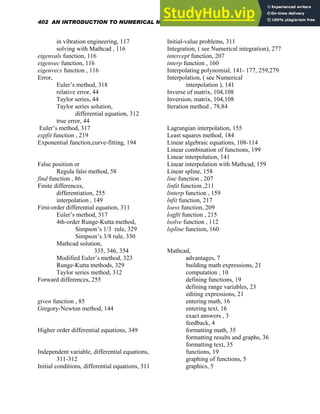


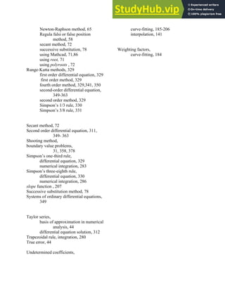

This document provides an introduction and overview to the textbook "An Introduction to Numerical Methods Using Mathcad" by Khyruddin Akbar Ansari. The textbook is designed as a guide for teaching numerical methods using Mathcad software. It covers topics such as root-finding, matrices, interpolation, curve-fitting, differentiation, integration, and solving differential equations. The author has many years of experience in engineering education and research.