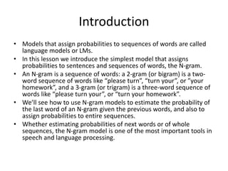
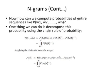
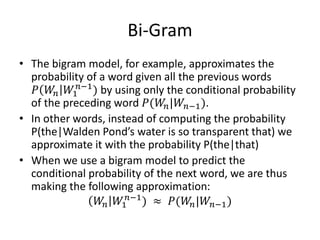
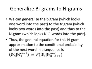
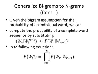
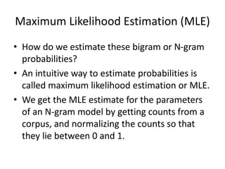
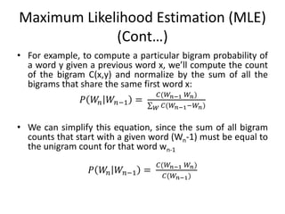
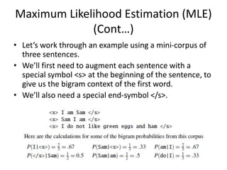
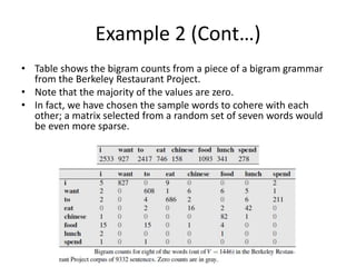
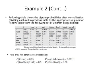
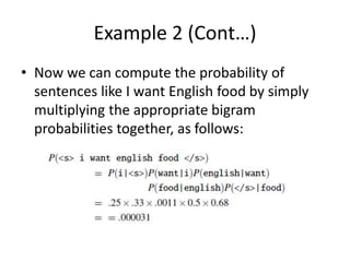
2. Introduction
• Models that assign probabilities to sequences of words are called
language models or LMs.
• In this lesson we introduce the simplest model that assigns
probabilities to sentences and sequences of words, the N-gram.
• An N-gram is a sequence of words: a 2-gram (or bigram) is a two-
word sequence of words like “please turn”, “turn your”, or ”your
homework”, and a 3-gram (or trigram) is a three-word sequence of
words like “please turn your”, or “turn your homework”.
• We’ll see how to use N-gram models to estimate the probability of
the last word of an N-gram given the previous words, and also to
assign probabilities to entire sequences.
• Whether estimating probabilities of next words or of whole
sequences, the N-gram model is one of the most important tools in
speech and language processing.
3. N-grams
• Let’s begin with the task of computing P(w|h),
the probability of a word w given some history
h.
• Suppose the history h is “its water is so
transparent that” and we want to know the
probability that the next word is the:
– P(the|its water is so transparent that):
4. N-grams (Cont…)
• One way to estimate this probability is from relative frequency counts:
take a very large corpus, count the number of times we see its water is so
transparent that, and count the number of times this is followed by the.
• This would be answering the question “Out of the times we saw the
history h, how many times was it followed by the word w”, as follows:
• With a large enough corpus, such as the web, we can compute these
counts and estimate the probability using above equation.
5. N-grams (Cont…)
• If we wanted to know the joint probability of
an entire sequence of words like its water is so
transparent, we could do it by asking “out of
all possible sequences of five words, how
many of them are its water is so transparent?”
• We would have to get the count of its water is
so transparent and divide by the sum of the
counts of all possible five word sequences.
• That seems rather a lot to estimate!
6. N-grams (Cont…)
• For this reason, we’ll need to introduce cleverer ways of
estimating the probability of a word w given a history h, or
the probability of an entire word sequence W.
• Let’s start with a little formalizing of notation.
• To represent the probability of a particular random variable
Xi taking on the value “the”, or P(Xi = “the”), we will use the
simplification P(the).
• We’ll represent a sequence of N words either as w1, …….,.
Wn or 𝑤1
𝑛
• For the joint probability of each word in a sequence having
a particular value P(X = w1, Y = w2, Z = w3, …..,W = wn)
we’ll use P(w1, w2, ……., wn).
7. N-grams (Cont…)
• Now how can we compute probabilities of entire
sequences like P(w1, w2, ……., wn)?
• One thing we can do is decompose this
probability using the chain rule of probability:
8. N-grams (Cont…)
• The chain rule shows the link between computing the joint probability of a
sequence and computing the conditional probability of a word given
previous words.
• Previous equation suggests that we could estimate the joint probability of
an entire sequence of words by multiplying together a number of
conditional probabilities.
• But using the chain rule doesn’t really seem to help us!
• We don’t know any way to compute the exact probability of a word given
a long sequence of preceding words, 𝑃 𝑊𝑛 𝑊1
𝑛−1
)
• As we said above, we can’t just estimate by counting the number of times
every word occurs following every long string, because language is
creative and any particular context might have never occurred before!
• The intuition of the N-gram model is that instead of computing the
probability of a word given its entire history, we can approximate the
history by just the last few words.
9. Bi-Gram
• The bigram model, for example, approximates the
probability of a word given all the previous words
𝑃 𝑊𝑛 𝑊1
𝑛−1
) by using only the conditional probability
of the preceding word 𝑃(𝑊𝑛|𝑊𝑛−1).
• In other words, instead of computing the probability
P(the|Walden Pond’s water is so transparent that) we
approximate it with the probability P(the|that)
• When we use a bigram model to predict the
conditional probability of the next word, we are thus
making the following approximation:
𝑊𝑛 𝑊1
𝑛−1
) ≈ 𝑃(𝑊𝑛|𝑊𝑛−1)
10. Markov Assumption
• The assumption that the probability of a
word depends only on the previous word is
called a Markov assumption.
• Markov models are the class of probabilistic
models that assume we can predict the
probability of some future unit without
looking too far into the past.
11. Generalize Bi-grams to N-grams
• We can generalize the bigram (which looks
one word into the past) to the trigram (which
looks two words into the past) and thus to the
N-gram (which looks N -1 words into the past).
• Thus, the general equation for this N-gram
approximation to the conditional probability
of the next word in a sequence is
𝑊𝑛 𝑊1
𝑛−1
) ≈ 𝑃(𝑊𝑛|𝑊𝑛−𝑁+1
𝑛−1
)
12. Generalize Bi-grams to N-grams
(Cont…)
• Given the bigram assumption for the
probability of an individual word, we can
• compute the probability of a complete word
sequence by substituting
𝑊𝑛 𝑊1
𝑛−1
) ≈ 𝑃(𝑊𝑛|𝑊𝑛−1)
• in to following equation:
𝑃 𝑊1
𝑛
=
𝑘=1
𝑛
𝑃(𝑊𝑘|𝑊𝑘−1)
13. Maximum Likelihood Estimation (MLE)
• How do we estimate these bigram or N-gram
probabilities?
• An intuitive way to estimate probabilities is
called maximum likelihood estimation or MLE.
• We get the MLE estimate for the parameters
of an N-gram model by getting counts from a
corpus, and normalizing the counts so that
they lie between 0 and 1.
14. Maximum Likelihood Estimation (MLE)
(Cont…)
• For example, to compute a particular bigram probability of
a word y given a previous word x, we’ll compute the count
of the bigram C(x,y) and normalize by the sum of all the
bigrams that share the same first word x:
𝑃 𝑊𝑛 𝑊𝑛−1 =
𝐶(𝑊𝑛−1 𝑊𝑛)
𝑊 𝐶(𝑊𝑛−1−𝑊𝑛)
• We can simplify this equation, since the sum of all bigram
counts that start with a given word (Wn-1) must be equal to
the unigram count for that word wn-1
𝑃 𝑊𝑛 𝑊𝑛−1 =
𝐶(𝑊𝑛−1 𝑊𝑛)
𝐶(𝑊𝑛−1)
15. Maximum Likelihood Estimation (MLE)
(Cont…)
• Let’s work through an example using a mini-corpus of
three sentences.
• We’ll first need to augment each sentence with a
special symbol <s> at the beginning of the sentence, to
give us the bigram context of the first word.
• We’ll also need a special end-symbol </s>.
16. Example 2
• Here are some text normalized sample user
queries extracted from Berkeley Restaurant
Project.
– can you tell me about any good cantonese restaurants
close by
– mid priced thai food is what i’m looking for tell me
about chez panisse
– can you give me a listing of the kinds of food that are
available
– i’m looking for a good place to eat breakfast
– when is caffe venezia open during the day
17. Example 2 (Cont…)
• Table shows the bigram counts from a piece of a bigram grammar
from the Berkeley Restaurant Project.
• Note that the majority of the values are zero.
• In fact, we have chosen the sample words to cohere with each
other; a matrix selected from a random set of seven words would
be even more sparse.
18. Example 2 (Cont…)
• Following table shows the bigram probabilities after normalization
(dividing each cell in previous table by the appropriate unigram for
its row, taken from the following set of unigram probabilities):
• Here are a few other useful probabilities:
19. Example 2 (Cont…)
• Now we can compute the probability of
sentences like I want English food by simply
multiplying the appropriate bigram
probabilities together, as follows: