NG3D902 - Basic Ray Optics Experiments - 2016

BASIC RAY OPTICS
EXPERIMENTS
Reflection, Snell’s Law, Total Internal
Reflection, Dispersion, Convex/Concave
Lenses and Lensmaker’s Equation
2016/2017
15060209
Christopher Francis
BSc (Hons) Electrical & Electronic
Engineering (Top up)
Lecturer: Dr Yongkang Gong
Lab Partner 1: Paul Farmilo
Lab Partner 2: Richard Hull

Abstract
This report discusses what happens when light waves reflect or pass from one transparent
medium boundary to another. The transition is bound by rules and is explained by
understanding the relationship between the Law of Reflection, Snell’s Law, Critical Angle,
Total Internal Reflection (TIR) and the Lensmaker’s Equation. The fundamentals of ray optics
were used to demonstrate the laws and their applications over six experiments. My role was to
lead the team, while Richard performed the procedures and Paul recorded the results. An initial
experiment explored the effects of light rays on different mirror surfaces to demonstrate
specular reflection, showing how the incident and reflected rays had the same angles with
respect to the normal in the same plane. A second experiment revealed the effects of refraction
in an acrylic trapezoid. Influential factors like the angle of approach, a change in light speed
and the index of refraction for transparent materials were reviewed. Snell’s Law was used to
calculate the index of refraction for acrylic and the results were verified with the accepted
norm. The third experiment was conducted on an acrylic trapezoid to identify the critical angle
at which refraction became non-existent and total internal reflection ensued. Snell’s Law was
used to show how critical angle was instrumental to the phenomena of TIR. A fourth
experiment studied the effects of dispersion, showing how a change in light wavelength has a
different index of refraction within the same material. The penultimate experiment revealed the
individual effects of refraction in both convex and concave lenses, which converged or
diverged respectively. By nesting the lenses, the light neither converged nor diverged, but
instead the incoming and outgoing rays became parallel. By spacing them apart, the distance
between the rays was varied. Finally, an experiment was conducted on a thin double concave
lens to demonstrate how the Lensmaker’s equation was used to calculate focal length. This
identified the relationship between focal length, the refractive index and the curved surfaces of
the lens. These experiments have important modern day applications such as fibre optic cables,
spectacles, cameras and many more.

Table of Contents
1. Reflection – Introduction ....................................................................................................5
2. Reflection – Equipment ......................................................................................................6
3. Reflection – Procedure........................................................................................................7
4. Reflection – Results ..........................................................................................................11
5. Reflection – Discussion ....................................................................................................13
6. Reflection – Conclusion....................................................................................................14
7. Snell’s Law – Introduction................................................................................................16
8. Snell’s Law – Equipment..................................................................................................17
9. Snell’s Law – Procedure ...................................................................................................18
10. Snell’s Law – Results........................................................................................................19
11. Snell’s Law – Discussion..................................................................................................21
12. Snell’s Law – Conclusion .................................................................................................22
13. Total Internal Reflection – Introduction ...........................................................................23
14. Total Internal Reflection – Equipment..............................................................................25
15. Total Internal Reflection – Procedure...............................................................................26
16. Total Internal Reflection – Results ...................................................................................28
17. Total Internal Reflection – Discussion..............................................................................30
18. Total Internal Reflection – Conclusion.............................................................................31
19. Dispersion – Introduction..................................................................................................32
20. Dispersion – Equipment....................................................................................................33
21. Dispersion – Procedure.....................................................................................................34
22. Dispersion – Results..........................................................................................................35
23. Dispersion – Discussion....................................................................................................37
24. Dispersion – Conclusion...................................................................................................38
25. Convex and Concave Lenses – Introduction.....................................................................39
26. Convex and Concave Lenses – Equipment.......................................................................40

27. Convex and Concave Lenses – Procedure ........................................................................41
28. Convex and Concave Lenses – Results.............................................................................43
29. Convex and Concave Lenses – Discussion.......................................................................44
30. Convex and Concave Lenses – Conclusion ......................................................................45
31. Lensmaker’s Equation – Introduction...............................................................................46
32. Lensmaker’s Equation – Equipment.................................................................................47
33. Lensmaker’s Equation – Procedure ..................................................................................48
34. Lensmaker’s Equation – Results.......................................................................................49
35. Lensmaker’s Equation – Discussion.................................................................................51
36. Lensmaker’s Equation – Conclusion ................................................................................52
37. References.........................................................................................................................53
38. Appendix 1 – Index of Refraction for Various Media ......................................................54
39. Appendix 2 – Experiment Photographs ............................................................................55

5 | P a g e
1. Reflection – Introduction
Reflection is a property of light that is bound by laws. Simply put, the law of reflection states
that the incident ray, the reflected ray, and the normal to the surface, all lie in the same plane.
This is known as the plane of incidence. Additionally, the angle of incidence is equal to the
angle of reflection with respect to the normal at the surface. Moreover, the incident and
reflected rays are on opposing sides of the normal (Hecht J. , 2008).
Figure 1 illustrates how a light beam that travels in a straight line, reflects from a mirrored
surface in one of two ways (Hecht E. , 2014):
a) Specular reflection – light incident upon a smooth mirror like surface, where all
Normals are parallel.
b) Diffuse reflection – light reflects from a rough surface, where the Normals are not
parallel.
Figure 1: (a) Specular reflection, and (b) diffuse reflection (Hecht E. , 2014).
The aim of the reflection experiment was to demonstrate an understanding of the law of
reflection within the context of specular reflection and to show how different mirror surfaces
have differing reflective effects. The basic nature of ray optics would be evaluated in terms of
focal length and the radius of curvature of a convex and concave mirror. This was achieved by
performing Experiment 3, which consisted of two parts:
 Part 1: Plane Mirror Experiment.
 Part 2: Cylindrical Mirror Experiment.

6 | P a g e
2. Reflection – Equipment
The following equipment was required to carry out the experiments:
 Light source – this multi-function desktop light source can be used in several modes,
including:
o Ray box mode – selects up to five white parallel rays.
o Ray box mode – selects three primary-colour rays.
 Ray optics kit – used in conjunction with the light source in ray box mode, the kit
comprises:
o Mirror (3-sided device with a convex, concave and a flat surface).
o Acrylic trapezoid (not required).
o Concave lens (not required).
o Convex lens (not required).
o Hollow lens (not required).
 Drawing compass – used to draw an arc or circle.
 Protractor – made from transparent plastic, this device is used for measuring angles in
degrees.
 Metric ruler – this device is used to measure the height, length or width of an object, or
the distance between two points.
 White paper – placed under the ray optics components, white paper helps to make the
light rays easier to view and trace.
 Pencil – used to trace the outline of the rays and the mirror.

7 | P a g e
3. Reflection – Procedure
3.1. Part 1 – Plane Mirror
3.1.1. Plug in the light source and switch it on, then place it on a sheet of white paper.
3.1.2. Select ray box mode by sliding the ray selector to single ray.
3.1.3. Turn off the laboratory lights to remove background lighting and place the mirror on
the white paper and position the flat surface at an appropriate angle to the light source,
so that the incident and reflected rays are clearly visible as shown in Figure 2:
Figure 2: Flat surface mirror arrangement.
3.1.4. Using a pencil, hold down and draw around the outside of the mirror.
3.1.5. Trace and label both the incoming incident ray and the outgoing reflected ray.
3.1.6. Indicate direction by using arrows on the drawing.
3.1.7. Now turn on the laboratory lights and remove the mirror and light source from the
paper.
3.1.8. Using a metric ruler, draw the normal to surface with a dotted line.
3.1.9. Using a protractor, measure and record the angles of incidence and reflection relative
to the normal. Store the results in Table 1.
3.1.10. Repeat steps 3 to 9, but reposition the light source to provide a different angle of
incidence. Obtain three sets of results with differing angles of incidence.
3.1.11. Next, set the light source so that the primary colour rays are visible.
3.1.12. Turn the sheet of white paper over and reposition the flat face of the mirror at an
appropriate angle to the light source. Ensure the primary colour incident and reflected
rays are clearly visible.

8 | P a g e
3.1.13. Use the pencil to mark the outline of the mirror and trace the primary colour incident
and reflected rays. Use arrows to indicate the incoming and outgoing direction as per
Figure 3:
Figure 3: Primary colour ray trace reflected from a flat mirror surface.
3.1.14. Record any law of reflection observations for evaluation later. Be sure to note the
time, date, team members and location of the experiment.
3.2. Part 2 – Cylindrical Mirrors
3.2.1. Place the light source on a clean sheet of white paper.
3.2.2. Slide the selector so that 5 white parallel rays are outputted.
3.2.3. Turn off the laboratory lights to remove background lighting and shine the light source
so that the rays are directed onto the concave surface of the mirror and reflected
directly back to the light source as shown in Figure 4:
Figure 4: Concave surface mirror arrangement.
3.2.4. Using a pencil, hold down and draw around the outside of the mirror.
3.2.5. Trace and label both the incoming incident ray and the outgoing reflected ray.

9 | P a g e
3.2.6. Indicate direction by using arrows on the drawing.
3.2.7. Now turn on the laboratory lights and remove the mirror and light source from the
paper.
3.2.8. Mark the focal point, where the five reflected rays converge and cross one another, as
indicated in Figure 5.
Figure 5: Concave surface mirror arrangement showing focus point.
3.2.9. Using the ruler, measure the distance from the focal point to the centre of the concave
mirror outline and record the results in Table 2.
3.2.10. Next, as illustrated in Figure 6, use the compass to draw an arc so that the curve
matches that of the concave mirror surface. Draw lightly, as several attempts may have
to be made before the closest match is achieved.
Figure 6: Curvature of the concave mirror surface obtained by using a compass.
3.2.11. Use the ruler to measure the radius of the curve. Record the results in Table 2.

10 | P a g e
3.2.12. Repeat steps 1 to 11 for the convex mirror, noting that in step 8 the reflected rays will
diverge instead of converge. A ruler will be required to elongate the lines so that they
converge at a focus point behind the surface of the mirror (Figure 7).
Figure 7: Convex surface mirror arrangement showing focus point.
3.2.13. Record any law of reflection observations for evaluation later. Note the time, date,
team members and location of the experiment.

11 | P a g e
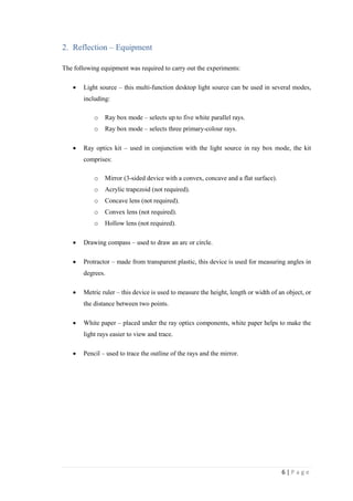
4. Reflection – Results
The following results were obtained during the plane mirror experiment:
Test
Number
Angle of Incidence Angle of Reflection Test Date
Test 1 15 ° 15 ° 20/10/16
Test 2 30 ° 30 ° 20/10/16
Test 3 65 ° 65 ° 20/10/16
Table 1: Plane mirror results.
Question 1: What is the relationship between the angles of incidence and reflection?
Answer 1: The angle of incidence equals the angle of reflection for the same plane of
incidence as indicated by the following formula:
∅𝑖 = ∅ 𝑟 (1)
Question 2: Are the three coloured rays reversed left-to-right by the plane mirror?
Answer 2: The three coloured rays are not reversed by the mirror.
The following results were obtained during the cylindrical mirror experiment:
Concave Mirror Convex Mirror Test Date
Focal length [ f] 63 mm 63 mm 20/10/16
Radius of Curvature [ R] 126 mm 126 mm 20/10/16
Table 2: Cylindrical mirror results.

12 | P a g e
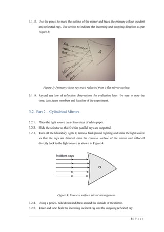
Question 1: What is the relationship between the focal length of a cylindrical mirror and its
radius of curvature? Do your results confirm your answer?
Answer 1: For a cylindrical mirror, the radius of curvature is two times the focal length. The
results in Table 2 confirm this relationship as can be seen when they are fed into the following
formula:
𝑅 = 2𝑓 (2)
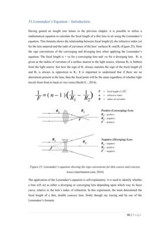
given
radius of curvature 𝑅 = [ 𝑚𝑚 ]
focal length 𝑓 = 63 [ 𝑚𝑚 ]
then
𝑅 = 2×63
𝑅 = 126 𝑚𝑚
Question 2: What is the radius of curvature of the plane mirror?
Answer 2: As there is no focal point where light converges, then the radius of curvature could
be said to approach infinity.

13 | P a g e
5. Reflection – Discussion
The test was repeated three times at different angles of incidence to show that the reflection
law holds true, regardless of the incoming angle. Simply put, the incident ray (incoming), the
reflected ray (outgoing), and the normal to the surface (90 degrees) all lie in the same plane.
Moreover, the reflection angle is equal to the incident angle with respect to the normal to the
mirror. This applies to
As predicted, the plane mirror experiment confirmed that the angle of incidence and reflection
were the same when measured from the normal to surface. In practice, small differences in the
angles were seen during the ray racing and measurement process, but were expected. Small
variances were introduced because of the questionable quality of the light source and the
inaccuracy of the measuring instruments.
The diagram in Figure 2 illustrates the reflection law and further evidence is given using the
formula (1), where the incoming and outgoing angles are shown as equal. Discussion with
other lab groups yielded the same result at different incident angles.
The data gathered during this test conclusively demonstrated how light converges at a focal
point at half the radius of the mirror curvature. Feeding the results into formula (2) produces a
radius, which when set as the distance between the two compass points would draw a perfect
circle that aligns with the mirror curvature. Thus, both the calculation and the results equally
reflect the law. It was noted that for a concave surface the focus point converged at the near
side of the light source. However, for a convex surface, the point of focus had to be established
by elongating the divergent ray traces and was positioned at the far side of the mirror surface.
In both cases, though, the focal point was the same at 63mm, which produced a radius of
126mm.

14 | P a g e
6. Reflection – Conclusion
In conclusion, the team explored the optical phenomena of specular reflection when a light
source was applied to a plane mirror surface. By tracing and evaluating both the incoming and
outgoing rays, the law of reflection was confirmed: the incident angle was equal to the
reflected angle, when measured from the normal to the surface. Moreover, both angles are on
opposite sides of the normal.
Further confirmation of the law of reflection was established during the primary colour ray
experiment. When the ray traces were examined, the same relationship between the incoming
and outgoing rays was seen. Yet again, the reflected angle was proven to be equal to the
incident angle. It was also noted that the primary colour rays did not reverse as they reflected
from the flat mirrored surface, offering even more evidence in support of the law of reflection.
Multiple readings were taken to ensure that the conclusion was not just based upon one
experimental result. It can be concluded then, that the experiment was a success and that
further testing of different incident angles would continue to verify the law of reflection. While
the team’s test results were quite accurate, greater resolution could be achieved by using a
higher quality light source in a much darker room and by using measuring devices which have
smaller increments.
The object of this experiment was to understand how light reacts to a cylindrical mirror with
respect to specular reflection. Interestingly, the ray traces showed that when light reflects from
a concave mirrored surface, it converges on the near side of the mirror at a focal point equal to
half the radius of the curvature. Conversely, applying the same light source to a convex
mirrored surface exhibited a divergent effect. This time, however, the focal point was found to
be on the far side of the mirror surface, established by elongating the divergent reflected ray
path. The law, then, still held true: the radius of the curvature was twice the focal length.
Initially, the cylindrical mirror experiment yielded some inconclusive results as the 5 light
beams were so close together that the ray tracing was difficult to perform. If the distance
between each ray was increased somewhat, the angles would increase allowing easier tracing
and interpretation of the results. Additionally, the low-cost compass was not very repeatable
and multiple scribing’s had to be taken to find the curvature of the cylindrical mirror.

15 | P a g e
While the relationship between light rays and the radius of curvature for a cylindrical mirror
had been established, it was fascinating to consider whether the same relationship was true for
a plane mirror. It is known that to define focal length, light rays travelling along different paths
must come together. This can be interpreted as the notion of parallel light rays meeting at some
distant point. Therefore, the reflection from a flat mirror would never converge and could be
said to approach infinity. Thus, the radius of curvature of a plane mirror would also be infinite
as there is no focus point.

16 | P a g e
7. Snell’s Law – Introduction
Another key property of light is Refraction. Essentially, refraction is the effect brought about
by a reduction in wavelength as light slows down when passing from one material or medium
to another. This point of change is known as the refractive index and is equal to the speed of
light in a vacuum divided by the speed of light in the material. Given that the speed of light is
slower in a material than that of a vacuum, the refractive index is always greater than one.
Figure 8 illustrates how a light beam is bent as it enters a material with a higher index of
refraction (Hecht J. , 2008):
Figure 8: Refraction of light waves as they pass from a low-index medium with refractive
index n1 to a higher-index medium with index n2 ( (Hecht J. , 2008).
Refraction, however, does not occur within the material itself. Visually, the oblique path of
light is bent as it enters a transparent material, and its angle of refraction can be determined by
comparing the direction of incident light with the normal to the surface using Snell’s Law:
𝑛1 sin 𝜃1 = 𝑛2 sin 𝜃2 (3)
In optics, refraction occurs when light passes from one medium boundary to another with
differing refractive indexes at an oblique angle. This theory was used in Experiment 4 to
determine the index of refraction of an acrylic trapezoid by measuring the angles of incidence
and refraction. Refraction applications can be seen in everyday devices such as binocular
lenses, glasses, cameras, fibre-optics and light splitting prisms. More unusual applications even
include forensics.

17 | P a g e
8. Snell’s Law – Equipment
The following equipment was required to carry out the experiment:
 Light source.
 Acrylic trapezoid from ray optics kit.
 Protractor.
 Metric ruler.
 White paper.
 Pencil.

18 | P a g e
9. Snell’s Law – Procedure
The team maintained the same roles as they had in the law of reflection experiments.
9.1. Gather all the necessary equipment for the experiment and set out a clean sheet of
white paper for the experiment to take place upon.
9.2. Plug in the light source and switch it on, then select ray box mode by sliding the ray
selector to single ray.
9.3. Turn off the laboratory lights to remove background lighting and arrange the trapezoid
so the light passes through the parallel sides as shown in Figure 9:
Figure 9: Trapezoid arranged so the incident ray passes through the parallel faces.
9.4. Using a pencil, hold down the trapezoid and draw around the outside. Mark the
position of the incoming incident ray and the outgoing refracted ray.
9.5. Now turn on the laboratory lights and remove the trapezoid and the light source from
the paper.
9.6. On the drawing, indicate ray direction by using arrows and then use the ruler to draw a
line between the points where the ray entered and exited the trapezoid.
9.7. Next, draw the normal to surface with a dotted line at the point where the ray entered
the trapezoid.
9.8. Use the protractor to measure the angle of incidence and refraction from the normal.
Record the results in the first row of Table 3.
9.9. Repeat steps 3 to 9, but reposition the light source to provide a different angle of
incidence. Obtain a total of three sets of results with differing angles of incidence.
9.10. Record any Snell’s Law observations for evaluation later. Note the time, date, team
members and location of the experiment.

19 | P a g e
10.Snell’s Law – Results
Angle of
Incidence
Angle of
Refraction
Calculated Index of
Refraction for Acrylic
Test
Date
26 ° 13 ° 1.95 20/10/16
40 ° 20 ° 1.88 20/10/16
64 ° 32 ° 1.70 20/10/16
Average: 1.84 20/10/16
Table 3: Snell’s Law results showing the calculated index of refraction for acrylic.
Assuming the index of refraction of air is 1.0 (Appendix 1), Snell’s Law (3) can be transposed
to determine the index of refraction of acrylic as follows:
𝑛2 =
𝑛1 sin 𝜃1
sin 𝜃2
given
index of refraction (acrylic) 𝑛2
index of refraction (air) 𝑛1 = 1.0
angle of incidence 𝜃1 = 26 [ ° ]
angle of refraction 𝜃2 = 13 [ ° ]
then
𝑛2 =
1.0 × sin26
sin13
𝑛2 =
0.438371
0.224951
𝑛2 = 1.95
The same formula was applied for each angle of incidence and refraction, and the calculated
index of refraction for acrylic results were fed back into Table 3, above. Then, the results were
averaged out to a value of 𝑛2𝐴𝑉𝐺 = 1.84 by adding them together and dividing by three.
Finally, all three acrylic refractive index results were compared as a percentage difference (𝜎)
to the accepted value of 𝑛2 = 1.5 (Appendix 1) as follows:
𝜎 = (
𝑛2𝐴𝑉𝐺 − 𝑛2
𝑛2
)×100

20 | P a g e
𝜎 = (
1.84 − 1.5
1.5
) ×100
𝜎 = 22.7 % from accepted value
Question 1: What is the angle of the ray that leaves the trapezoid relative to the ray that enters
it?
Answer 1: The ray enters and leaves the trapezoid at the same angle.

21 | P a g e
11.Snell’s Law – Discussion
As expected, when light was shone onto the surface of the acrylic trapezoid, refraction took
place. By looking down upon the trapezoid, it was clear to see the path of light deviation as it
passed through. The ray had left the acrylic trapezoid at the same angle that it had entered.
This occurred because refraction took place from air to acrylic at the entrance, and then again
from acrylic to air at the exit. In effect, the light speed slowed as the index of refraction
increased (𝑛1 < 𝑛2) and then sped up when the index decreased (𝑛1 > 𝑛2).
An interesting observation was made while measuring the incident and refracted angles: the
refracted angle was approximately half that of the incident angle. Given that the accepted
index of refraction is 1.5 for acrylic and 1.0 for air, this made perfect sense as there is a 50%
difference.
It was also noted that the angle had to be oblique or the ray would not exit as predicted. This
phenomenon is an effect brought about because of Critical Angle and Total Internal Reflection
(TIR) and will be discussed in a later experiment. For the purposes of this experiment, an
oblique angle was used.
After the test results were obtained, Snell’s law was used to calculate the index of refraction
for acrylic at differing angles of incidence. However, the calculated index of refraction for
acrylic results gave an average value of 1.84, which was a 22.7 % difference from the accepted
value. This high deviation is likely the result of inaccurate ray tracing or a lack of smaller
protractor increments. Another unlikely contributor could be due to impurities in the acrylic,
such as nitrogen or bromine monomers, which increase refractive index.

22 | P a g e
12.Snell’s Law – Conclusion
It is clear then, that when light passes across the boundary of one transparent material to
another, refraction takes place. This is because there is a change in wavelength speed. The
speed of light in air is faster than that of acrylic, which means the refractive index of air is
lower than acrylic and the light will slow down as it enters the medium. The incident angle of
entry must be oblique for the ray to change direction. Furthermore, the refractive indexes of
the materials have a relationship, where the angle of refraction is related to the angle of
incidence, which is recognised as Snell’s Law. When the incident ray medium has a higher
refractive index than the refracted ray medium, the incident angle is known to be less than the
refracted angle. On the other hand, when the incident ray medium has a lower refractive index
then the refracted ray medium, the incident angle is greater than the refracted angle.
Performed three times, the ray tracings from the trapezoid showed that the entrance and exit
rays were the same. This confirmed the validity of Snell’s Law, as the calculated refractive
index was close to the accepted norm for acrylic. Taking this one step further, the formula was
transposed to determine the refractive index of air, using an acrylic refractive index of 1.84.
The result was 1.0 which is the accepted norm for air.

23 | P a g e
13.Total Internal Reflection – Introduction
Previously we discussed the theory of Snell’s Law with respect to refraction. During the
experiment, it was identified that an incident ray had to approach a transparent material at an
oblique angle for the light to transmit from one medium to another. However, there is scenario
where the refracted ray does not exit the medium. This occurs when a light ray, travelling from
an optically denser medium to an optically rarer medium, is incident at 90 degrees or greater
and is known as the critical angle (Khurana, 2008). Figure 10 shows how refraction occurs
when the critical angle is less than 90 degrees (a). At precisely 90 degrees, the light is refracted
along the refractive boundary between both materials (b). If the critical angle exceeds 90
degrees, the light ray experiences total internal reflection (TIR) and reflects internally (c).
Figure 10: Interaction of light showing the relationship of the incident angle with refraction,
critical angle and total internal reflection (spmphysics.com, 2016).
The study group performed Experiment 5 to verify the total internal reflection theory and
identified the critical angle at which TIR occurred in the acrylic trapezoid. Calculations were
Snell’s law was used to confirm the results. Total internal reflection is used in many
applications around the world and is the premise under which fibre optic telecommunications
are based (Figure 11). Other uses include fibre optic lights, endoscopes, binoculars and many
more.

24 | P a g e
Figure 11: Rays clad in an optical fibre (Hecht E. , 2014)

25 | P a g e
14.Total Internal Reflection – Equipment
 Light source.
 Acrylic trapezoid from ray optics kit.
 Protractor.
 Metric ruler.
 White paper.
 Pencil.

26 | P a g e
15.Total Internal Reflection – Procedure
15.1. Gather all the necessary equipment for the experiment and set out a clean sheet of
white paper for the experiment to take place upon.
15.2. Plug in the light source and switch it on, then select ray box mode by sliding the ray
selector to single ray.
15.3. Turn off the laboratory lights to remove background lighting and arrange the trapezoid
so the incident ray enters at least 2 cm from the tip as shown in Figure 12:
Figure 12: Trapezoid arranged so the incident ray passes through tip.
15.4. Position the trapezoid slowly so that the refracted ray just disappears, where colour
separation occurs. Ideally this will be where the red ray vanishes.
15.5. Using a pencil, hold down the trapezoid and draw around the outside.
15.6. Mark the incoming incident ray and outgoing reflected rays, and the point at which
total internal reflection occurs.
15.7. Now turn on the laboratory lights and remove the trapezoid and the light source from
the paper.
15.8. On the drawing, indicate ray direction by using arrows and then use the ruler to join
the lines between the designated points.
15.9. Extend the lines, so that a protractor can be used to measure the angle between the
incident ray and the reflected ray (Figure 13).
Figure 13: Trapezoid arranged showing the TIR angle.

27 | P a g e
15.10. Record the measured critical angle. It is defined as half the measurement, because the
angle of incidence equals the angle of reflection.
15.11. Calculate the theoretical critical angle using Snell’s Law, using the index of refraction
of acrylic at 1.5.
15.12. Now determine the difference between the measured and theoretical angles as a
percentage.
15.13. Record any observations for evaluation later. Note the time, date, team members and
location of the experiment.

28 | P a g e
16.Total Internal Reflection – Results
During the experiment the measured critical angle was identified as 𝜃𝑐 = 41°.
If the angle of the refracted ray is 90 degrees, the theoretical critical angle can be determined
from Snell’s Law:
𝑛 sin 𝜃𝑐 = 1 sin90°
(4)
transposing for 𝜃𝑐
𝜃𝑐 = 𝑠𝑖𝑛−1
(
1
𝑛
)
given
index of refraction (acrylic) 𝑛 = 1.5
then
𝜃𝑐 = 𝑠𝑖𝑛−1
(
1
1.5
)
𝜃𝑐 = 𝑠𝑖𝑛 −1
0.666
𝜃𝑐 = 41.8°
The percentage difference (𝜎) between the measured and theoretical angles is:
𝜎 = (
𝑡ℎ𝑒𝑜𝑟𝑒𝑡𝑖𝑐𝑎𝑙 𝑐𝑟𝑖𝑡𝑖𝑐𝑎𝑙 𝑎𝑛𝑔𝑙𝑒 − 𝑚𝑒𝑎𝑠𝑢𝑟𝑒𝑑 𝑐𝑟𝑖𝑡𝑖𝑐𝑎𝑙 𝑎𝑛𝑔𝑙𝑒
𝑡ℎ𝑒𝑜𝑟𝑒𝑡𝑖𝑐𝑎𝑙 𝑐𝑟𝑖𝑡𝑖𝑐𝑎𝑙 𝑎𝑛𝑔𝑙𝑒
) ×100
𝜎 = (
41.8 − 41.0
41.8
) ×100
𝜎 = 1.9 %
Question 1: How does the brightness of the internally reflected ray change when the incident
angle changes from less than 𝜃𝑐 to greater than 𝜃𝑐?
Answer 1: The brightness of the ray increases and reaches its maximum intensity when the
angle of incidence increases to become exactly equal to the critical angle. Further increase in
critical angle has no additional effect and the brightness of the ray remains constant as its
whole intensity becomes channelled to internal reflection.

29 | P a g e
Question 2: Is the critical angle greater for red light or violet light? What does this tell you
about the index of refraction?
Answer 2: As wavelength increases, so too, does critical angle. Thus, critical angle is greater
for red light than violet light, because red light has a greater wavelength. Moreover, the index
of refraction decreases when exposed to red light and increases when exposed to violet light.

30 | P a g e
17.Total Internal Reflection – Discussion
The experiment yielded a small difference in the measured critical angle to that of the
theoretical critical angle. A value of 41 degrees was measured for the acrylic material, while
the theoretical value, calculated via Snell’s Law, was 41.8 degrees. Though acceptable, the
difference of 1.9% was likely the result of the difficulty involved in setting the trapezoid to the
point where the red ray disappeared. This was very much prone to misalignment as there was a
tolerance where the change in colour took place. Another key issue was the protractor could
only measure in 1 degree increments. A repeat of the test could be made with a more accurate
protractor to improve the results.
It was obvious from the experiment, that TIR occurred when the incident angle became greater
than the critical angle of 90 degrees. The incident light ray was viewed from above as it
entered, reflected internally, and then exited the trapezoid without refraction taking place.
Likewise, when the incident angle was equal to the critical angle of 90 degrees, refraction took
place along the refractive boundary of the materials and TIR did not occur.
Another point to note, when positioning the trapezoid so that TIR took place, was that the red
ray was the last visible light to disappear. Therefore, it can be said that its refractive index was
smaller than that of violet light.

31 | P a g e
18.Total Internal Reflection – Conclusion
By varying the angle of the incoming incident ray to the trapezoid, it was possible to see a
change in refraction, brought about by equalling the critical angle of 90 degrees. Increasing the
angle beyond 90 degrees demonstrated how TIR prevented refraction. Snell’s Law was used to
prove the critical angle for acrylic was 41.8 degrees. Moreover, incident light at the medium
boundary with an angle less than 41.8 degrees was partially transmitted, while angles larger
than 41.8 degrees were internally reflected. This relationship is only true when light in a
medium with a greater index reaches a boundary of a medium with a lower index of refraction.
This association is noteworthy because TIR can be used in everyday applications such as fibre-
optic communications and endoscopy.
Another point of interest, was the intensity of the internally reflected incident light. The closer
the ray approached critical angle, the more intense the light became. When critical angle was
reached, maximum intensity was also reached. Once TIR took place, the light intensity
remained at its maximum.

32 | P a g e
19.Dispersion – Introduction
In the previous report, Snell’s Law was used to show the relationship between the indexes of
refraction of two transparent mediums and the angles of incidence and refraction. This effect is
known as refraction. However, a variance in wavelength or light speed will have a different
index of refraction within the same material, causing visible light (Figure 14) to refract at
different angles (Born & Wolf, 1999). This phenomenon is called dispersion and is evidenced
in everyday life as the rainbow.
Figure 14: Visible light spectrum (Reusch, 2016).
In 1966, Newton first discovered how white light could be split into the colours of the
spectrum by means of a prism (Born & Wolf, 1999). Figure 15, depicts how a white ray of
light, made up of seven colours, refracts when it strikes the surface of the prism and slows
down. Inside the prism, each individual colour refracts at a different angle and disperses into
the visible light spectrum. As the rays exit the prism, they speed up once more as light travels
faster in air than glass. Note how the red light refracts less than that of violet because its
wavelength is higher with respect to the normal to the surface.
Figure 15: The dispersion effect through a prism (Dispersion of light, 2016).
The following dispersion experiment supports the theory behind dispersion, defining the index
of refraction of acrylic for blue and red light in the same material.

33 | P a g e
20.Dispersion – Equipment
 Light source.
 Acrylic D-shaped Lens.
 Ray table.
 White paper.
 Pencil.

34 | P a g e
21.Dispersion – Procedure
21.1. Plug in the light source and switch it on, then place it on a sheet of white paper.
21.2. Select ray box mode by sliding the ray selector to single ray.
21.3. Turn off the laboratory lights to remove background lighting and align the light source
so that the beam of white light crosses the normal or the ray table as shown in Figure
16:
Figure 16: D-shaped lens arrangement on a ray table.
21.4. Now place the acrylic D-shaped lens in the semi-circle on the ray table.
21.5. Ensure the angle of incidence is set to 0 degrees by turning the ray table so that the
light passes through the curved surface of the acrylic lens.
21.6. Next, have your lab partner to hold the white paper to provide a backdrop for the
outgoing ray by holding it vertically close to the ray table’s edge.
21.7. Increase the angle of incidence by rotating the table slowly, making sure to hold the
bottom firmly while turning the top. Observe how refraction takes place at the flat
surface, but not at the curved surface. Also, pay close attention to the refracted light on
the paper as the angle of incidence is increased as shown in Figure 17:
Figure 17: Demonstration of dispersion through a D-shaped lens.
21.8. Turn on the laboratory lights and record any dispersion observations for evaluation
later. Be sure to note the time, date, team members and location of the experiment.

35 | P a g e
22.Dispersion – Results
Question 1: At what angle of refraction do you notice colour separation in the refracted light?
Answer 1: At approximately 42°, the team observed colour separation. This seemed to vary
slightly between different lab groups, because of the variance in background light in different
areas of the room.
Question 2: At what angle of refraction does the maximum colour separation occur?
Answer 2: Maximum colour separation occurred between 80 to 85°. Interestingly, it was
noticed that when the angle of refraction was further increased, total internal reflection took
place.
Question 3: What colours are present in the refracted ray? (Write them in the order of
minimum to maximum angle of refraction.)
Answer 3: As the angle of refraction varied from minimum to maximum, the following colours
were observed in the refracted ray: red, cyan, blue and violet. The other visible light spectrum
colours were not observed due to the quality of the room lighting.
Question 4: Use Snell’s Law (Equation 11.1) to calculate the index of refraction of acrylic for
red light (n red) and the index of refraction for blue light (n blue).
Answer 4: The refracted red light was observed at 80° and the refracted blue light was noticed
at 84°. At an incident angle of 42°, Snell’s law (3) could be used in both cases to calculate
each index of refraction for acrylic to air (n2 = 1.0) as the ray exits the lens:
transposing (3) for 𝑛1
𝑛1 =
𝑛2 sin 𝜃2
sin 𝜃1
given
index of refraction (acrylic) 𝑛1(𝑟𝑒𝑑) =

36 | P a g e
then
𝑛1(𝑟𝑒𝑑) =
1.0 × sin 80
sin 42
𝑛1(𝑟𝑒𝑑) =
0.9848
0.6691
𝑛1(𝑟𝑒𝑑) = 1.472
Similarly, using equation (1), the index of refraction for blue light was calculated to be:
given
index of refraction (acrylic) 𝑛1(𝑏𝑙𝑢𝑒) =
then
𝑛1(𝑏𝑙𝑢𝑒) =
1.0 × sin84
sin 42
𝑛1(𝑏𝑙𝑢𝑒) =
0.9945
0.6691
𝑛1(𝑏𝑙𝑢𝑒) = 1.486

37 | P a g e
23.Dispersion – Discussion
During the test, it was noted that the ray only refracted at the flat surface of the lens. Colour
separation was first noticed at 42°, whereby maximum colour separation occurred at 85°.
Further increase in angle resulted in total internal reflection. Visibly, it was seen that the red
light had a smaller angle of refraction than the blue light which supported the dispersion theory
that blue light refracts more due to its lower wavelength.
Snell’s law was used to calculate the index of refraction of acrylic at an incident angle of 42°,
for both red and blue light. At n = 1.472, red light had a lower index of refraction than that of
blue light at 1.486. This was to be expected as red light has a lower frequency and higher
wavelength. From these results, one can confirm that the higher the index of refraction, the
slower the speed of light travelled through the medium. Blue light moved slower through the
acrylic than red light.
The experiment had to be attempted several times as it was very difficult to observe the
dispersion effect because the difference the angles of refraction for each colour was very small
through the D-shaped lens. This experiment could be made easier by using a glass prism
instead.

38 | P a g e
24.Dispersion – Conclusion
It can be concluded that visible light is made up of a collection of component colours, which
disperse inside the acrylic lens. The angles of dispersion vary with wavelength with respect to
the index of refraction in acrylic, which is slightly different for each colour. Snell’s law
showed how the refractive index of acrylic was different for different wavelengths of light. It
was confirmed that the higher wavelength light resulted in a lower refractive index and smaller
angle of refraction. Thus, red light had a smaller refractive index than blue light.
In fibre-optic communications, dispersion is an undesirable effect. This is because different
colours of light travel at different speeds through the same medium. In the digital world, this
would mean that it is harder to distinguish between a logic 1 and logic 0, resulting in bit errors.

39 | P a g e
25.Convex and Concave Lenses – Introduction
Lenses have been around a very long time. In ages past, the classic manmade lens was used to
start a fire, which is today recognised as the magnifying glass. At its core, a lens is a refracting
device, which can either disperse or focus light. There are countless applications for lenses and
they are usually categorised as having two or more refracting interfaces, with at least one being
curved. There are two main types (Hecht E. , 2014):
 Simple lens – is made up of one element to include two refracting surfaces.
 Compound lens – comprises of more than one element.
Additionally, Hecht (2104) explains there are convex or converging lenses of various types,
which are thicker in the middle than at the edges. Or, there are concave or diverging lenses,
which are thinner in the centre, Figure 18:
Figure 18: Cross section of various centred simple spherical lenses (Hecht E. , 2014).
Concave lenses are used to aide short-sightedness or myopia as they divert light, causing
objects to appear father way. The reverse is said of convex lenses, whereby near-sightedness is
improved as items appear larger because the light rays are focused. Classic examples are the
concave side mirror on a car, which makes one think objects are closer than they are, and the
convex camera lens, which focus light rays at the subject which is being captured. While
technology is a great example of what lenses can be used for, the greatest of all lenses is of
course the human eye.
This experiment is founded on these principles, examining the difference between a convex
and concave lens and confirming the focal length of each. The results show how when used
together, the lenses can correct the refracted rays from one lens to another and maintain
parallel incoming and outgoing ray path while varying the spacing between rays.

40 | P a g e
26.Convex and Concave Lenses – Equipment
 Light source.
 Convex lens.
 Concave lens.
 Metric ruler.
 White paper.
 Pencil.

41 | P a g e
27.Convex and Concave Lenses – Procedure
27.2. Select ray box mode by sliding the ray selector to output three parallel rays.
so that the beams of white light shines into the convex lens, which is standing on its
flat edge, as shown in Figure 19:
Figure 19: Convex lens arrangement.
27.4. Using a pencil, hold down the convex lens and draw around the outside. Mark the
position of the incoming incident rays and the outgoing refracted rays.
27.5. Now turn on the laboratory lights and remove the convex lens and light source from
the paper.
27.6. Mark the focal point, where the three rays converge and cross one another, as
indicated in Figure 20.
Figure 20: Convex lens focus point.
27.7. Using the ruler, measure the distance from the focal point to the centre of the convex
lens and record the results in Table 4.
27.8. Repeat steps 1 to 7 for the concave lens, noting that in step 6 the reflected rays will
diverge instead of converge. A ruler will be required to elongate the lines so that they
converge at a focus point behind the lens (Figure 21). Be sure to record the focal
length as a negative number.

42 | P a g e
Figure 21: Concave lens focus point.
27.9. Now, arrange both the concave and convex lenses in the path of the three rays as can
be seen in Figure 22:
Figure 22: Nested concave and convex lens arrangement.
27.10. Using a pencil, hold down the lenses and draw around the outside. Mark the position
of the incoming incident rays and the outgoing refracted rays. You should obtain a
result like the illustration in Figure 23:
Figure 23: Incident and refracted rays for nested concave and convex lenses.
27.11. Record your observations and then slide the concave lens away from the convex lens,
noting the effect on the rays.
27.12. Now, reverse the order of the lenses and compare the effects.
27.13. Turn on the laboratory lights and record any observations for evaluation later. Be sure
to note the time, date, team members and location of the experiment.

43 | P a g e
28.Convex and Concave Lenses – Results
The following results were obtained during the convex and concave lenses experiment:
Concave Lens Convex Lens Test Date
Focal length [ f] 120mm -118 mm 17/11/16
Table 4: Convex and concave lenses results.
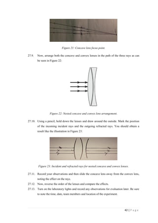
Question 1: When the convex and concave lenses are nested together, are the outgoing rays
converging, diverging or parallel? What does this tell you about the relationship between the
focal lengths of these two lenses?
Answer 1: It is clear from the image in Figure 23, that the incoming and outgoing rays are
almost parallel. This indicated that the lenses have focal lengths that have almost equal
magnitude, yet opposing sign.
Question 2: When the convex and concave lenses are nested together, what is the effect of
changing the distance between the lenses? What is the effect of reversing their positions?
Answer 2: Figure 24 shows that by moving the lenses apart the distance between each output
ray will vary, but the rays remain almost parallel. Reversing the lens order has the same net
effect, though obviously, the rays would diverge instead of converge between both lenses
when the light source strikes the concave lens first:
Figure 24: Ray tracing of a convex and concave lens arrangement, showing narrower spacing
between the rays at the output of the concave lens that at the input of the convex lens.

44 | P a g e
29.Convex and Concave Lenses – Discussion
The experiment verified the fundamental principle of lenses: when light passed through a lens,
it either converged at a focal point if the lens was convex, or diverged if the lens was concave.
Both lenses had the same radius of curvature, which became evident when the lenses were
nested together. Measuring the focal length of each lens yielded approximately the same focal
length, but in opposing directions, so the concave lens result was indicated with a negative
sign. Also, the input and output rays were observed to be near enough parallel, since one lens
corrects the other as their radius of curvature is the same.
When the lenses were spaced apart, the incoming and outgoing rays remained parallel, but the
distance between the rays varied. If light struck the convex lens before the concave lens, then
the spacing between the output rays was narrower because the rays converged to the entry
point of the concave lens. The opposite scenario took place when light struck the concave lens
first, because the light diverged into the convex lens instead. Thus, the output rays in this case
were wider spaced. One other point of interest was noted. If you moved the concave lens away
from the light source and placed it beyond the focus point, the output rays diverged instead of
remaining parallel as the convex lens no longer corrected the rays.
It was quite difficult to observe the variance in spacing between the parallel output rays during
the experiment. It could be improved by using a light source with wider spacing and larger
lenses.

45 | P a g e
30.Convex and Concave Lenses – Conclusion
One can conclude that the lenses had two fundamental refractive properties: convex lenses
converge light at a point of focus and concave lenses diverge light. Also, the focus point of a
converging lens is expressed as a positive number and is on the outgoing side of the lens.
Whereas, the focus point of a diverging lens is given a negative sign and is on the same side as
the incoming rays, which have been projected back to the centre. Furthermore, by nesting both
lenses together, it was possible to make the incoming parallel light equal the outgoing parallel
light because the focal lengths were equal, but opposing. Finally, it was possible to vary the
distance between the rays by spacing apart the lenses.

46 | P a g e
31.Lensmaker’s Equation – Introduction
Having gained an insight into lenses in the previous chapter, it is possible to utilise a
mathematical equation to calculate the focal length of a thin lens in air using the Lensmaker’s
equation. This formula shows the relationship between focal length (f), the refractive index (n)
for the lens material and the radii of curvature of the lens’ surfaces R1 and R2 (Figure 25). Note
the sign conventions of the converging and diverging lens when applying the Lensmaker’s
equation. The focal length is + ve for a converging lens and -ve for a diverging lens. R1 is
given as the radius of curvature of a surface nearest to the light source, whereas R2 is farthest
from the light source. See how the sign of R1 always matches the sign of the focal length (f)
and R2 is always in opposition to R1. It is important to understand that if there are no
aberrations present in the lens, then the focal point will be the same regardless of whether light
travels from front to back or vice versa (Hecht E. , 2014).
Figure 25: Lensmaker’s equation showing the sign conventions for thin convex and concave
lenses (meritnation.com, 2016)
The application of the Lensmaker’s equation is self-explanatory: it is used to identify whether
a lens will act as either a diverging or converging lens depending upon which way its faces
curve, relative to the lens’s index of refraction. In this experiment, the team determined the
focal length of a thin, double concave lens, firstly though ray tracing and by use of the
Lensmaker’s formula.

47 | P a g e
32.Lensmaker’s Equation – Equipment
 Light source.
 Thin double concave lens.
 Metric ruler.
 White paper.
 Pencil.

48 | P a g e
33.Lensmaker’s Equation – Procedure
33.2. Select ray box mode by sliding the ray selector to output three parallel rays.
so that the beams of white light shines into the double concave lens, which is standing
on its flat edge, as shown in Figure 26:
Figure 26: Double concave lens arrangement.
33.4. Using a pencil, hold down the double concave lens and draw around the outside. Mark
the position of the incoming incident rays and the outgoing refracted rays.
33.5. Now turn on the laboratory lights and remove the double concave lens and light source
from the paper.
33.6. Mark the focal point, by extending the outgoing divergent rays back through the lens
to where they cross.
33.7. Using the ruler, measure the distance from the focal point to the centre of the double
concave lens and record the results in Table 5 as a negative value.
33.8. Turn off the lights once more and place the lens in front of the light box once again.
Notice, the faint reflected rays off the first surface. Mark the focal point, where the
faint reflected rays converge and cross one another.
33.9. Using the ruler, measure the distance from the reflected ray focal point to the centre of
the concave mirror and record the radius of curvature in Table 5. Radius of curvature
is twice the distance as indicated in Figure 27:
Figure 27: Reflected ray trace from the surface of the double concave lens.
33.10. Turn on the laboratory lights and record any observations for evaluation later. Be sure
to note the time, date, team members and location of the experiment.

49 | P a g e
34.Lensmaker’s Equation – Results
The following results were obtained during the Lensmaker’s equation experiment:
Concave Mirror Test Date
Measured focal length [ f] -120 mm 20/10/16
Radius of Curvature [ R1]
(Measured reflected rays are
treated like a concave mirror.
Calculated as twice focal length)
-121 mm 20/10/16
Table 5: Lensmaker’s equation results.
Question 1: Calculate the focal length of the lens using the Lensmaker’s equation. The index
of refraction is 1.5 for the acrylic lens. Remember that a concave surface has a negative radius
of curvature?
Answer 1: Assuming the curvature of both sides is equal and R1 is -ve and R2 is +ve, where R1
and R2 are equal radii, the Lensmaker’s equation can be used to determine the focal point of a
thin concave lens as follows:
1
𝑓
= (𝑛 − 1) (
1
𝑅1
−
1
𝑅2
) (5)
transposing for the focal point ( f )
𝑓 =
1
(𝑛 − 1) (
1
𝑅1
−
1
𝑅2
)
given
index of refraction (acrylic) 𝑛 = 1.5
radius of curvature 𝑅1 = −121 [ 𝑚𝑚 ]
radius of curvature 𝑅2 = 121 [ 𝑚𝑚 ]
then
𝑓 =
1
(1.5 − 1) (
1
−121 −
1
121)

50 | P a g e
𝑓 =
1
0.5×(−0.00826 − 0.00826)
𝑓 =
1
0.5×−0.01652
𝑓 =
1
−0.00826
𝑓 = −121.1 𝑚𝑚
Question 2: Calculate the percentage difference between the measured and calculated value of
(f).
Answer 2: The percentage difference (𝜎) between the measured and theoretical focus points is:
𝜎 = (
𝑡ℎ𝑒𝑜𝑟𝑒𝑡𝑖𝑐𝑎𝑙 𝑓𝑜𝑐𝑎𝑙 𝑙𝑒𝑛𝑔𝑡ℎ − 𝑚𝑒𝑎𝑠𝑢𝑟𝑒𝑑 𝑓𝑜𝑐𝑎𝑙 𝑙𝑒𝑛𝑔𝑡ℎ
𝑡ℎ𝑒𝑜𝑟𝑒𝑡𝑖𝑐𝑎𝑙 𝑓𝑜𝑐𝑎𝑙 𝑙𝑒𝑛𝑔𝑡ℎ
) ×100
𝜎 = (
−121.1 − (−120)
−121.1
) ×100
𝜎 = 0.9 %

51 | P a g e
35.Lensmaker’s Equation – Discussion
During the ray tracing stage of the experiment, the measured focal length was determined to be
-120 mm. While the distance was not verified until later, the expected direction was satisfied
as the theory for a concave, diverging lens was supposed to be negative. Next, the radius of
curvature was determined by treating the front of the lens like a concave mirror and tracing
back the faint reflections to the centre where they crossed. This point was then measured to the
surface of the lens and doubled to calculate the lens curvature. At -121 mm, this too met our
expectations. Given that the double concave lens was symmetrical with no aberrations, the
radius of curvature was the same for both sides. These dimensions were used in the
Lensmaker’s equation to calculate and verify a focal point of -121.1 mm, taking great care to
get the concave sign conventions right. The difference between the measured and calculated
results was only 0.9 %, which is quite accurate. This proved that the manual ray tracing
method and the Lensmaker’s equation calculation were performed correctly.

52 | P a g e
36.Lensmaker’s Equation – Conclusion
The Lensmaker’s equation can be used for the design and verification of lenses, and was used
to confirm the measured experiment results of a thin, acrylic double concave lens. The results
show, conclusively, that the focal length of the diverging lens was -120 mm. In the calculation,
the sign convention rules were used on the radii of curvature, so that R1 was closest to the light
source and negative, relative to centre of the lens. Whereas, R2 was furthest from the light
source and positive, relative to the centre of the lens. Additionally, the focal point was
negative, again, confirming the sign convention for a diverging lens. It was clear from the
percentage difference calculation that the experiment had been conducted properly as there
was very little difference in the measured and theoretical values. Finally, the law of reflection
for a concave mirror was also proven, as this was used to obtain the radius of curvature.

53 | P a g e
37.References
Born, M., & Wolf, E. (1999). Principles of Optics. Cambridge: Cambridge University Press.
Dispersion of light. (2016, Novemeber 19). Retrieved from http://physics.tutorvista.com/:
http://physics.tutorvista.com/light/dispersion-of-light.html
Greivenkamp, J. E. (2004). Geometrical Optics. Washington: SPIE Press.
Hecht, E. (2014). Optics. Essex: Pearson Education Limited.
Hecht, J. (2008). Understanding Lasers: An Entry-Level Guide. New Jersey: IEEE Press.
Khurana, A. (2008). Theory and Practice of Optics and Refraction. New Delhi: Elsevier.
meritnation.com. (2016, November 19). Lensmaker's formula. Retrieved from
meritnation.com: http://www.meritnation.com/
Reusch, W. (2016, September 15). Visible and Ultraviolet Spectroscopy. Retrieved from
Chemistry MSU:
https://www2.chemistry.msu.edu/faculty/reusch/virttxtjml/spectrpy/uv-
vis/spectrum.htm
spmphysics.com. (2016, Novemeber 13). Total Internal Reflection and Critical Angle.
Retrieved from spmphysics.onlinetuition.com.my:
http://spmphysics.onlinetuition.com.my/2013/07/total-internal-reflection-and-
critical.html

54 | P a g e
38.Appendix 1 – Index of Refraction for Various Media

55 | P a g e
39.Appendix 2 – Experiment Photographs

NG3D902 - Basic Ray Optics Experiments - 2016

More Related Content

What's hot

Similar to NG3D902 - Basic Ray Optics Experiments - 2016

NG3D902 - Basic Ray Optics Experiments - 2016