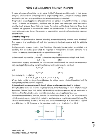
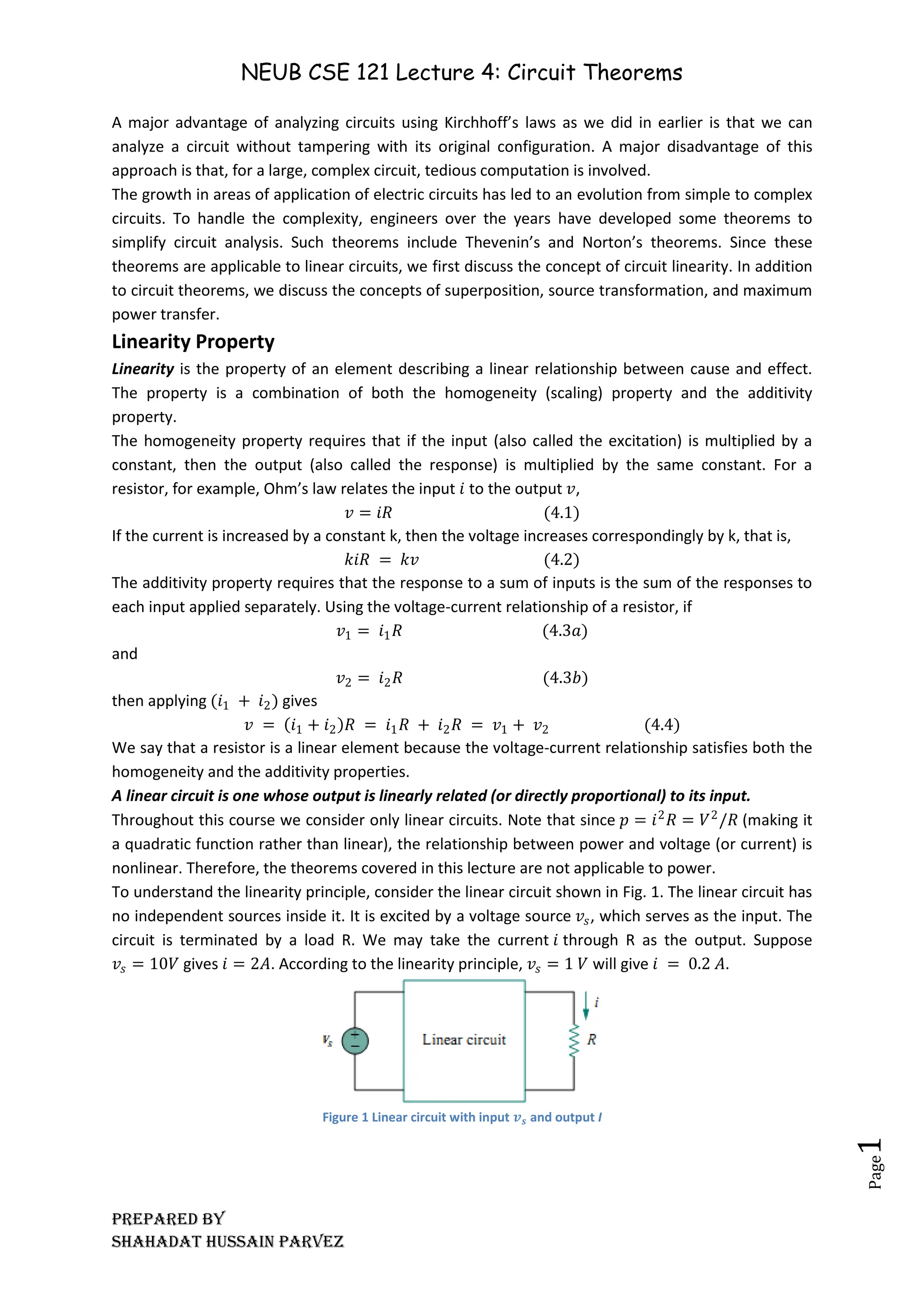
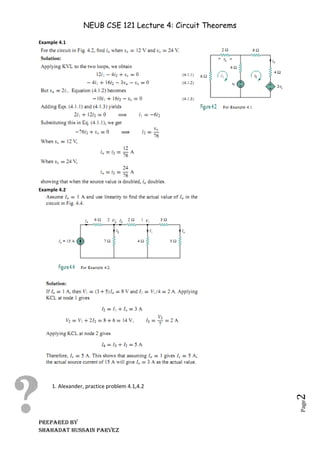
NEUB CSE 121 Lecture 4: Circuit Theorems
Prepared BY
Shahadat Hussain Parvez
Page
1
A major advantage of analyzing circuits using Kirchhoff’s laws as we did in earlier is that we can
analyze a circuit without tampering with its original configuration. A major disadvantage of this
approach is that, for a large, complex circuit, tedious computation is involved.
The growth in areas of application of electric circuits has led to an evolution from simple to complex
circuits. To handle the complexity, engineers over the years have developed some theorems to
simplify circuit analysis. Such theorems include Thevenin’s and Norton’s theorems. Since these
theorems are applicable to linear circuits, we first discuss the concept of circuit linearity. In addition
to circuit theorems, we discuss the concepts of superposition, source transformation, and maximum
power transfer.
Linearity Property
Linearity is the property of an element describing a linear relationship between cause and effect.
The property is a combination of both the homogeneity (scaling) property and the additivity
property.
The homogeneity property requires that if the input (also called the excitation) is multiplied by a
constant, then the output (also called the response) is multiplied by the same constant. For a
resistor, for example, Ohm’s law relates the input 𝑖 to the output 𝑣,
𝑣 = 𝑖𝑅 (4.1)
If the current is increased by a constant k, then the voltage increases correspondingly by k, that is,
𝑘𝑖𝑅 = 𝑘𝑣 (4.2)
The additivity property requires that the response to a sum of inputs is the sum of the responses to
each input applied separately. Using the voltage-current relationship of a resistor, if
𝑣1 = 𝑖1𝑅 (4.3𝑎)
and
𝑣2 = 𝑖2𝑅 (4.3𝑏)
then applying (𝑖1 + 𝑖2) gives
𝑣 = 𝑖1 + 𝑖2 𝑅 = 𝑖1𝑅 + 𝑖2𝑅 = 𝑣1 + 𝑣2 (4.4)
We say that a resistor is a linear element because the voltage-current relationship satisfies both the
homogeneity and the additivity properties.
A linear circuit is one whose output is linearly related (or directly proportional) to its input.
Throughout this course we consider only linear circuits. Note that since 𝑝 = 𝑖2
𝑅 = 𝑉2
/𝑅 (making it
a quadratic function rather than linear), the relationship between power and voltage (or current) is
nonlinear. Therefore, the theorems covered in this lecture are not applicable to power.
To understand the linearity principle, consider the linear circuit shown in Fig. 1. The linear circuit has
no independent sources inside it. It is excited by a voltage source 𝑣𝑠, which serves as the input. The
circuit is terminated by a load R. We may take the current 𝑖 through R as the output. Suppose
𝑣𝑠 = 10𝑉 gives 𝑖 = 2𝐴. According to the linearity principle, 𝑣𝑠 = 1 𝑉 will give 𝑖 = 0.2 𝐴.
Figure 1 Linear circuit with input 𝒗𝒔 and output I
NEUB CSE 121 Lecture 4: Circuit Theorems
Prepared BY
Shahadat Hussain Parvez
Page
2
Example 4.1
Example 4.2
1. Alexander, practice problem 4.1,4.2
NEUB CSE 121 Lecture 4: Circuit Theorems
Prepared BY
Shahadat Hussain Parvez
Page
3
Superposition Theorem
If a circuit has two or more independent sources, one way to determine the value of a specific
variable is to determine the contribution of each independent source to the variable and then add
them up. The approach is known as the superposition.
The superposition principle states that the voltage across (or current through) an element in a
linear circuit is the algebraic sum of the voltages across (or currents through) that element due to
each independent source acting alone.
The principle of superposition helps us to analyze a linear circuit with more than one independent
source by calculating the contribution of each independent source separately. However, to apply the
superposition principle, we must keep two things in mind:
1. We consider one independent source at a time while all other independent sources are
turned off. This implies that we replace every voltage source by 0 V (or a short circuit), and
every current source by 0 A (or an open circuit). This approach is shown in figure 2
2. Dependent sources are left intact because they are controlled by circuit variables.
Figure 2 Removing effect of practical sources
The superposition theorem can be summarized in the following three steps
1. Turn off all independent sources except one source. Find the output (voltage or current)
due to that active source using nodal or mesh analysis.
2. Repeat step 1 for each of the other independent sources.
3. Find the total contribution by adding algebraically all the contributions due to the
independent sources.
Analyzing a circuit using superposition has one major disadvantage: it may very likely involve more
work. If the circuit has three independent sources, we may have to analyze three simpler circuits
each providing the contribution due to the respective individual source. However, superposition
does help reduce a complex circuit to simpler circuits through replacement of voltage sources by
short circuits and of current sources by open circuits.
Since superposition is based on linearity, it is not applicable to the effect on power due to each
source, because the power absorbed by a resistor depends on the square of the voltage or current. If
the power value is needed, the current through (or voltage across) the element must be calculated
first using superposition.
Example 4.3
NEUB CSE 121 Lecture 4: Circuit Theorems
Prepared BY
Shahadat Hussain Parvez
Page
4
Example 4.4
NEUB CSE 121 Lecture 4: Circuit Theorems
Prepared BY
Shahadat Hussain Parvez
Page
5
2. Alexander Example 4.5
3. Alexander Practice Problem 4.3,4.4,4.5
NEUB CSE 121 Lecture 4: Circuit Theorems
Prepared BY
Shahadat Hussain Parvez
Page
6
Source Transformation
We have noticed that series-parallel combination and wye-delta transformation help simplify
circuits. Source transformation is another tool for simplifying circuits. Basic to these tools is the
concept of equivalence. An equivalent circuit is one whose v-i characteristics are identical with the
original circuit.
Previously, we saw that node-voltage (or mesh-current) equations can be obtained by mere
inspection of a circuit when the sources are all independent current (or all independent voltage)
sources. It is therefore expedient in circuit analysis to be able to substitute a voltage source in series
with a resistor for a current source in parallel with a resistor, or vice versa, as shown in Fig. 3. Either
substitution is known as a source transformation.
Figure 3 Transformation of independent Sources
A source transformation is the process of replacing a voltage source 𝒗𝒔 in series with a resistor R
by a current source 𝒊𝒔 in parallel with a resistor R, or vice versa.
The voltage current relationship can be found using the formula
𝑣𝑠 = 𝑖𝑠𝑅 𝑜𝑟 𝑖𝑠 =
𝑣𝑠
𝑅
(4.5)
Source transformation also applies to dependent sources, provided we carefully handle the
dependent variable. As shown in Fig. 4, a dependent voltage source in series with a resistor can be
transformed to a dependent current source in parallel with the resistor or vice versa.
Figure 4 Transformation of Dependent sources
Like the wye-delta transformation studied earlier, a source transformation does not affect the
remaining part of the circuit. When applicable, source transformation is a powerful tool that allows
circuit manipulations to ease circuit analysis. However, we should keep the following points in mind
when dealing with source transformation.
1. Note from Fig. 3 (or Fig. 4) that the arrow of the current source is directed toward the
positive terminal of the voltage source.
2. Note from Eq. (4.5) that source transformation is not possible when 𝑅 = 0, which is the
case with an ideal voltage source. However, for a practical, non-ideal voltage source, 𝑅 ≠ 0.
Similarly, an ideal current source with 𝑅 = ∞ cannot be replaced by a finite voltage source.
Example 4.6
NEUB CSE 121 Lecture 4: Circuit Theorems
Prepared BY
Shahadat Hussain Parvez
Page
7
Example 4.7
NEUB CSE 121 Lecture 4: Circuit Theorems
Prepared BY
Shahadat Hussain Parvez
Page
8
4. Alexander Practice Problem 4.6,4.7
NEUB CSE 121 Lecture 4: Circuit Theorems
Prepared BY
Shahadat Hussain Parvez
Page
9
Thevenin’s Theorem
It often occurs in practice that a particular element in a circuit is variable (usually called the load)
while other elements are fixed. As a typical example, a household outlet terminal may be connected
to different appliances constituting a variable load. Each time the variable element is changed, the
entire circuit has to be analyzed all over again. To avoid this problem, Thevenin’s theorem provides a
technique by which the fixed part of the circuit is replaced by an equivalent circuit.
According to Thevenin’s theorem, the linear circuit in Fig. 5(a) can be replaced by that in Fig. 5(b).
(The load in Fig. 5 may be a single resistor or another circuit.) The circuit to the left of the terminals
a-b in Fig. 5(b) is known as the Thevenin equivalent circuit;
Figure 5 Replacing a linear two-terminal circuit by its Thevenin equivalent: (a) original circuit, (b) the Thevenin
equivalent circuit.
Thevenin’s theorem states that a linear two-terminal circuit can be replaced by an equivalent circuit
consisting of a voltage source 𝑉𝑇ℎ in series with a resistor 𝑅𝑇ℎ, where 𝑉𝑇ℎ is the open-circuit voltage
at the terminals and 𝑅𝑇ℎ is the input or equivalent resistance at the terminals when the independent
sources are turned off.
For the purpose of analyzing the circuit we have to find Thevenin equivalent voltage 𝑉𝑇ℎ and
resistance 𝑅𝑇ℎ.
To do so, suppose the two circuits in Fig. 5 are equivalent. Two circuits are said to be equivalent if
they have the same voltage-current relation at their terminals. Let us find out what will make the
two circuits in Fig. 5 equivalent. If the terminals a-b are made open-circuited (by removing the load),
no current flows, so that the open-circuit voltage across the terminals a-b in Fig. 5(a) must be equal
to the voltage source 𝑉𝑇ℎ in Fig. 5(b), since the two circuits are equivalent. Thus 𝑉𝑇ℎ is the open-
circuit voltage across the terminals as shown in Fig. 6(a); that is,
𝑉𝑇ℎ = 𝑣𝑜𝑐 4.6
Figure 6 Finding 𝑽𝑻𝒉 and 𝑹𝑻𝒉
Again, with the load disconnected and terminals a-b open-circuited, we turn off all independent
sources. The input resistance (or equivalent resistance) of the dead circuit at the terminals a-b in Fig.
5(a) must be equal to 𝑅𝑇ℎ in Fig. 5(b) because the two circuits are equivalent. Thus, 𝑅𝑇ℎ is the input
resistance at the terminals when the independent sources are turned off, as shown in Fig. 6(b); i.e.
𝑅𝑇ℎ = 𝑅𝑖𝑛 (4.7)
NEUB CSE 121 Lecture 4: Circuit Theorems
Prepared BY
Shahadat Hussain Parvez
Page
10
To apply this idea in finding the Thevenin resistance 𝑅𝑇ℎ, we need to consider two cases.
CASE 1: If the network has no dependent sources, we turn off all independent sources. 𝑅𝑇ℎ is the
input resistance of the network looking between terminals a and b, as shown in Fig. 6(b).
CASE 2: If the network has dependent sources, we turn off all independent sources. As with
superposition, dependent sources are not to be turned off because they are controlled by circuit
variables. We apply a voltage source 𝑣𝑜at terminals a and b and determine the resulting current 𝑖𝑜.
Then 𝑅𝑇ℎ = 𝑣𝑜/𝑖𝑜 , as shown in Fig. 7(a). Alternatively, we may insert a current source 𝑖𝑜 at
terminals a-b as shown in Fig. 7(b) and find the terminal voltage 𝑣𝑜. Again 𝑅𝑇ℎ = 𝑣𝑜/𝑖𝑜. Either of the
two approaches will give the same result. In either approach we may assume any value of 𝑣𝑜 and 𝑖𝑜.
For example, we may use 𝑣𝑜 = 1𝑉 𝑜𝑟 𝑖𝑜 = 1𝐴, or even use unspecified values of 𝑣𝑜 𝑜𝑟 𝑖𝑜.
Figure 7 Finding 𝑹𝑻𝒉 when circuit has dependent sources
It often occurs that 𝑅𝑇ℎ takes a negative value. In this case, the negative resistance (𝑣 = −𝑖𝑅)
implies that the circuit is supplying power.
Thevenin’s theorem is very important in circuit analysis. It helps simplify a circuit. A large circuit may
be replaced by a single independent voltage source and a single resistor. This replacement technique
is a powerful tool in circuit design.
As mentioned earlier, a linear circuit with a variable load can be replaced by the Thevenin
equivalent, exclusive of the load. The equivalent network behaves the same way externally as the
original circuit. Consider a linear circuit terminated by a load RL, as shown in Fig. 8(a). The current IL
through the load and the voltage VL across the load are easily determined once the Thevenin
equivalent of the circuit at the load’s terminals is obtained, as shown in Fig. 8(b). From Fig. 8(b), we
obtain
𝐼𝐿 =
𝑉𝑇ℎ
𝑅𝑇ℎ + 𝑅𝐿
4.8𝑎
𝑉𝐿 = 𝑅𝐿𝐼𝐿 =
𝑅𝐿
𝑅𝑇𝐻 + 𝑅𝐿
𝑉𝑇ℎ (4.8𝑏)
Figure 8 A circuit with a load; (a) Original circuit (b)Thevenin Equivalent cirucit
It can be noted from Fig. 8(b), that the Thevenin equivalent is a simple voltage divider, yielding 𝑉𝐿 by
mere inspection.
NEUB CSE 121 Lecture 4: Circuit Theorems
Prepared BY
Shahadat Hussain Parvez
Page
11
Example 4.8
NEUB CSE 121 Lecture 4: Circuit Theorems
Prepared BY
Shahadat Hussain Parvez
Page
12
Example 4.9
NEUB CSE 121 Lecture 4: Circuit Theorems
Prepared BY
Shahadat Hussain Parvez
Page
13
Example 4.10
5. Alexander Practice Problem 4.8,4.9, 4.10
NEUB CSE 121 Lecture 4: Circuit Theorems
Prepared BY
Shahadat Hussain Parvez
Page
14
Norton’s Theorem
Norton’s theorem states that a linear two-terminal circuit can be replaced by an equivalent circuit
consisting of a current source 𝑰𝑵 in parallel with a resistor 𝑹𝑵 , where 𝑰𝑵 is the short-circuit current
through the terminals and 𝑹𝑵 is the input or equivalent resistance at the terminals when the
independent sources are turned off.
Thus, the circuit in Fig. 9(a) can be replaced by the one in Fig. 9(b).
Figure 9 (a)Original Circuit (b) Norton equivalent circuit
For the Norton equivalent circuit finding 𝑅𝑁𝑎𝑛𝑑 𝐼𝑁 is necessary. We find 𝑅𝑁 in the same way we find
𝑅𝑇ℎ. In fact, from what we know about source transformation, the Thevenin and Norton resistances
are equal; that is,
𝑅𝑁 = 𝑅𝑇ℎ 4.9
To find the Norton current IN, we determine the short-circuit current flowing from terminal a to b in
both circuits in Fig. 9. It is evident that the short-circuit current in Fig. 9(b) is 𝐼𝑁. This must be the
same short-circuit current from terminal a-b in Fig. 9 (a), since the two circuits are equivalent. Thus,
𝐼𝑁 = 𝑖𝑠𝑐 (4.10)
Dependent and independent sources are treated the same way as in Thevenin’s theorem.
There is a close relationship between Thevenin’s and Norton’s theorem: 𝑅𝑁 = 𝑅𝑇ℎ and
𝐼𝑁 =
𝑉𝑇ℎ
𝑅𝑇ℎ
(4.11)
This is essentially source transformation. For this reason, source transformation is often called
Thevenin-Norton transformation.
Since VTh, IN, and RTh are related according to Eq. (4.11), to determine the Thevenin or Norton
equivalent circuit requires that we find:
• The open-circuit voltage voc across terminals a and b.
• The short-circuit current isc at terminals a and b.
• The equivalent or input resistance Rin at terminals a and b when all independent sources are
turned off.
We can calculate any two of the three using the method that takes the least effort and use them to
get the third using Ohm’s law. Since
𝑉𝑇ℎ = 𝑣𝑜𝑐 (4.12𝑎)
𝐼𝑁 = 𝑖𝑠𝑐 (4.12𝑏)
𝑅𝑇ℎ =
𝑣𝑜𝑐
𝑖𝑠𝑐
= 𝑅𝑁 (4.12𝑐)
The open-circuit and short-circuit tests are sufficient to find any Thevenin or Norton equivalent.
NEUB CSE 121 Lecture 4: Circuit Theorems
Prepared BY
Shahadat Hussain Parvez
Page
15
Example 4.11
NEUB CSE 121 Lecture 4: Circuit Theorems
Prepared BY
Shahadat Hussain Parvez
Page
16
Example 4.12
6. Alexander Practice Problem 4.11,4.12
NEUB CSE 121 Lecture 4: Circuit Theorems
Prepared BY
Shahadat Hussain Parvez
Page
17
Maximum Power Transfer theorem
In many practical situations, a circuit is designed to provide power to a load. While for electric
utilities, minimizing power losses in the process of transmission and distribution is critical for
efficiency and economic reasons, there are other applications in areas such as communications
where it is desirable to maximize the power delivered to a load. We now address the problem of
delivering the maximum power to a load when given a system with known internal losses. It should
be noted that this will result in significant internal losses greater than or equal to the power
delivered to the load.
The Thevenin equivalent is useful in finding the maximum power a linear circuit can deliver to a load.
We assume that we can adjust the load resistance RL. If the entire circuit is replaced by its Thevenin
equivalent except for the load, as shown in Fig. 10, the power delivered to the load is
𝑝 = 𝑖2
𝑅𝐿 =
𝑉𝑇ℎ
𝑅𝑇ℎ + 𝑅𝐿
2
𝑅𝐿 (4.13)
Figure 10 The circuit used for maximum power transfer theorem
For a given circuit, 𝑉𝑇ℎ and 𝑅𝑇ℎ are fixed. By varying the load resistance RL, the power delivered to
the load varies as sketched in Fig. 11. We notice from Fig. 11 that the power is small for small or
large values of RL but maximum for some value of RL between 0 and ∞. We now want to show that
this maximum power occurs when RL is equal to RTh. This is known as the maximum power theorem.
Maximum power is transferred to the load when the load resistance equals the Thevenin
resistance as seen from the load (𝑹𝑳 = 𝑹𝑻𝒉)
To prove the maximum power transfer theorem, we differentiate p in Eq. (4.13) with respect to RL
and set the result equal to zero. We obtain
This implies that
0 = 𝑅𝑇ℎ + 𝑅𝐿 − 2𝑅𝐿 = 𝑅𝑇ℎ − 𝑅𝐿 (4.14)
Which yields
𝑹𝑳 = 𝑹𝑻𝒉 (4.15)
The maximum power transferred is obtained by the formula
𝑷𝒎𝒂𝒙 =
𝑽𝑻𝒉
𝟐
𝟒𝑻𝑻𝒉
(4.16)
Figure 11 Power Delivered to the load as a function of R_L
NEUB CSE 121 Lecture 4: Circuit Theorems
Prepared BY
Shahadat Hussain Parvez
Page
18
Example 4.13
7. Alexander Practice Problem 4.13
NEUB CSE 121 Lecture 4: Circuit Theorems
Prepared BY
Shahadat Hussain Parvez
Page
19
Reciprocity Theorem
The reciprocity theorem is applicable only to single-source networks. It is, therefore, not a theorem
employed in the analysis of multisource networks. The theorem states the following:
The current I in any branch of a network, due to a single voltage source E anywhere else in the
network, will equal the current through the branch in which the source was originally located if the
source is placed in the branch in which the current I was originally measured.
In other words, the location of the voltage source and the resulting current may be interchanged
without a change in current. The theorem requires that the polarity of the voltage source have the
same correspondence with the direction of the branch current in each position.
In the representative network of Fig. 12(a), the current I due to the voltage source E was
determined. If the position of each is interchanged as shown in Fig. 12(b), the current I will be the
same value as indicated. To demonstrate the validity of this statement and the theorem, consider
the network of Fig. 13(a), in which values for the elements of Fig. 12(a) have been assigned.
Figure 12 Demonstrating the impact of reciprocity theorem
Figure 13 Finding current I due to a source E
The total resistance is
𝑅𝑇 = 𝑅1 + 𝑅2 𝑅3 + 𝑅4 = 12Ω + 6Ω 2Ω + 4Ω
= 12Ω + 6Ω||6Ω = 15Ω
And
𝐼𝑠 =
𝐸
𝑅𝑇
=
45
15
= 3𝐴
With
𝐼 =
3
2
= 1.5𝐴
For the network of Fig. 13(b), which corresponds to that of Fig. 12(b), we find
And
𝐼𝑠 =
𝐸
𝑅𝑇
=
45
10
= 4.5𝐴
So that
𝐼 =
6Ω
12Ω + 6Ω
4.5𝐴 = 3𝐴

neub-cse-121-lec-4.pdf Basic-Electric-and-Circuit

  • 1.
    NEUB CSE 121Lecture 4: Circuit Theorems Prepared BY Shahadat Hussain Parvez Page 1 A major advantage of analyzing circuits using Kirchhoff’s laws as we did in earlier is that we can analyze a circuit without tampering with its original configuration. A major disadvantage of this approach is that, for a large, complex circuit, tedious computation is involved. The growth in areas of application of electric circuits has led to an evolution from simple to complex circuits. To handle the complexity, engineers over the years have developed some theorems to simplify circuit analysis. Such theorems include Thevenin’s and Norton’s theorems. Since these theorems are applicable to linear circuits, we first discuss the concept of circuit linearity. In addition to circuit theorems, we discuss the concepts of superposition, source transformation, and maximum power transfer. Linearity Property Linearity is the property of an element describing a linear relationship between cause and effect. The property is a combination of both the homogeneity (scaling) property and the additivity property. The homogeneity property requires that if the input (also called the excitation) is multiplied by a constant, then the output (also called the response) is multiplied by the same constant. For a resistor, for example, Ohm’s law relates the input 𝑖 to the output 𝑣, 𝑣 = 𝑖𝑅 (4.1) If the current is increased by a constant k, then the voltage increases correspondingly by k, that is, 𝑘𝑖𝑅 = 𝑘𝑣 (4.2) The additivity property requires that the response to a sum of inputs is the sum of the responses to each input applied separately. Using the voltage-current relationship of a resistor, if 𝑣1 = 𝑖1𝑅 (4.3𝑎) and 𝑣2 = 𝑖2𝑅 (4.3𝑏) then applying (𝑖1 + 𝑖2) gives 𝑣 = 𝑖1 + 𝑖2 𝑅 = 𝑖1𝑅 + 𝑖2𝑅 = 𝑣1 + 𝑣2 (4.4) We say that a resistor is a linear element because the voltage-current relationship satisfies both the homogeneity and the additivity properties. A linear circuit is one whose output is linearly related (or directly proportional) to its input. Throughout this course we consider only linear circuits. Note that since 𝑝 = 𝑖2 𝑅 = 𝑉2 /𝑅 (making it a quadratic function rather than linear), the relationship between power and voltage (or current) is nonlinear. Therefore, the theorems covered in this lecture are not applicable to power. To understand the linearity principle, consider the linear circuit shown in Fig. 1. The linear circuit has no independent sources inside it. It is excited by a voltage source 𝑣𝑠, which serves as the input. The circuit is terminated by a load R. We may take the current 𝑖 through R as the output. Suppose 𝑣𝑠 = 10𝑉 gives 𝑖 = 2𝐴. According to the linearity principle, 𝑣𝑠 = 1 𝑉 will give 𝑖 = 0.2 𝐴. Figure 1 Linear circuit with input 𝒗𝒔 and output I
  • 2.
    NEUB CSE 121Lecture 4: Circuit Theorems Prepared BY Shahadat Hussain Parvez Page 2 Example 4.1 Example 4.2 1. Alexander, practice problem 4.1,4.2
  • 3.
    NEUB CSE 121Lecture 4: Circuit Theorems Prepared BY Shahadat Hussain Parvez Page 3 Superposition Theorem If a circuit has two or more independent sources, one way to determine the value of a specific variable is to determine the contribution of each independent source to the variable and then add them up. The approach is known as the superposition. The superposition principle states that the voltage across (or current through) an element in a linear circuit is the algebraic sum of the voltages across (or currents through) that element due to each independent source acting alone. The principle of superposition helps us to analyze a linear circuit with more than one independent source by calculating the contribution of each independent source separately. However, to apply the superposition principle, we must keep two things in mind: 1. We consider one independent source at a time while all other independent sources are turned off. This implies that we replace every voltage source by 0 V (or a short circuit), and every current source by 0 A (or an open circuit). This approach is shown in figure 2 2. Dependent sources are left intact because they are controlled by circuit variables. Figure 2 Removing effect of practical sources The superposition theorem can be summarized in the following three steps 1. Turn off all independent sources except one source. Find the output (voltage or current) due to that active source using nodal or mesh analysis. 2. Repeat step 1 for each of the other independent sources. 3. Find the total contribution by adding algebraically all the contributions due to the independent sources. Analyzing a circuit using superposition has one major disadvantage: it may very likely involve more work. If the circuit has three independent sources, we may have to analyze three simpler circuits each providing the contribution due to the respective individual source. However, superposition does help reduce a complex circuit to simpler circuits through replacement of voltage sources by short circuits and of current sources by open circuits. Since superposition is based on linearity, it is not applicable to the effect on power due to each source, because the power absorbed by a resistor depends on the square of the voltage or current. If the power value is needed, the current through (or voltage across) the element must be calculated first using superposition. Example 4.3
  • 4.
    NEUB CSE 121Lecture 4: Circuit Theorems Prepared BY Shahadat Hussain Parvez Page 4 Example 4.4
  • 5.
    NEUB CSE 121Lecture 4: Circuit Theorems Prepared BY Shahadat Hussain Parvez Page 5 2. Alexander Example 4.5 3. Alexander Practice Problem 4.3,4.4,4.5
  • 6.
    NEUB CSE 121Lecture 4: Circuit Theorems Prepared BY Shahadat Hussain Parvez Page 6 Source Transformation We have noticed that series-parallel combination and wye-delta transformation help simplify circuits. Source transformation is another tool for simplifying circuits. Basic to these tools is the concept of equivalence. An equivalent circuit is one whose v-i characteristics are identical with the original circuit. Previously, we saw that node-voltage (or mesh-current) equations can be obtained by mere inspection of a circuit when the sources are all independent current (or all independent voltage) sources. It is therefore expedient in circuit analysis to be able to substitute a voltage source in series with a resistor for a current source in parallel with a resistor, or vice versa, as shown in Fig. 3. Either substitution is known as a source transformation. Figure 3 Transformation of independent Sources A source transformation is the process of replacing a voltage source 𝒗𝒔 in series with a resistor R by a current source 𝒊𝒔 in parallel with a resistor R, or vice versa. The voltage current relationship can be found using the formula 𝑣𝑠 = 𝑖𝑠𝑅 𝑜𝑟 𝑖𝑠 = 𝑣𝑠 𝑅 (4.5) Source transformation also applies to dependent sources, provided we carefully handle the dependent variable. As shown in Fig. 4, a dependent voltage source in series with a resistor can be transformed to a dependent current source in parallel with the resistor or vice versa. Figure 4 Transformation of Dependent sources Like the wye-delta transformation studied earlier, a source transformation does not affect the remaining part of the circuit. When applicable, source transformation is a powerful tool that allows circuit manipulations to ease circuit analysis. However, we should keep the following points in mind when dealing with source transformation. 1. Note from Fig. 3 (or Fig. 4) that the arrow of the current source is directed toward the positive terminal of the voltage source. 2. Note from Eq. (4.5) that source transformation is not possible when 𝑅 = 0, which is the case with an ideal voltage source. However, for a practical, non-ideal voltage source, 𝑅 ≠ 0. Similarly, an ideal current source with 𝑅 = ∞ cannot be replaced by a finite voltage source. Example 4.6
  • 7.
    NEUB CSE 121Lecture 4: Circuit Theorems Prepared BY Shahadat Hussain Parvez Page 7 Example 4.7
  • 8.
    NEUB CSE 121Lecture 4: Circuit Theorems Prepared BY Shahadat Hussain Parvez Page 8 4. Alexander Practice Problem 4.6,4.7
  • 9.
    NEUB CSE 121Lecture 4: Circuit Theorems Prepared BY Shahadat Hussain Parvez Page 9 Thevenin’s Theorem It often occurs in practice that a particular element in a circuit is variable (usually called the load) while other elements are fixed. As a typical example, a household outlet terminal may be connected to different appliances constituting a variable load. Each time the variable element is changed, the entire circuit has to be analyzed all over again. To avoid this problem, Thevenin’s theorem provides a technique by which the fixed part of the circuit is replaced by an equivalent circuit. According to Thevenin’s theorem, the linear circuit in Fig. 5(a) can be replaced by that in Fig. 5(b). (The load in Fig. 5 may be a single resistor or another circuit.) The circuit to the left of the terminals a-b in Fig. 5(b) is known as the Thevenin equivalent circuit; Figure 5 Replacing a linear two-terminal circuit by its Thevenin equivalent: (a) original circuit, (b) the Thevenin equivalent circuit. Thevenin’s theorem states that a linear two-terminal circuit can be replaced by an equivalent circuit consisting of a voltage source 𝑉𝑇ℎ in series with a resistor 𝑅𝑇ℎ, where 𝑉𝑇ℎ is the open-circuit voltage at the terminals and 𝑅𝑇ℎ is the input or equivalent resistance at the terminals when the independent sources are turned off. For the purpose of analyzing the circuit we have to find Thevenin equivalent voltage 𝑉𝑇ℎ and resistance 𝑅𝑇ℎ. To do so, suppose the two circuits in Fig. 5 are equivalent. Two circuits are said to be equivalent if they have the same voltage-current relation at their terminals. Let us find out what will make the two circuits in Fig. 5 equivalent. If the terminals a-b are made open-circuited (by removing the load), no current flows, so that the open-circuit voltage across the terminals a-b in Fig. 5(a) must be equal to the voltage source 𝑉𝑇ℎ in Fig. 5(b), since the two circuits are equivalent. Thus 𝑉𝑇ℎ is the open- circuit voltage across the terminals as shown in Fig. 6(a); that is, 𝑉𝑇ℎ = 𝑣𝑜𝑐 4.6 Figure 6 Finding 𝑽𝑻𝒉 and 𝑹𝑻𝒉 Again, with the load disconnected and terminals a-b open-circuited, we turn off all independent sources. The input resistance (or equivalent resistance) of the dead circuit at the terminals a-b in Fig. 5(a) must be equal to 𝑅𝑇ℎ in Fig. 5(b) because the two circuits are equivalent. Thus, 𝑅𝑇ℎ is the input resistance at the terminals when the independent sources are turned off, as shown in Fig. 6(b); i.e. 𝑅𝑇ℎ = 𝑅𝑖𝑛 (4.7)
  • 10.
    NEUB CSE 121Lecture 4: Circuit Theorems Prepared BY Shahadat Hussain Parvez Page 10 To apply this idea in finding the Thevenin resistance 𝑅𝑇ℎ, we need to consider two cases. CASE 1: If the network has no dependent sources, we turn off all independent sources. 𝑅𝑇ℎ is the input resistance of the network looking between terminals a and b, as shown in Fig. 6(b). CASE 2: If the network has dependent sources, we turn off all independent sources. As with superposition, dependent sources are not to be turned off because they are controlled by circuit variables. We apply a voltage source 𝑣𝑜at terminals a and b and determine the resulting current 𝑖𝑜. Then 𝑅𝑇ℎ = 𝑣𝑜/𝑖𝑜 , as shown in Fig. 7(a). Alternatively, we may insert a current source 𝑖𝑜 at terminals a-b as shown in Fig. 7(b) and find the terminal voltage 𝑣𝑜. Again 𝑅𝑇ℎ = 𝑣𝑜/𝑖𝑜. Either of the two approaches will give the same result. In either approach we may assume any value of 𝑣𝑜 and 𝑖𝑜. For example, we may use 𝑣𝑜 = 1𝑉 𝑜𝑟 𝑖𝑜 = 1𝐴, or even use unspecified values of 𝑣𝑜 𝑜𝑟 𝑖𝑜. Figure 7 Finding 𝑹𝑻𝒉 when circuit has dependent sources It often occurs that 𝑅𝑇ℎ takes a negative value. In this case, the negative resistance (𝑣 = −𝑖𝑅) implies that the circuit is supplying power. Thevenin’s theorem is very important in circuit analysis. It helps simplify a circuit. A large circuit may be replaced by a single independent voltage source and a single resistor. This replacement technique is a powerful tool in circuit design. As mentioned earlier, a linear circuit with a variable load can be replaced by the Thevenin equivalent, exclusive of the load. The equivalent network behaves the same way externally as the original circuit. Consider a linear circuit terminated by a load RL, as shown in Fig. 8(a). The current IL through the load and the voltage VL across the load are easily determined once the Thevenin equivalent of the circuit at the load’s terminals is obtained, as shown in Fig. 8(b). From Fig. 8(b), we obtain 𝐼𝐿 = 𝑉𝑇ℎ 𝑅𝑇ℎ + 𝑅𝐿 4.8𝑎 𝑉𝐿 = 𝑅𝐿𝐼𝐿 = 𝑅𝐿 𝑅𝑇𝐻 + 𝑅𝐿 𝑉𝑇ℎ (4.8𝑏) Figure 8 A circuit with a load; (a) Original circuit (b)Thevenin Equivalent cirucit It can be noted from Fig. 8(b), that the Thevenin equivalent is a simple voltage divider, yielding 𝑉𝐿 by mere inspection.
  • 11.
    NEUB CSE 121Lecture 4: Circuit Theorems Prepared BY Shahadat Hussain Parvez Page 11 Example 4.8
  • 12.
    NEUB CSE 121Lecture 4: Circuit Theorems Prepared BY Shahadat Hussain Parvez Page 12 Example 4.9
  • 13.
    NEUB CSE 121Lecture 4: Circuit Theorems Prepared BY Shahadat Hussain Parvez Page 13 Example 4.10 5. Alexander Practice Problem 4.8,4.9, 4.10
  • 14.
    NEUB CSE 121Lecture 4: Circuit Theorems Prepared BY Shahadat Hussain Parvez Page 14 Norton’s Theorem Norton’s theorem states that a linear two-terminal circuit can be replaced by an equivalent circuit consisting of a current source 𝑰𝑵 in parallel with a resistor 𝑹𝑵 , where 𝑰𝑵 is the short-circuit current through the terminals and 𝑹𝑵 is the input or equivalent resistance at the terminals when the independent sources are turned off. Thus, the circuit in Fig. 9(a) can be replaced by the one in Fig. 9(b). Figure 9 (a)Original Circuit (b) Norton equivalent circuit For the Norton equivalent circuit finding 𝑅𝑁𝑎𝑛𝑑 𝐼𝑁 is necessary. We find 𝑅𝑁 in the same way we find 𝑅𝑇ℎ. In fact, from what we know about source transformation, the Thevenin and Norton resistances are equal; that is, 𝑅𝑁 = 𝑅𝑇ℎ 4.9 To find the Norton current IN, we determine the short-circuit current flowing from terminal a to b in both circuits in Fig. 9. It is evident that the short-circuit current in Fig. 9(b) is 𝐼𝑁. This must be the same short-circuit current from terminal a-b in Fig. 9 (a), since the two circuits are equivalent. Thus, 𝐼𝑁 = 𝑖𝑠𝑐 (4.10) Dependent and independent sources are treated the same way as in Thevenin’s theorem. There is a close relationship between Thevenin’s and Norton’s theorem: 𝑅𝑁 = 𝑅𝑇ℎ and 𝐼𝑁 = 𝑉𝑇ℎ 𝑅𝑇ℎ (4.11) This is essentially source transformation. For this reason, source transformation is often called Thevenin-Norton transformation. Since VTh, IN, and RTh are related according to Eq. (4.11), to determine the Thevenin or Norton equivalent circuit requires that we find: • The open-circuit voltage voc across terminals a and b. • The short-circuit current isc at terminals a and b. • The equivalent or input resistance Rin at terminals a and b when all independent sources are turned off. We can calculate any two of the three using the method that takes the least effort and use them to get the third using Ohm’s law. Since 𝑉𝑇ℎ = 𝑣𝑜𝑐 (4.12𝑎) 𝐼𝑁 = 𝑖𝑠𝑐 (4.12𝑏) 𝑅𝑇ℎ = 𝑣𝑜𝑐 𝑖𝑠𝑐 = 𝑅𝑁 (4.12𝑐) The open-circuit and short-circuit tests are sufficient to find any Thevenin or Norton equivalent.
  • 15.
    NEUB CSE 121Lecture 4: Circuit Theorems Prepared BY Shahadat Hussain Parvez Page 15 Example 4.11
  • 16.
    NEUB CSE 121Lecture 4: Circuit Theorems Prepared BY Shahadat Hussain Parvez Page 16 Example 4.12 6. Alexander Practice Problem 4.11,4.12
  • 17.
    NEUB CSE 121Lecture 4: Circuit Theorems Prepared BY Shahadat Hussain Parvez Page 17 Maximum Power Transfer theorem In many practical situations, a circuit is designed to provide power to a load. While for electric utilities, minimizing power losses in the process of transmission and distribution is critical for efficiency and economic reasons, there are other applications in areas such as communications where it is desirable to maximize the power delivered to a load. We now address the problem of delivering the maximum power to a load when given a system with known internal losses. It should be noted that this will result in significant internal losses greater than or equal to the power delivered to the load. The Thevenin equivalent is useful in finding the maximum power a linear circuit can deliver to a load. We assume that we can adjust the load resistance RL. If the entire circuit is replaced by its Thevenin equivalent except for the load, as shown in Fig. 10, the power delivered to the load is 𝑝 = 𝑖2 𝑅𝐿 = 𝑉𝑇ℎ 𝑅𝑇ℎ + 𝑅𝐿 2 𝑅𝐿 (4.13) Figure 10 The circuit used for maximum power transfer theorem For a given circuit, 𝑉𝑇ℎ and 𝑅𝑇ℎ are fixed. By varying the load resistance RL, the power delivered to the load varies as sketched in Fig. 11. We notice from Fig. 11 that the power is small for small or large values of RL but maximum for some value of RL between 0 and ∞. We now want to show that this maximum power occurs when RL is equal to RTh. This is known as the maximum power theorem. Maximum power is transferred to the load when the load resistance equals the Thevenin resistance as seen from the load (𝑹𝑳 = 𝑹𝑻𝒉) To prove the maximum power transfer theorem, we differentiate p in Eq. (4.13) with respect to RL and set the result equal to zero. We obtain This implies that 0 = 𝑅𝑇ℎ + 𝑅𝐿 − 2𝑅𝐿 = 𝑅𝑇ℎ − 𝑅𝐿 (4.14) Which yields 𝑹𝑳 = 𝑹𝑻𝒉 (4.15) The maximum power transferred is obtained by the formula 𝑷𝒎𝒂𝒙 = 𝑽𝑻𝒉 𝟐 𝟒𝑻𝑻𝒉 (4.16) Figure 11 Power Delivered to the load as a function of R_L
  • 18.
    NEUB CSE 121Lecture 4: Circuit Theorems Prepared BY Shahadat Hussain Parvez Page 18 Example 4.13 7. Alexander Practice Problem 4.13
  • 19.
    NEUB CSE 121Lecture 4: Circuit Theorems Prepared BY Shahadat Hussain Parvez Page 19 Reciprocity Theorem The reciprocity theorem is applicable only to single-source networks. It is, therefore, not a theorem employed in the analysis of multisource networks. The theorem states the following: The current I in any branch of a network, due to a single voltage source E anywhere else in the network, will equal the current through the branch in which the source was originally located if the source is placed in the branch in which the current I was originally measured. In other words, the location of the voltage source and the resulting current may be interchanged without a change in current. The theorem requires that the polarity of the voltage source have the same correspondence with the direction of the branch current in each position. In the representative network of Fig. 12(a), the current I due to the voltage source E was determined. If the position of each is interchanged as shown in Fig. 12(b), the current I will be the same value as indicated. To demonstrate the validity of this statement and the theorem, consider the network of Fig. 13(a), in which values for the elements of Fig. 12(a) have been assigned. Figure 12 Demonstrating the impact of reciprocity theorem Figure 13 Finding current I due to a source E The total resistance is 𝑅𝑇 = 𝑅1 + 𝑅2 𝑅3 + 𝑅4 = 12Ω + 6Ω 2Ω + 4Ω = 12Ω + 6Ω||6Ω = 15Ω And 𝐼𝑠 = 𝐸 𝑅𝑇 = 45 15 = 3𝐴 With 𝐼 = 3 2 = 1.5𝐴 For the network of Fig. 13(b), which corresponds to that of Fig. 12(b), we find And 𝐼𝑠 = 𝐸 𝑅𝑇 = 45 10 = 4.5𝐴 So that 𝐼 = 6Ω 12Ω + 6Ω 4.5𝐴 = 3𝐴