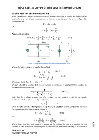
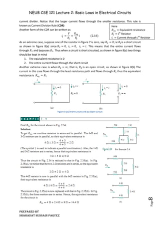
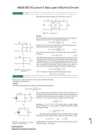
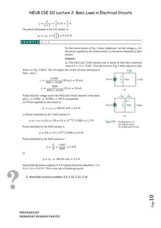
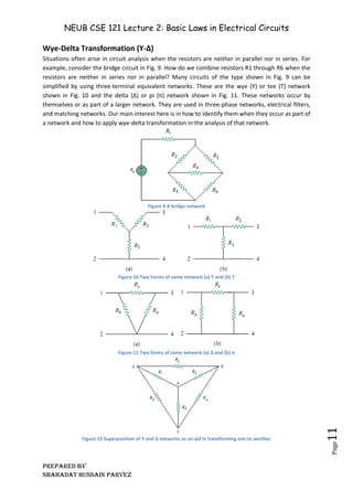
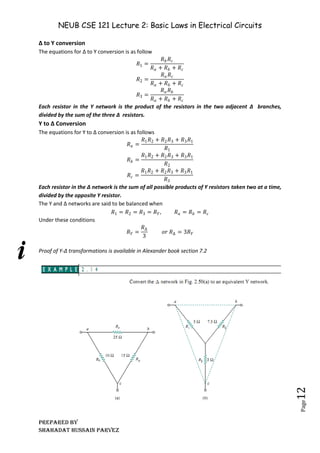
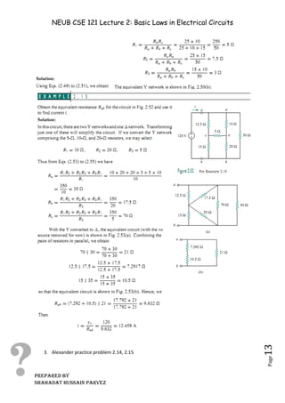
NEUB CSE 121 Lecture 2: Basic Laws in Electrical Circuits
Prepared BY
Shahadat Hussain Parvez
Page
1
Kirchhoff’s Laws
Ohm’s Law by itself is not sufficient to analyze circuits. Two of the important laws for analyzing
circuits came from German physicist Gustav Robert Kirchhoff in 1847. These laws are formally known
as Kirchhoff’s Current Law (KCL) and Kirchhoff’s Voltage Law (KVL).
Kirchhoff’s first law (KCL) is based on the law of conservation of charge, which requires that the
algebraic sum of charges within a system cannot change.
Kirchhoff’s current law (KCL) states that the algebraic sum of currents entering a node (or
a closed boundary) is zero.
Mathematically it can be written as
𝑖𝑛 = 0
𝑁
𝑛=1
(2.1)
Here N is the number of branches connected to the node and in is the nth
current entering (or
leaving) the node. By this law, currents entering a node may be regarded as positive, while currents
leaving the node may be taken as negative and current entering a node is considered as positive.
Figure 1 Current at a node illustrating KCL
Considering the node in figure 1, applying KCL gives
𝑖1 + −𝑖2 + 𝑖3 + 𝑖4 + −𝑖5 = 0
Or
𝑖1 + 𝑖3 + 𝑖4 = 𝑖2 + 𝑖5
So and alternative form of KCL can be stated as
The sum of the currents entering a node is equal to the sum of the currents leaving the node.
Note that KCL also applies to a closed boundary. This may be regarded as a generalized case,
because a node may be regarded as a closed surface shrunk to a point. In two dimensions, a closed
boundary is the same as a closed path. As typically illustrated in the circuit of Figure 2, the total
current entering the closed surface is equal to the total current leaving the surface.
Figure 2 Applying KCL to a closed boundary
NEUB CSE 121 Lecture 2: Basic Laws in Electrical Circuits
Prepared BY
Shahadat Hussain Parvez
Page
2
A simple application of KCL is combining current sources in par-allel. The combined current is the
algebraic sum of the current supplied by the individual sources. For example, the current sources
shown in figure 3(a) can be combined as in figure 3(b). The combined or equivalent current source
can be found by applying KCL to node a.
𝐼𝑇 + 𝐼2 = 𝐼1 + 𝐼3
Or
𝐼𝑇 = 𝐼1 − 𝐼2 + 𝐼3
A circuit cannot contain two different currents, 𝐼1 and 𝐼2, in series, unless 𝐼1 = 𝐼2; otherwise KCL
will be violated.
Figure 3 Current Sources in parallel (a) Original Circuit (b) equivalent Circuit
Kirchhoff’s second law (KVL) is based on the principle of conservation of energy:
Kirchhoff’s voltage law (KVL) states that the algebraic sum of all voltages around a closed
path (or loop) is zero.
KVL can be mathematically expressed as
𝑣𝑚 = 0
𝑀
𝑚=0
(2.2)
Here M is the number of voltages in the loop (or the number of branches in the loop) and vm is the
mth
voltage.
To illustrate KVL, consider the circuit in figure 4. The sign on each voltage is the polarity of the
terminal encountered first as we travel around the loop. We can start with any branch and go
around the loop either clockwise or counterclockwise. Suppose we start with the voltage source and
go clockwise around the loop as shown; then voltages would be – 𝑣1, +𝑣2, +𝑣3, −𝑣4, 𝑎𝑛𝑑 + 𝑣5, in
that order. For example, as we reach branch 3, the positive terminal is met first; hence we have+𝑣3.
For branch 4, we reach the negative terminal first; hence, − 𝑣4. Thus, KVL yields
−𝑣1 + 𝑣2 + 𝑣3 − 𝑣4 + 𝑣5 = 0
Or
𝑣1 + 𝑣4 = 𝑣2 + 𝑣3 + 𝑣5
This can be interpreted as
𝑆𝑢𝑚 𝑜𝑓 𝑣𝑜𝑙𝑡𝑎𝑔𝑒 𝑑𝑟𝑜𝑝𝑠 = 𝑆𝑢𝑚 𝑜𝑓 𝑣𝑜𝑙𝑡𝑎𝑔𝑒 𝑟𝑖𝑠𝑒𝑠 (2.3)
This is an alternative form of KVL. If we have travelled counterclockwise, we would have ended up
with same equation.
Figure 4 A single loop circuit illustrating KVL
NEUB CSE 121 Lecture 2: Basic Laws in Electrical Circuits
Prepared BY
Shahadat Hussain Parvez
Page
3
When voltage sources are connected in series, KVL can be applied to obtain the total voltage. The
combined voltage is the algebraic sum of the voltages of the individual sources. For example, for the
voltage sources shown in Fig. 5(a), the combined or equivalent voltage source in Fig. 5(b) is obtained
by applying KVL.
−𝑉𝑎𝑏 + 𝑉1 + 𝑉2 − 𝑉3 = 0
Or
𝑉𝑎𝑏 = 𝑉1 + 𝑉2 − 𝑉3
To avoid violating KVL, a circuit cannot contain two different voltages V1 and V2 in parallel
unless 𝑉1 = 𝑉2.
Figure 5 Voltage sources in series, (a) original circuit (b) equivalent circuit
NEUB CSE 121 Lecture 2: Basic Laws in Electrical Circuits
Prepared BY
Shahadat Hussain Parvez
Page
4
NEUB CSE 121 Lecture 2: Basic Laws in Electrical Circuits
Prepared BY
Shahadat Hussain Parvez
Page
5
1. Alexander Practice problems 2.5-2.8
NEUB CSE 121 Lecture 2: Basic Laws in Electrical Circuits
Prepared BY
Shahadat Hussain Parvez
Page
6
Series Resistors and Voltage Division
Combinations of resistors in series or parallel are so common, that it warrants some special
attention. The process of combining the resistors is facilitated by combining two of them at a time.
With this in mind, consider the single-loop circuit of Fig. 6(a). The two resistors are in series, since
the same current 𝑖 flows in both of them. Applying Ohm’s law to each of the resistors, we obtain
𝑉1 = 𝑖𝑅1, 𝑉2 = 𝑖𝑅2 (2.4)
If we apply KVL we get
−𝑉 + 𝑉1 + 𝑉2 = 0
Or
𝑉 = 𝑉1 + 𝑉2 = 𝑖 𝑅1 + 𝑅2 (2.5)
Therefore
𝑖 =
𝑉
𝑅1 + 𝑅2
(2.6)
We can also find the current using the equivalent circuit of figure 6(b)
𝑖 =
𝑉
𝑅𝑒𝑞
So we can imply that
𝑅𝑒𝑞 = 𝑅1 + 𝑅2 (2.7)
(a) (b)
Figure 6 (a)A series circuit with 2 resistors and (b) their equivalent circuit
In general it can be said as
The equivalent resistance of any number of resistors connected in series is the sum of the
individual resistances.
For N resistors in series then,
𝑹𝒆𝒒 = 𝑹𝟏 + 𝑹𝟐 + ⋯ + 𝑹𝑵 = 𝑹𝒏
𝑵
𝒏=𝟏
(𝟐. 𝟖)
To determine voltage across each resistor, we substitute equation 2.6 in equation 2.4 to get
𝑉1 =
𝑅1
𝑅1 + 𝑅2
𝑉, 𝑉2 =
𝑅2
𝑅1 + 𝑅2
𝑉 (2.9)
Notice that the source voltage v is divided among the resistors in direct proportion to their
resistances; the larger the resistance, the larger the voltage drop. This is called the principle of
voltage division, and the circuit in Fig. 6 is called a voltage divider. In general, if a voltage divider has
N resistors (R1,R2,...,RN ) in series with the source voltage v, the nth resistor (Rn) will have a voltage
drop of
𝑽𝒏 =
𝑹𝒏
𝑹𝟏 + 𝑹𝟐 + ⋯ + 𝑹𝑵
𝑽 (𝟐. 𝟏𝟎)
This rule is known as Voltage Division Rule (VDR)
NEUB CSE 121 Lecture 2: Basic Laws in Electrical Circuits
Prepared BY
Shahadat Hussain Parvez
Page
7
Parallel Resistors and Current Division
When two elements connect at a single node pair, they are said to be in parallel. Parallel-connected
circuit elements have the same voltage across their terminals. Consider the circuit in figure 7(a)
From Ohm’s law,
𝑉 = 𝑖1𝑅1 = 𝑖2𝑅2
Or
𝑖1 =
𝑉
𝑅1
, 𝑖2 =
𝑉
𝑅2
Applying KCL at node a
𝑖 = 𝑖1 + 𝑖2 =
𝑉
𝑅1
+
𝑉
𝑅2
= 𝑉
1
𝑅1
+
1
𝑅2
=
𝑉
𝑅𝑒𝑞
(2.11)
(a) (b)
Figure 7 (a) Two Resistors in parallel and (b) their equivalent circuit
Where 𝑅𝑒𝑞 is the resistance in parallel (Figure 7(b))
1
𝑅𝑒𝑞
=
1
𝑅1
+
1
𝑅2
(2.12)
𝑅𝑒𝑞 =
𝑅1𝑅2
𝑅1 + 𝑅2
=
1
1
𝑅1
+
1
𝑅2
(2.13)
We can see that if 𝑅1 = 𝑅2, 𝑅𝑒𝑞 =
𝑅1
2
We can extend the equation 2.13 for any number of resistances in parallel. SO the equation for
equivalent resistance become
𝑹𝒆𝒒 =
𝟏
𝟏
𝑹𝟏
+
𝟏
𝑹𝟐
+ ⋯ +
𝟏
𝑹𝑵
(𝟐. 𝟏𝟒)
Note that Req is always smaller than the resistance of the smallest resistor in the parallel
combination. If 𝑅1 = 𝑅2 = ··· = 𝑅𝑁 = 𝑅, then
𝑅𝑒𝑞 =
𝑅
𝑁
(2.15)
Given the total current 𝑖 entering node 𝑎 in Fig. 7, how do we obtain current i1 and i2? We know that
the equivalent resistor has the same voltage, or
𝑉 = 𝑖𝑅𝑒𝑞 =
𝑖 𝑅1𝑅2
𝑅1 + 𝑅2
(2.16)
So
𝑖1 =
𝑅2 𝑖
𝑅1 + 𝑅2
, 𝑖2 =
𝑅1 𝑖
𝑅1 + 𝑅2
(2.17)
Which shows that the total current 𝑖 is shared by the resistors in inverse proportion to their
resistances. This is known as the principle of current division, and the circuit in Fig. 7 is known as a
NEUB CSE 121 Lecture 2: Basic Laws in Electrical Circuits
Prepared BY
Shahadat Hussain Parvez
Page
8
current divider. Notice that the larger current flows through the smaller resistance. This rule is
known as Current Division Rule (CDR)
Another form of the CDR can be written as
𝑖𝑗 =
𝑉
𝑅𝑗
=
𝑅𝑒𝑞
𝑅𝑗
𝑖 (2.18)
As an extreme case, suppose one of the resistor in figure 7 is zero, say 𝑅2 = 0; ie 𝑅2is a short circuit
as shown in figure 8(a) since 𝑅2 = 0, 𝑖1 = 0, 𝑖1 = 𝑖. This means that the entire current flows
through 𝑅2 and bypasses 𝑅1. Thus when a circuit is short circuited, as shown in figure 8(a) two things
should be kept in mind
1. The equivalent resistance is 0
2. The entire current flows through the short circuit
Another extreme case is when 𝑅2 = ∞, that is, 𝑅2 is an open circuit, as shown in figure 8(b) The
current in this case flows through the least resistance path and flows through 𝑅1 thus the equivalent
resistance is 𝑅𝑒𝑞 = 𝑅1
Figure 8 (a) Short Circuit and (b) Open Circuit
Here
𝑅𝑒𝑞 = Equivalent resistance
𝑅𝑗 = Jth
Resistor
𝑖𝑗 = Current through Jth
Resistor
NEUB CSE 121 Lecture 2: Basic Laws in Electrical Circuits
Prepared BY
Shahadat Hussain Parvez
Page
9
NEUB CSE 121 Lecture 2: Basic Laws in Electrical Circuits
Prepared BY
Shahadat Hussain Parvez
Page
10
2. Alexander practice problem 2.9, 2.10, 2.12, 2.13
NEUB CSE 121 Lecture 2: Basic Laws in Electrical Circuits
Prepared BY
Shahadat Hussain Parvez
Page
11
Wye-Delta Transformation (Y-Δ)
Situations often arise in circuit analysis when the resistors are neither in parallel nor in series. For
example, consider the bridge circuit in Fig. 9. How do we combine resistors R1 through R6 when the
resistors are neither in series nor in parallel? Many circuits of the type shown in Fig. 9 can be
simplified by using three-terminal equivalent networks. These are the wye (Y) or tee (T) network
shown in Fig. 10 and the delta (Δ) or pi (π) network shown in Fig. 11. These networks occur by
themselves or as part of a larger network. They are used in three-phase networks, electrical filters,
and matching networks. Our main interest here is in how to identify them when they occur as part of
a network and how to apply wye-delta transformation in the analysis of that network.
Figure 9 A bridge network
Figure 10 Two Forms of same network (a) Y and (b) T
Figure 11 Two forms of same network (a) Δ and (b) π
Figure 12 Superposition of Y and Δ networks as an aid in transforming one to another
NEUB CSE 121 Lecture 2: Basic Laws in Electrical Circuits
Prepared BY
Shahadat Hussain Parvez
Page
12
Δ to Y conversion
The equations for Δ to Y conversion is as follow
𝑅1 =
𝑅𝑏𝑅𝑐
𝑅𝑎 + 𝑅𝑏 + 𝑅𝑐
𝑅2 =
𝑅𝑎 𝑅𝑐
𝑅𝑎 + 𝑅𝑏 + 𝑅𝑐
𝑅3 =
𝑅𝑎 𝑅𝑏
𝑅𝑎 + 𝑅𝑏 + 𝑅𝑐
Each resistor in the Y network is the product of the resistors in the two adjacent Δ branches,
divided by the sum of the three Δ resistors.
Y to Δ Conversion
The equations for Y to Δ conversion is as follows
𝑅𝑎 =
𝑅1𝑅2 + 𝑅2𝑅3 + 𝑅3𝑅1
𝑅1
𝑅𝑏 =
𝑅1𝑅2 + 𝑅2𝑅3 + 𝑅3𝑅1
𝑅2
𝑅𝑐 =
𝑅1𝑅2 + 𝑅2𝑅3 + 𝑅3𝑅1
𝑅3
Each resistor in the Δ network is the sum of all possible products of Y resistors taken two at a time,
divided by the opposite Y resistor.
The Y and Δ networks are said to be balanced when
𝑅1 = 𝑅2 = 𝑅3 = 𝑅𝑌, 𝑅𝑎 = 𝑅𝑏 = 𝑅𝑐
Under these conditions
𝑅𝑌 =
𝑅Δ
3
𝑜𝑟 𝑅Δ = 3𝑅𝑌
Proof of Y-Δ transformations is available in Alexander book section 7.2
NEUB CSE 121 Lecture 2: Basic Laws in Electrical Circuits
Prepared BY
Shahadat Hussain Parvez
Page
13
3. Alexander practice problem 2.14, 2.15

neub-cse-121-lec-2.pdf Basic-Electric-and-Circuit

  • 1.
    NEUB CSE 121Lecture 2: Basic Laws in Electrical Circuits Prepared BY Shahadat Hussain Parvez Page 1 Kirchhoff’s Laws Ohm’s Law by itself is not sufficient to analyze circuits. Two of the important laws for analyzing circuits came from German physicist Gustav Robert Kirchhoff in 1847. These laws are formally known as Kirchhoff’s Current Law (KCL) and Kirchhoff’s Voltage Law (KVL). Kirchhoff’s first law (KCL) is based on the law of conservation of charge, which requires that the algebraic sum of charges within a system cannot change. Kirchhoff’s current law (KCL) states that the algebraic sum of currents entering a node (or a closed boundary) is zero. Mathematically it can be written as 𝑖𝑛 = 0 𝑁 𝑛=1 (2.1) Here N is the number of branches connected to the node and in is the nth current entering (or leaving) the node. By this law, currents entering a node may be regarded as positive, while currents leaving the node may be taken as negative and current entering a node is considered as positive. Figure 1 Current at a node illustrating KCL Considering the node in figure 1, applying KCL gives 𝑖1 + −𝑖2 + 𝑖3 + 𝑖4 + −𝑖5 = 0 Or 𝑖1 + 𝑖3 + 𝑖4 = 𝑖2 + 𝑖5 So and alternative form of KCL can be stated as The sum of the currents entering a node is equal to the sum of the currents leaving the node. Note that KCL also applies to a closed boundary. This may be regarded as a generalized case, because a node may be regarded as a closed surface shrunk to a point. In two dimensions, a closed boundary is the same as a closed path. As typically illustrated in the circuit of Figure 2, the total current entering the closed surface is equal to the total current leaving the surface. Figure 2 Applying KCL to a closed boundary
  • 2.
    NEUB CSE 121Lecture 2: Basic Laws in Electrical Circuits Prepared BY Shahadat Hussain Parvez Page 2 A simple application of KCL is combining current sources in par-allel. The combined current is the algebraic sum of the current supplied by the individual sources. For example, the current sources shown in figure 3(a) can be combined as in figure 3(b). The combined or equivalent current source can be found by applying KCL to node a. 𝐼𝑇 + 𝐼2 = 𝐼1 + 𝐼3 Or 𝐼𝑇 = 𝐼1 − 𝐼2 + 𝐼3 A circuit cannot contain two different currents, 𝐼1 and 𝐼2, in series, unless 𝐼1 = 𝐼2; otherwise KCL will be violated. Figure 3 Current Sources in parallel (a) Original Circuit (b) equivalent Circuit Kirchhoff’s second law (KVL) is based on the principle of conservation of energy: Kirchhoff’s voltage law (KVL) states that the algebraic sum of all voltages around a closed path (or loop) is zero. KVL can be mathematically expressed as 𝑣𝑚 = 0 𝑀 𝑚=0 (2.2) Here M is the number of voltages in the loop (or the number of branches in the loop) and vm is the mth voltage. To illustrate KVL, consider the circuit in figure 4. The sign on each voltage is the polarity of the terminal encountered first as we travel around the loop. We can start with any branch and go around the loop either clockwise or counterclockwise. Suppose we start with the voltage source and go clockwise around the loop as shown; then voltages would be – 𝑣1, +𝑣2, +𝑣3, −𝑣4, 𝑎𝑛𝑑 + 𝑣5, in that order. For example, as we reach branch 3, the positive terminal is met first; hence we have+𝑣3. For branch 4, we reach the negative terminal first; hence, − 𝑣4. Thus, KVL yields −𝑣1 + 𝑣2 + 𝑣3 − 𝑣4 + 𝑣5 = 0 Or 𝑣1 + 𝑣4 = 𝑣2 + 𝑣3 + 𝑣5 This can be interpreted as 𝑆𝑢𝑚 𝑜𝑓 𝑣𝑜𝑙𝑡𝑎𝑔𝑒 𝑑𝑟𝑜𝑝𝑠 = 𝑆𝑢𝑚 𝑜𝑓 𝑣𝑜𝑙𝑡𝑎𝑔𝑒 𝑟𝑖𝑠𝑒𝑠 (2.3) This is an alternative form of KVL. If we have travelled counterclockwise, we would have ended up with same equation. Figure 4 A single loop circuit illustrating KVL
  • 3.
    NEUB CSE 121Lecture 2: Basic Laws in Electrical Circuits Prepared BY Shahadat Hussain Parvez Page 3 When voltage sources are connected in series, KVL can be applied to obtain the total voltage. The combined voltage is the algebraic sum of the voltages of the individual sources. For example, for the voltage sources shown in Fig. 5(a), the combined or equivalent voltage source in Fig. 5(b) is obtained by applying KVL. −𝑉𝑎𝑏 + 𝑉1 + 𝑉2 − 𝑉3 = 0 Or 𝑉𝑎𝑏 = 𝑉1 + 𝑉2 − 𝑉3 To avoid violating KVL, a circuit cannot contain two different voltages V1 and V2 in parallel unless 𝑉1 = 𝑉2. Figure 5 Voltage sources in series, (a) original circuit (b) equivalent circuit
  • 4.
    NEUB CSE 121Lecture 2: Basic Laws in Electrical Circuits Prepared BY Shahadat Hussain Parvez Page 4
  • 5.
    NEUB CSE 121Lecture 2: Basic Laws in Electrical Circuits Prepared BY Shahadat Hussain Parvez Page 5 1. Alexander Practice problems 2.5-2.8
  • 6.
    NEUB CSE 121Lecture 2: Basic Laws in Electrical Circuits Prepared BY Shahadat Hussain Parvez Page 6 Series Resistors and Voltage Division Combinations of resistors in series or parallel are so common, that it warrants some special attention. The process of combining the resistors is facilitated by combining two of them at a time. With this in mind, consider the single-loop circuit of Fig. 6(a). The two resistors are in series, since the same current 𝑖 flows in both of them. Applying Ohm’s law to each of the resistors, we obtain 𝑉1 = 𝑖𝑅1, 𝑉2 = 𝑖𝑅2 (2.4) If we apply KVL we get −𝑉 + 𝑉1 + 𝑉2 = 0 Or 𝑉 = 𝑉1 + 𝑉2 = 𝑖 𝑅1 + 𝑅2 (2.5) Therefore 𝑖 = 𝑉 𝑅1 + 𝑅2 (2.6) We can also find the current using the equivalent circuit of figure 6(b) 𝑖 = 𝑉 𝑅𝑒𝑞 So we can imply that 𝑅𝑒𝑞 = 𝑅1 + 𝑅2 (2.7) (a) (b) Figure 6 (a)A series circuit with 2 resistors and (b) their equivalent circuit In general it can be said as The equivalent resistance of any number of resistors connected in series is the sum of the individual resistances. For N resistors in series then, 𝑹𝒆𝒒 = 𝑹𝟏 + 𝑹𝟐 + ⋯ + 𝑹𝑵 = 𝑹𝒏 𝑵 𝒏=𝟏 (𝟐. 𝟖) To determine voltage across each resistor, we substitute equation 2.6 in equation 2.4 to get 𝑉1 = 𝑅1 𝑅1 + 𝑅2 𝑉, 𝑉2 = 𝑅2 𝑅1 + 𝑅2 𝑉 (2.9) Notice that the source voltage v is divided among the resistors in direct proportion to their resistances; the larger the resistance, the larger the voltage drop. This is called the principle of voltage division, and the circuit in Fig. 6 is called a voltage divider. In general, if a voltage divider has N resistors (R1,R2,...,RN ) in series with the source voltage v, the nth resistor (Rn) will have a voltage drop of 𝑽𝒏 = 𝑹𝒏 𝑹𝟏 + 𝑹𝟐 + ⋯ + 𝑹𝑵 𝑽 (𝟐. 𝟏𝟎) This rule is known as Voltage Division Rule (VDR)
  • 7.
    NEUB CSE 121Lecture 2: Basic Laws in Electrical Circuits Prepared BY Shahadat Hussain Parvez Page 7 Parallel Resistors and Current Division When two elements connect at a single node pair, they are said to be in parallel. Parallel-connected circuit elements have the same voltage across their terminals. Consider the circuit in figure 7(a) From Ohm’s law, 𝑉 = 𝑖1𝑅1 = 𝑖2𝑅2 Or 𝑖1 = 𝑉 𝑅1 , 𝑖2 = 𝑉 𝑅2 Applying KCL at node a 𝑖 = 𝑖1 + 𝑖2 = 𝑉 𝑅1 + 𝑉 𝑅2 = 𝑉 1 𝑅1 + 1 𝑅2 = 𝑉 𝑅𝑒𝑞 (2.11) (a) (b) Figure 7 (a) Two Resistors in parallel and (b) their equivalent circuit Where 𝑅𝑒𝑞 is the resistance in parallel (Figure 7(b)) 1 𝑅𝑒𝑞 = 1 𝑅1 + 1 𝑅2 (2.12) 𝑅𝑒𝑞 = 𝑅1𝑅2 𝑅1 + 𝑅2 = 1 1 𝑅1 + 1 𝑅2 (2.13) We can see that if 𝑅1 = 𝑅2, 𝑅𝑒𝑞 = 𝑅1 2 We can extend the equation 2.13 for any number of resistances in parallel. SO the equation for equivalent resistance become 𝑹𝒆𝒒 = 𝟏 𝟏 𝑹𝟏 + 𝟏 𝑹𝟐 + ⋯ + 𝟏 𝑹𝑵 (𝟐. 𝟏𝟒) Note that Req is always smaller than the resistance of the smallest resistor in the parallel combination. If 𝑅1 = 𝑅2 = ··· = 𝑅𝑁 = 𝑅, then 𝑅𝑒𝑞 = 𝑅 𝑁 (2.15) Given the total current 𝑖 entering node 𝑎 in Fig. 7, how do we obtain current i1 and i2? We know that the equivalent resistor has the same voltage, or 𝑉 = 𝑖𝑅𝑒𝑞 = 𝑖 𝑅1𝑅2 𝑅1 + 𝑅2 (2.16) So 𝑖1 = 𝑅2 𝑖 𝑅1 + 𝑅2 , 𝑖2 = 𝑅1 𝑖 𝑅1 + 𝑅2 (2.17) Which shows that the total current 𝑖 is shared by the resistors in inverse proportion to their resistances. This is known as the principle of current division, and the circuit in Fig. 7 is known as a
  • 8.
    NEUB CSE 121Lecture 2: Basic Laws in Electrical Circuits Prepared BY Shahadat Hussain Parvez Page 8 current divider. Notice that the larger current flows through the smaller resistance. This rule is known as Current Division Rule (CDR) Another form of the CDR can be written as 𝑖𝑗 = 𝑉 𝑅𝑗 = 𝑅𝑒𝑞 𝑅𝑗 𝑖 (2.18) As an extreme case, suppose one of the resistor in figure 7 is zero, say 𝑅2 = 0; ie 𝑅2is a short circuit as shown in figure 8(a) since 𝑅2 = 0, 𝑖1 = 0, 𝑖1 = 𝑖. This means that the entire current flows through 𝑅2 and bypasses 𝑅1. Thus when a circuit is short circuited, as shown in figure 8(a) two things should be kept in mind 1. The equivalent resistance is 0 2. The entire current flows through the short circuit Another extreme case is when 𝑅2 = ∞, that is, 𝑅2 is an open circuit, as shown in figure 8(b) The current in this case flows through the least resistance path and flows through 𝑅1 thus the equivalent resistance is 𝑅𝑒𝑞 = 𝑅1 Figure 8 (a) Short Circuit and (b) Open Circuit Here 𝑅𝑒𝑞 = Equivalent resistance 𝑅𝑗 = Jth Resistor 𝑖𝑗 = Current through Jth Resistor
  • 9.
    NEUB CSE 121Lecture 2: Basic Laws in Electrical Circuits Prepared BY Shahadat Hussain Parvez Page 9
  • 10.
    NEUB CSE 121Lecture 2: Basic Laws in Electrical Circuits Prepared BY Shahadat Hussain Parvez Page 10 2. Alexander practice problem 2.9, 2.10, 2.12, 2.13
  • 11.
    NEUB CSE 121Lecture 2: Basic Laws in Electrical Circuits Prepared BY Shahadat Hussain Parvez Page 11 Wye-Delta Transformation (Y-Δ) Situations often arise in circuit analysis when the resistors are neither in parallel nor in series. For example, consider the bridge circuit in Fig. 9. How do we combine resistors R1 through R6 when the resistors are neither in series nor in parallel? Many circuits of the type shown in Fig. 9 can be simplified by using three-terminal equivalent networks. These are the wye (Y) or tee (T) network shown in Fig. 10 and the delta (Δ) or pi (π) network shown in Fig. 11. These networks occur by themselves or as part of a larger network. They are used in three-phase networks, electrical filters, and matching networks. Our main interest here is in how to identify them when they occur as part of a network and how to apply wye-delta transformation in the analysis of that network. Figure 9 A bridge network Figure 10 Two Forms of same network (a) Y and (b) T Figure 11 Two forms of same network (a) Δ and (b) π Figure 12 Superposition of Y and Δ networks as an aid in transforming one to another
  • 12.
    NEUB CSE 121Lecture 2: Basic Laws in Electrical Circuits Prepared BY Shahadat Hussain Parvez Page 12 Δ to Y conversion The equations for Δ to Y conversion is as follow 𝑅1 = 𝑅𝑏𝑅𝑐 𝑅𝑎 + 𝑅𝑏 + 𝑅𝑐 𝑅2 = 𝑅𝑎 𝑅𝑐 𝑅𝑎 + 𝑅𝑏 + 𝑅𝑐 𝑅3 = 𝑅𝑎 𝑅𝑏 𝑅𝑎 + 𝑅𝑏 + 𝑅𝑐 Each resistor in the Y network is the product of the resistors in the two adjacent Δ branches, divided by the sum of the three Δ resistors. Y to Δ Conversion The equations for Y to Δ conversion is as follows 𝑅𝑎 = 𝑅1𝑅2 + 𝑅2𝑅3 + 𝑅3𝑅1 𝑅1 𝑅𝑏 = 𝑅1𝑅2 + 𝑅2𝑅3 + 𝑅3𝑅1 𝑅2 𝑅𝑐 = 𝑅1𝑅2 + 𝑅2𝑅3 + 𝑅3𝑅1 𝑅3 Each resistor in the Δ network is the sum of all possible products of Y resistors taken two at a time, divided by the opposite Y resistor. The Y and Δ networks are said to be balanced when 𝑅1 = 𝑅2 = 𝑅3 = 𝑅𝑌, 𝑅𝑎 = 𝑅𝑏 = 𝑅𝑐 Under these conditions 𝑅𝑌 = 𝑅Δ 3 𝑜𝑟 𝑅Δ = 3𝑅𝑌 Proof of Y-Δ transformations is available in Alexander book section 7.2
  • 13.
    NEUB CSE 121Lecture 2: Basic Laws in Electrical Circuits Prepared BY Shahadat Hussain Parvez Page 13 3. Alexander practice problem 2.14, 2.15