DC Motor Control

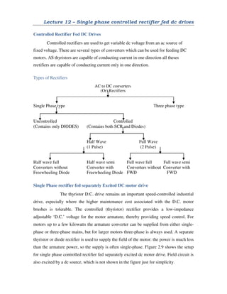
1. Lecture 12 – Single phase controlled rectifier fed dc drives
Controlled Rectifier Fed DC Drives
Controlled rectifiers are used to get variable dc voltage from an ac source of
fixed voltage. There are several types of converters which can be used for feeding DC
motors. AS thyristors are capable of conducting current in one direction all theses
rectifiers are capable of conducting current only in one direction.
Types of Rectifiers
AC to DC converters
(Or) Rectifiers
Single Phase type Three phase type
Uncontrolled Controlled
(Contains only DIODES) (Contains both SCR and Diodes)
Half Wave Full Wave
(1 Pulse) (2 Pulse)
Half wave full Half wave semi Full wave full Full wave semi
Converters without Converter with Converters without Converter with
Freewheeling Diode Freewheeling Diode FWD FWD
Single Phase rectifier fed separately Excited DC motor drive
The thyristor D.C. drive remains an important speed-controlled industrial
drive, especially where the higher maintenance cost associated with the D.C. motor
brushes is tolerable. The controlled (thyristor) rectifier provides a low-impedance
adjustable ‘D.C.’ voltage for the motor armature, thereby providing speed control. For
motors up to a few kilowatts the armature converter can be supplied from either single-
phase or three-phase mains, but for larger motors three-phase is always used. A separate
thyristor or diode rectifier is used to supply the field of the motor: the power is much less
than the armature power, so the supply is often single-phase. Figure 2.9 shows the setup
for single phase controlled rectifier fed separately excited dc motor drive. Field circuit is
also excited by a dc source, which is not shown in the figure just for simplicity.

2. The motor terminal voltage waveform and current waveform for the dominant
discontinuous and continuous conduction modes are show
(b).Thyristors TA and TB are gated at
ifVm sinα > E . Thyristors TA
and TB
’
are given gate pulses from
continuously the motor is said to operate in discontinuous conduction mode. When
current flows continuously, the conduction is said to be continuous. In discontinuous
modes, the current starts flowing with the turn on t
gets connected to the source and its terminal voltage equals V
At some angle β known as extinction angle, load current decays to zero. Here
π . As TA and TB are reversed biased after
ωt = β when Ia=0. From
from V sin β to E .At ωt =
m
up again as before and load voltage V
2.10(a). At (π + β ), Ia falls to zero, V
conducts.
Fig: Single phase rectifier
The motor terminal voltage waveform and current waveform for the dominant
and continuous conduction modes are shown in the figure (a)
are gated at ωt = α .The SCR’s will get turned on only
A and TB are given gate pulses from α to π and thyristors T
are given gate pulses from (π +α ) to 2π . When armature current does not flow
continuously the motor is said to operate in discontinuous conduction mode. When
current flows continuously, the conduction is said to be continuous. In discontinuous
modes, the current starts flowing with the turn on thyristors TA and TB atω
gets connected to the source and its terminal voltage equals Vs.
known as extinction angle, load current decays to zero. Here
are reversed biased afterωt = π , this pair is commutated at
=0. From β to (π +α ), no SCR’s conducts, the terminal voltage jumps
β as pair TA
’
and TB
’
is triggered, load current starts to build
up again as before and load voltage Va follows Vs waveform as shown in the figure
falls to zero, Va changes from Vm sin(π + β ) to E as no SCR
The motor terminal voltage waveform and current waveform for the dominant
.The SCR’s will get turned on only
and thyristors TA
’
When armature current does not flow
continuously the motor is said to operate in discontinuous conduction mode. When
current flows continuously, the conduction is said to be continuous. In discontinuous
ωt = α . Motor
known as extinction angle, load current decays to zero. Here β >
ed at
, no SCR’s conducts, the terminal voltage jumps
is triggered, load current starts to build
waveform as shown in the figure
to E as no SCR

3. Fig 2.10 (a) Discontinuous Conduction Mode Waveforms
In continuous conduction mode, during the positive half cycle thyristiors T
are forward biased. Atωt = α
Vm sinα immediately appears across thyristors T
turned off by natural commutation. At
are triggered causing turn off of T
Fig 2.10 (a) Discontinuous Conduction Mode Waveforms
In continuous conduction mode, during the positive half cycle thyristiors T
α , TA and TB are turned ON. As a result, supply voltage
immediately appears across thyristors TA
’
and TB
’
as a reverse bias, they are
turned off by natural commutation. At ωt = (π + α ) forward biased SCR’s T
are triggered causing turn off of TA and TB.
Fig 2.10 (a) Discontinuous Conduction Mode Waveforms
In continuous conduction mode, during the positive half cycle thyristiors TA and TB
are turned ON. As a result, supply voltage
as a reverse bias, they are
forward biased SCR’s TA
’
and TB
’

4. Fig (b) Continuous Conduction Waveforms
Discontinuous Conduction:
The drive operates in two intervals.
a) Conduction period(α ≤
Also(π + α ) ≤ ωt ≤ (
b) Idle period β ≤ ωt ≤ (π
Drive operation is described
(b) Continuous Conduction Waveforms
The drive operates in two intervals.
≤ ωt ≤ β ), TA and TB conduct and V0=Vs
(π + β ), TA
’
and TB
’
conduct and V0=Vs.
π +α ) when Ia=0 and Va=E.
Drive operation is described by the following equations
s.

5. V = R i + L dia + E = V sinωt for α ≤ ωt ≤ β (2.23)
a a a a dt m
for β ≤ ωt ≤ (π +α )
Va = E and ia = 0 (2.24)
From (2.23) we get
dia =Ra i = Vm sinωt − E (2.25)
dt L a L
a a
In order to get the speed torque characteristics for different values of α of the controlled
rectifier fed separately excited DC motor, it is necessary to solve the above equation
(2.25). So solving the above equation involves two mathematical steps, one is to evaluate
the complementary solution of the equation (2.25) and particular integral solution of the
equation (2.25).
Solution to Complementary Function:
The complementary function of equation (2.25) is
di
a
+
R
a
ia =0
dt La
d Ra
+ i = 0
a
dt
L
a
d + m1 = 0where
(i.e.)The above equation is of the form
dx
(2.26)
d
represents
d
and m1 dx
dt
R
a d + m1 = 0is D=-m1. Therefore the roots of the
represents . Roots of the equation
La dx
Ra d + m1 = 0
equation 2.26 is m = - . If the roots of the equation is real than the
L
a dx
complementary function is given by, C.F = C1e
mx
therefore complementary function of
the equation (2.26) is given by,
−
R
a t
C.F = C e
L
a (2.27)
1
We know that for an RL circuit Z=R+jXL
∴tanφ =
ωLa
R
a
⇒ cotφ =
Ra
ωLa
⇒ ω cotφ =
Ra
La

6. Substituting the above relation in equation (2.27) we get,
C.F. = C e−ωt cotφ (2.28)
1
Therefore the complementary function solution of the equation (2.25) is as given in
equation (2.28). The next step is to find the particular integral solution of equation (2.25).
In the expression (2.25) there are two Particular Integrals they are
E
La
Let us fine the solution of particular integrals one by one.
Solution to Particular Integral 1:
If X is sin (aX) or cos (aX) then the solution of P.I can be found out by
PI=
1
sin aX and replace D
2
by –a
2
f (D)
Therefore P.I 1 can be written as,
= 1
PI1
D +
R
a
La
V
m d
sinωt Where D = and a=ω
La dt
Multiplying and dividing by the conjugate in the above expression we get,
R
D − a
V
L
PI1 = a m
sinωt
R R L
D + a
D − a a
L
a
L
a
R
D − a
sinωt
Vm La
=
La
2
R
D
2
− a
L
a
replace D
2
= −ω
2
in the above expression we get,
La
and the other one is P.I2= −
P.I1=
V
m
sinωt

7. R
D − a
sinωt
Vm
∴ PI1 =
L
a
L
a
2
−ω2
− Ra
2
La
R
a
Dsinωt − sinωt
=
V
m
L
a
La
−
ω2
La
2
− Ra2
2
La
R
a
cosωt.ω − sinωt
=
V
m
L
a
since D =
La
−
ω2
La
2
− Ra2
2
La
d
dt
Vm cosωt.ωLa − Ra sinωt
=
La
2
−
ω2
La
2
− Ra
2
La
2
ωLa cosωt − Ra sinωt
(2.29)
= -Vm
(ω 2
La
2
+Ra
2
)
Now let us consider a triangle as shown in the figure 2.11
(ωLa )2
+ Ra 2
ωLa
φ
Ra
Fig 2.11
From the above figure cosφ =
R
a
and sin φ =
ωLa
(ωLa )2
+ Ra 2 (ωLa )2
+ Ra 2
Substituting the above two relation in equation (2.29) we get

8. Vm ωLa Ra
= − cosωt − sinωt
2 2 2 2 2 2
(ωLa ) (ωLa ) + Ra (ωLa ) + Ra
+R
a
= −
Vm
[sinφ.cosωt − cosφ.sinωt]
Z
=
Vm
[cosφ.sinωt − sinφ.cosωt]
Z
=
Vm
[sin(ωt − φ )]
Z
Solution to Particular Integral 2:
1 E
PI2 = −
R L
D + a a
L
a
1 E
= − e
0ia
Q D = 0
R L
a a
D +
L
a
1 E E
= − = −
Ra Ra
L
a
L
a
(2.30)
(2.31)
So combining equations (2.28), (2.30) and (2.31) gives the solution of equation (2.25)
i (ωt) = Vm sin(ωt −φ )− E +C1e−ωtcotφ
a
Z Ra
Where Z = Ra
2
+ (ωLa )2
φ = tan−1 ωL
a
R
a
constant C1 can be evaluated by using the initial condition ia (α ) = 0 and ωt = 0
V m
sin(α − φ )−
E
C1 = − eα cotφ
Z
R
a
Substituting (2.35) in (2.32) we get,
(2.32)
(2.33)
(2.34)
(2.35)

9. ia =
Vm
sin(ωt − φ )−
E
−
V m
sin(α − φ )−
E −(ωt−α )cotφ
e
Ra
Z Z R
a
since ia ( β ) = 0 from (2.36)
Vm
sin( β − φ )−
E V m
sin(α − φ )−
E
ia (β ) = − e−( β −α )cotφ
Ra
Z Z
R
a
β can be evaluated by iterative solution of (2.37)
Va = E + Ia Ra
From discontinuous waveforms
1
β π +α
V = ∫V sinωt d(ωt) + ∫ E d(ωt)
m
a
π α β
= Vm [cosα − cos β ]+(π + α − β )E [Q ∫sinθdθ = cosθ ]
π π
From equations (2.38) and (2.39)
Vm β − α
[cosα − cos β ]− Ia Ra = E
π π
Substituting (2.6) and (2.8) in (2.40)
Vm
[cosα − cos β ]−
T β − α
[Where K = Kaφ]
Ra = Kωm
π K π
ωm
β − α
=
V
m
[cos α − cos β ]−
T
Ra
π Kπ K
2
ωm =
V
[cosα − cos β ]−
T π
m
.Ra .
K(β − α ) K2 (β − α )
(2.36)
(2.37)
(2.38)
(2.39)
(2.40)
ωm =
Vm cosα − cos β
−
Ra π
T (2.41)
(β − α ) K
2
( β − α )
K
For a givenα , there is a particular speed ωmc when β = π + α , indicating that atωmc , the
mode of operation changes from discontinuous to continuous.ωmc is called as critical
speed. Substituting β = π + α in equation (2.37) we get,
Vm sin(π + α − φ )−
E V m sin(α − φ )−
E
− e−(π +α −α )cotφ (2.42)
Z Ra Z
R
a
− Vm sin(α − φ )− E − Vm sin(α − φ )e−π cotφ + E e−π cotφ =0 (2.43)
Z Ra Z Ra

10. −
Vm
sin(α − φ )[1+ e−π cotφ ]+
E
[e−π cotφ −1]= 0
Z Ra
E
[e −π cotφ −1]= Vm sin(α − φ )[1 + e−π cotφ ]
Ra Z
R a
1 +e−π cotφ
E = V sin(α − φ )
m −π cotφ
Z
e
−1
E = Kωmc
Ra
1 +e−π cotφ
ω = V sin(α − φ )
mc m −π cotφ
KZ
e
−1
Continuous Conduction Mode
For continuous conduction, average output voltage is given by,
π +α
Va =
1
∫Vm sinωtd(ωt)
π
α
V = 2Vm cosα
a
π
ω = 2Vm cosα − Ra T
M K2
πK
(2.44)
(2.45)
(2.46)
(2.47)
(2.48)
Fig (c)