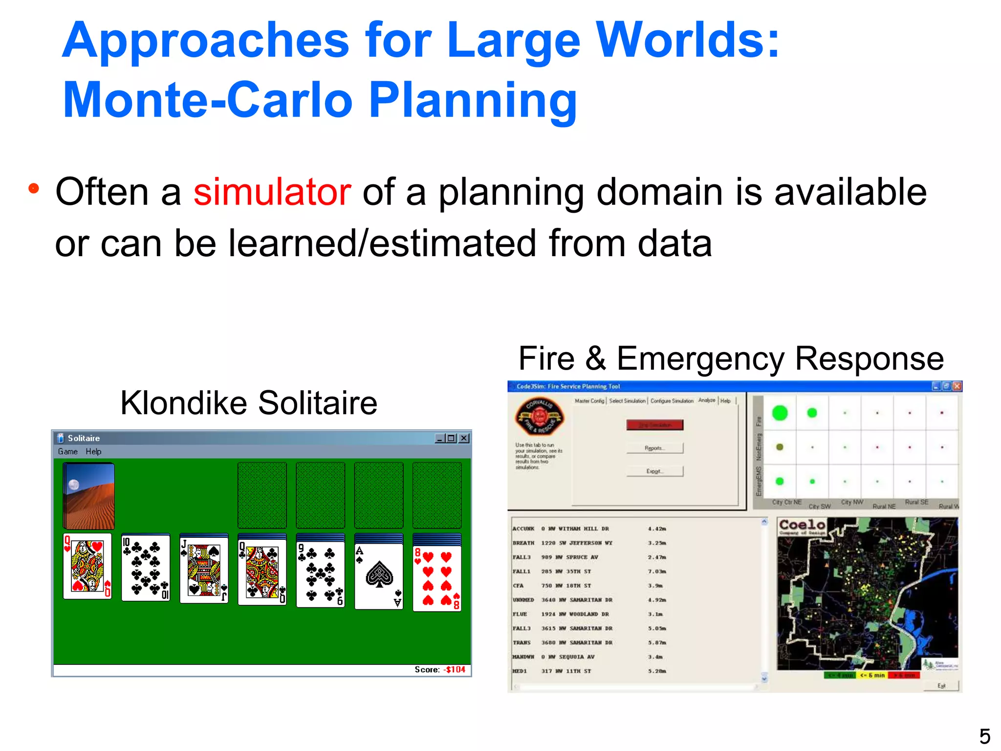
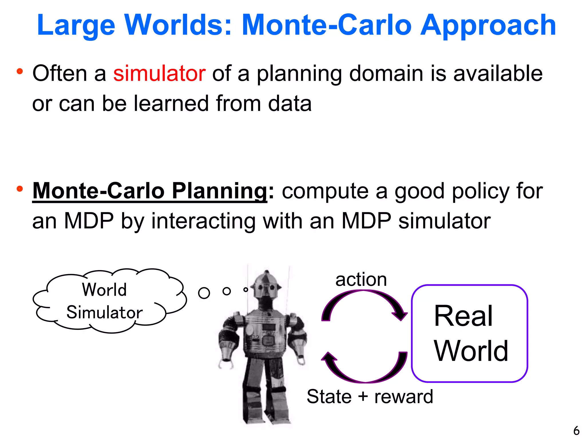
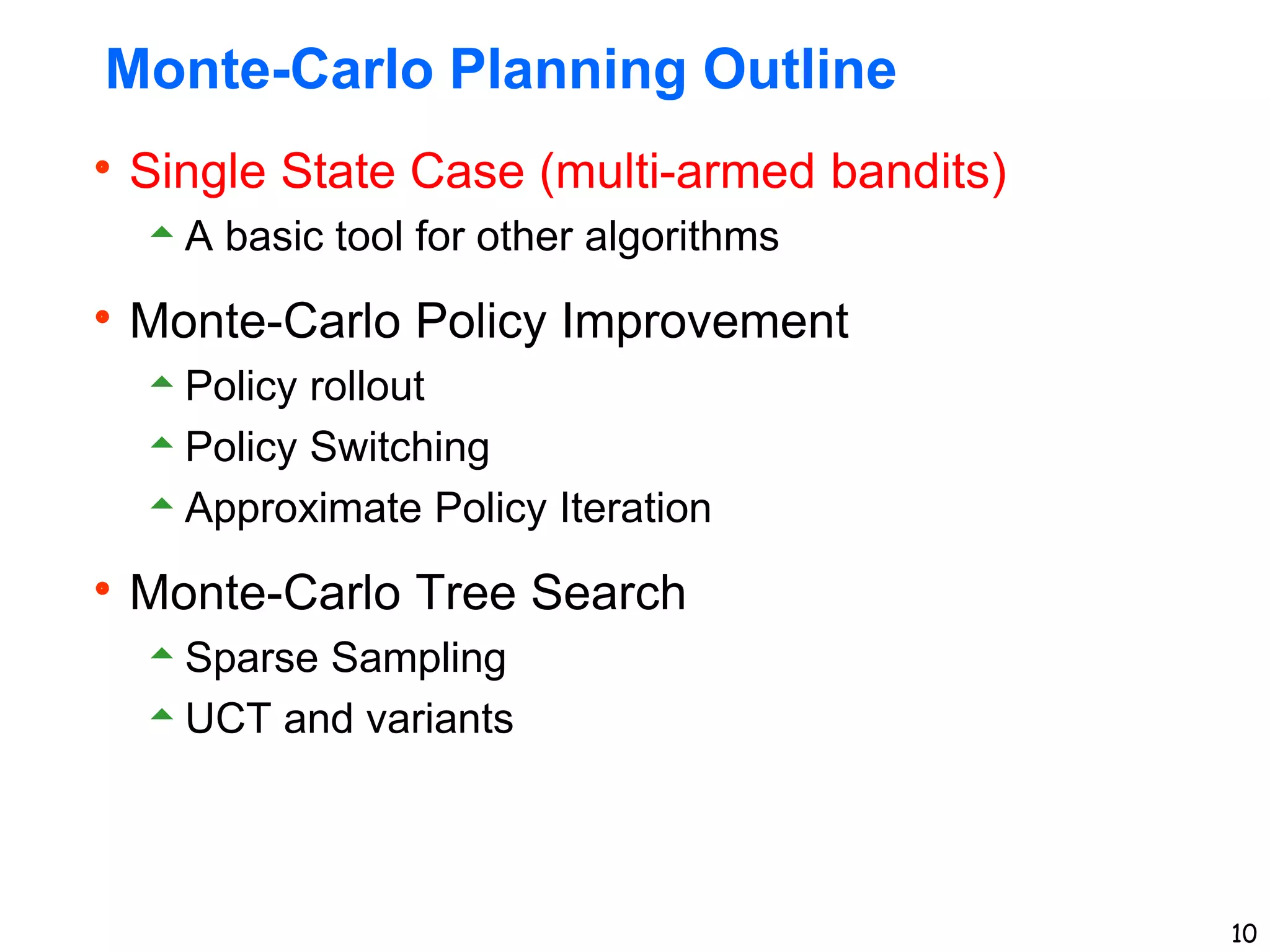
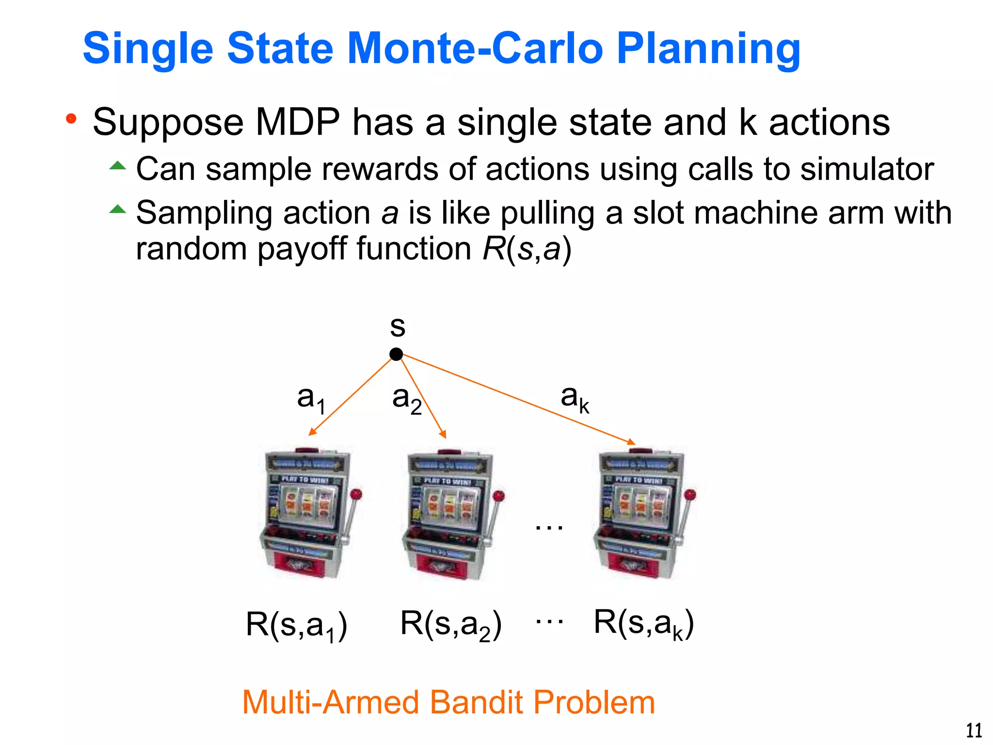
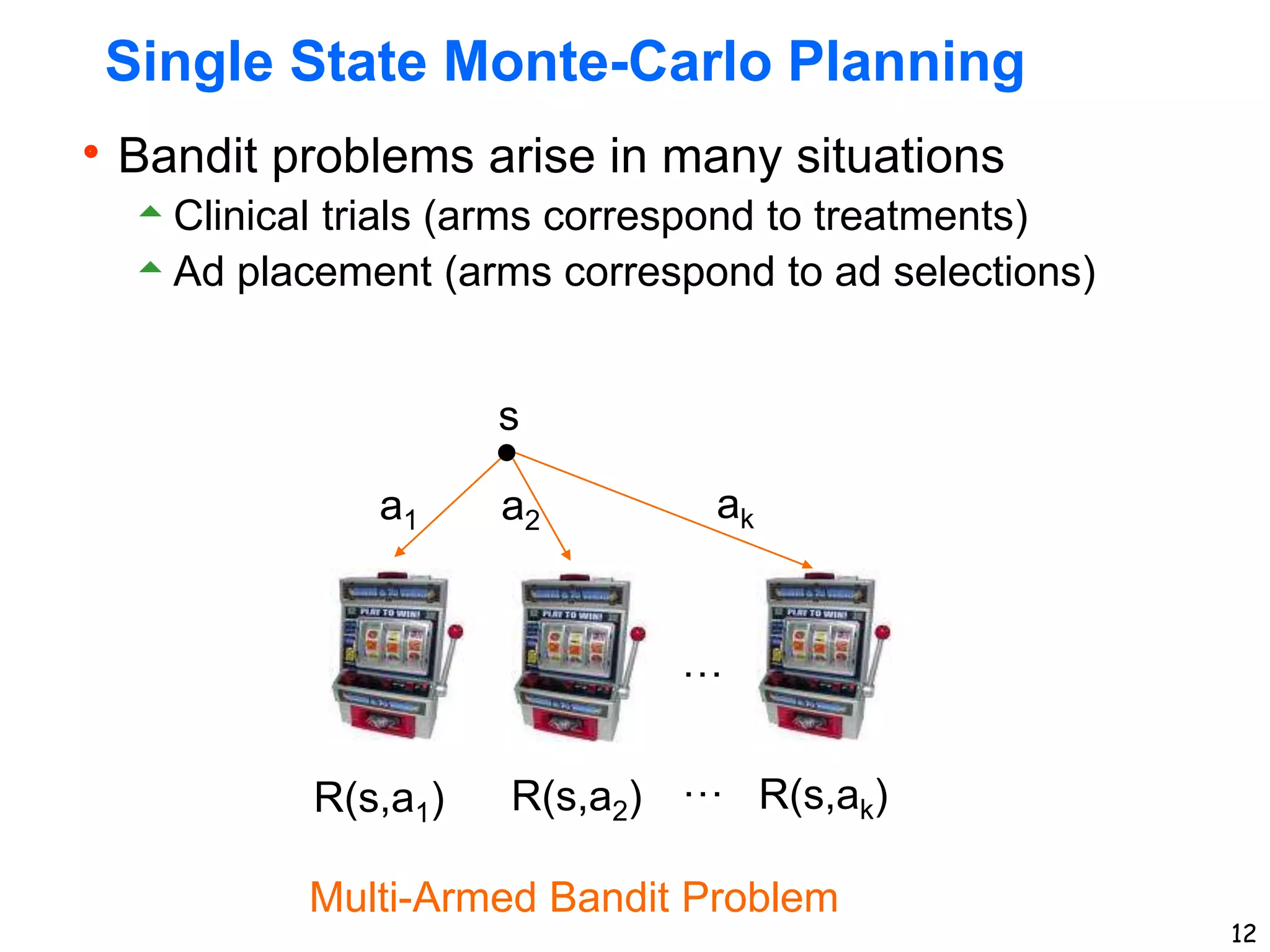
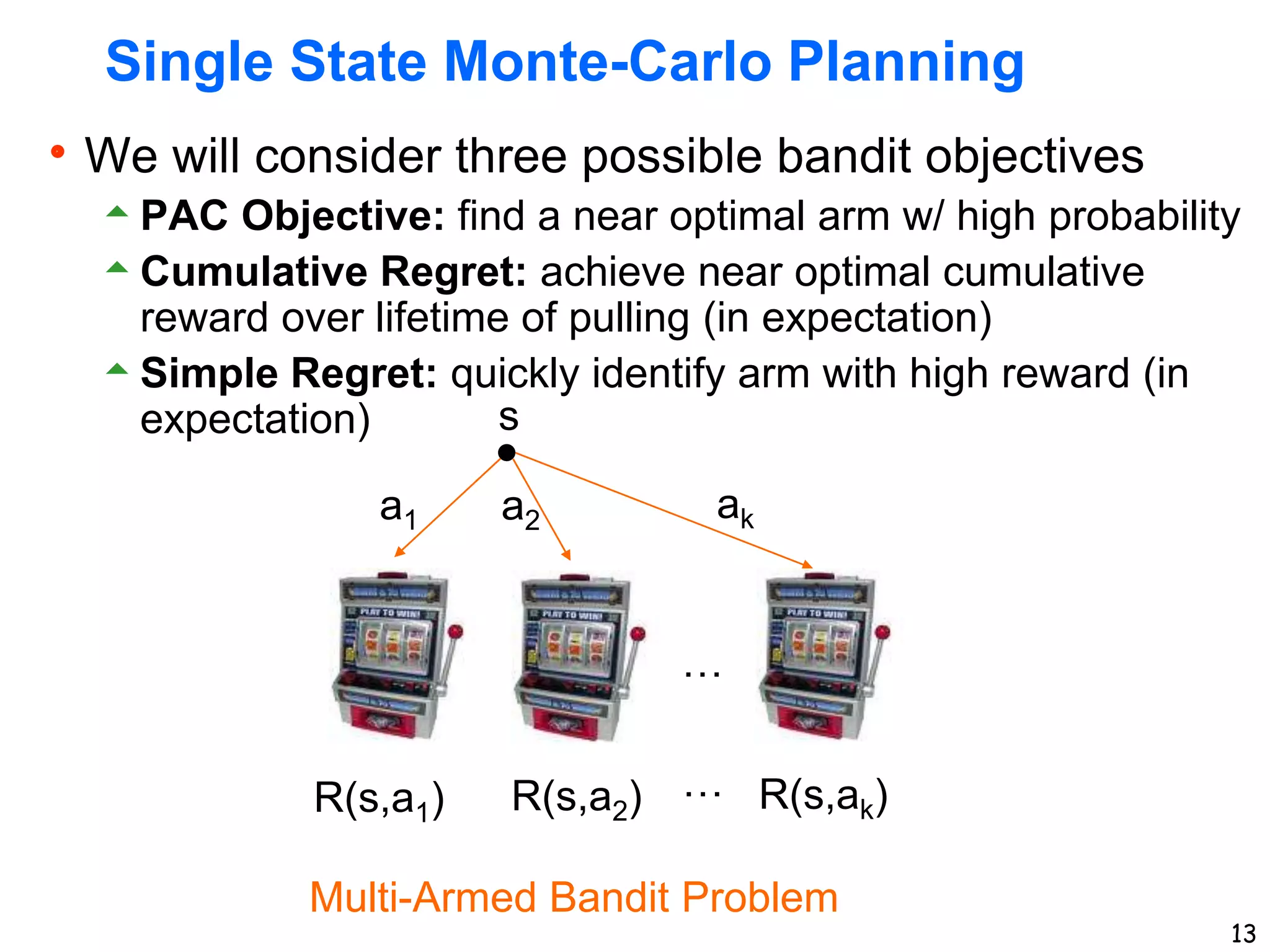
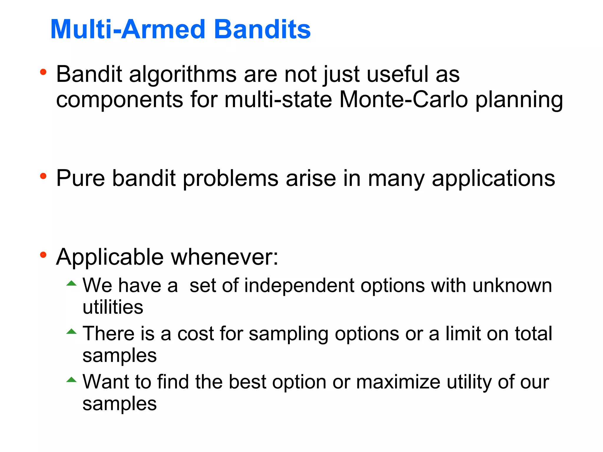
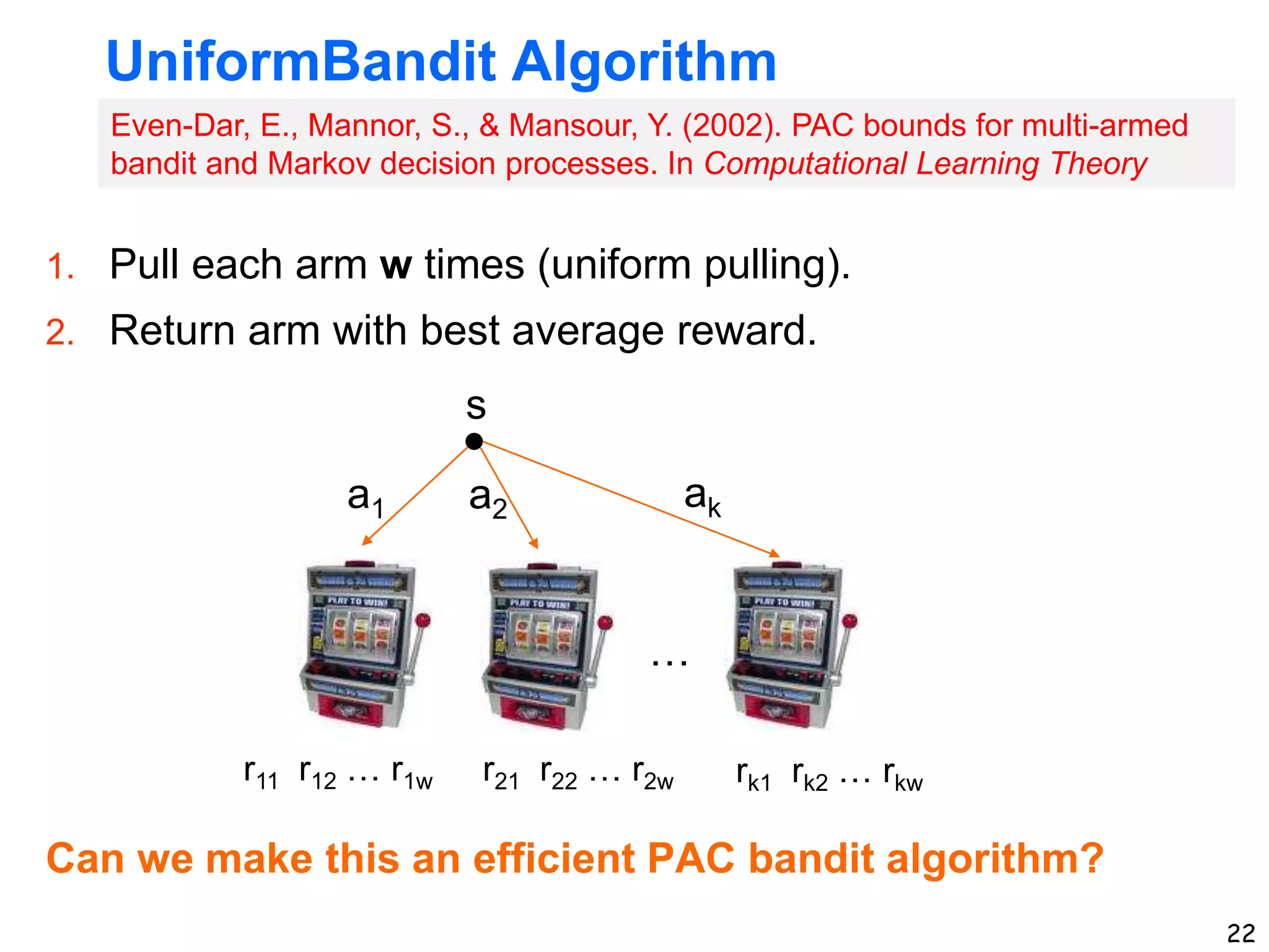
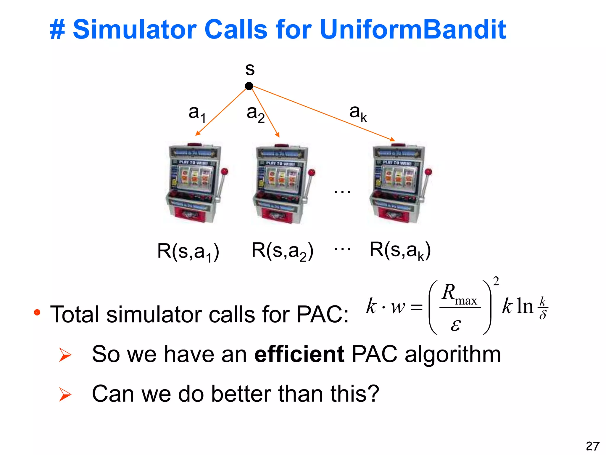
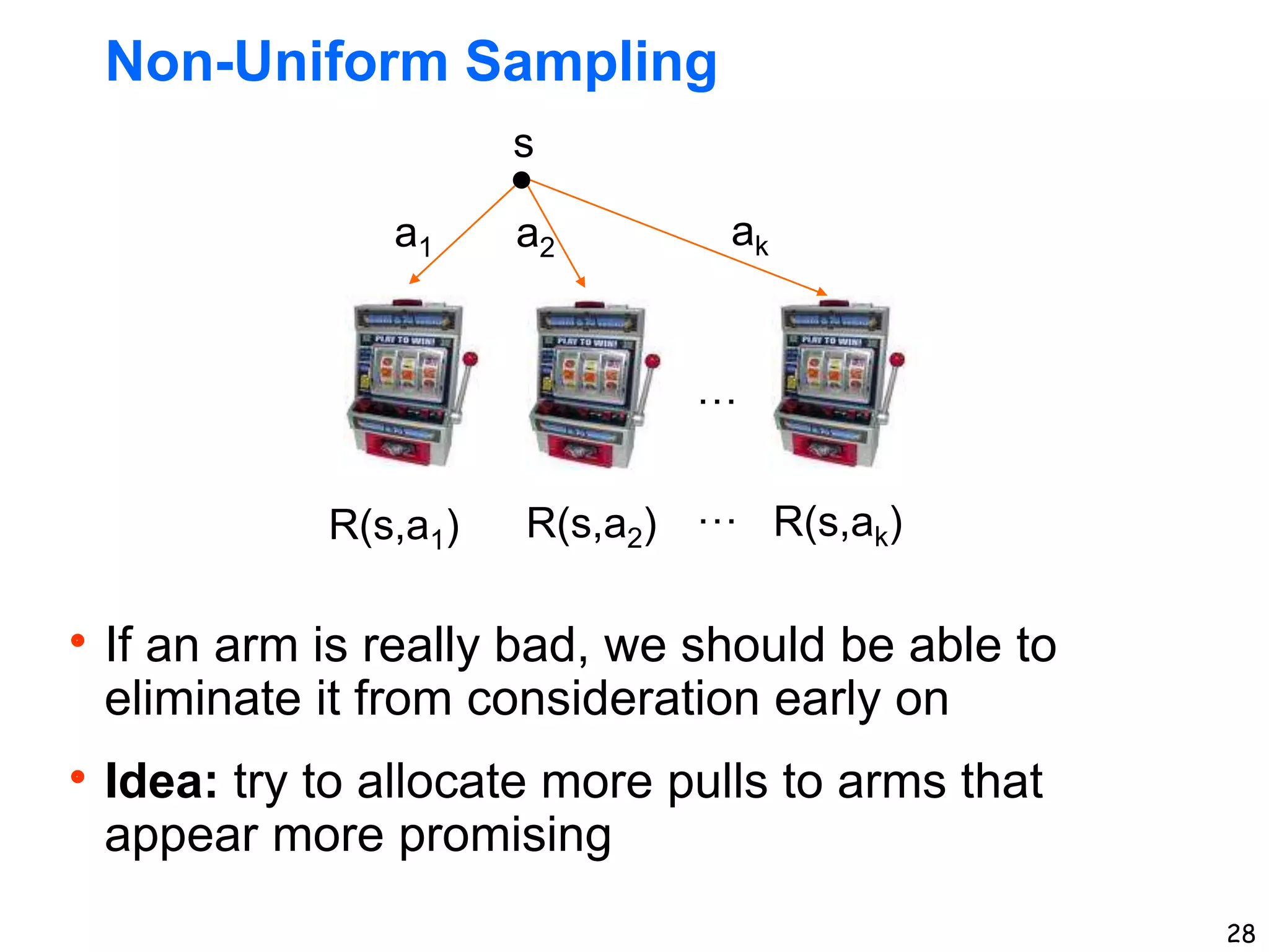
The document discusses approaches for planning in large worlds, including Monte-Carlo planning. It introduces the concept of a multi-armed bandit problem where an agent must choose between multiple actions with unknown rewards. The UniformBandit algorithm is analyzed, which pulls each arm a fixed number of times and selects the arm with the highest average reward. It is shown that by setting the number of pulls per arm appropriately, UniformBandit can be made into an efficient Probably Approximately Correct algorithm for the multi-armed bandit problem.

![Bounded Reward Assumption
A common assumption we will make is that
rewards are in a bounded interval [-𝑅𝑚𝑎𝑥, 𝑅𝑚𝑎𝑥].
I.e., for each 𝑖, Pr 𝑅 𝑠, 𝑎𝑖 ∈ −𝑅𝑚𝑎𝑥, 𝑅𝑚𝑎𝑥 = 1.
Results are available for other types of
assumptions, e.g. Gaussian distributions
Require different type of analysis](https://image.slidesharecdn.com/mcp-bandits-221119225015-ddfc7839/75/mcp-bandits-pptx-16-2048.jpg)

![20
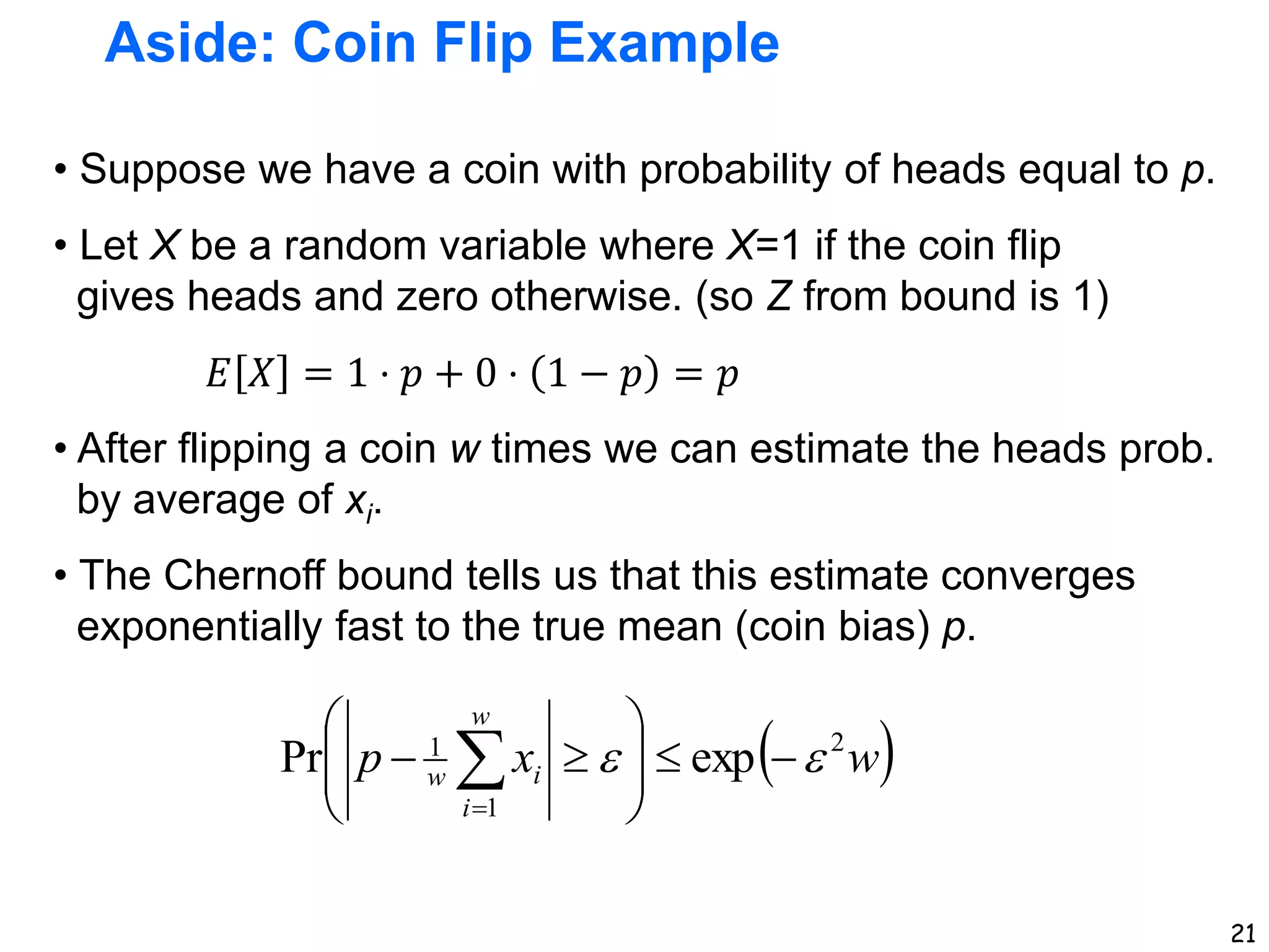
Aside: Additive Chernoff Bound
• Let R be a random variable with maximum absolute value Z.
An let ri i=1,…,w be i.i.d. samples of R
• The Chernoff bound gives a bound on the probability that the
average of the ri are far from E[R]
1
1
1
1
ln
]
[ w
w
i
i
w Z
r
R
E
With probability at least we have that,
1
w
Z
r
R
E
w
i
i
w
2
1
1
exp
]
[
Pr
Chernoff
Bound
Equivalent Statement:](https://image.slidesharecdn.com/mcp-bandits-221119225015-ddfc7839/75/mcp-bandits-pptx-20-2048.jpg)
![23
UniformBandit PAC Bound
• For a single bandit arm the Chernoff bound says (𝑍 = 𝑅𝑚𝑎𝑥):
• Bounding the error by ε gives:
• Thus, using this many samples for a single arm will guarantee
an ε-accurate estimate with probability at least
for a single arm.
'
1
1
max
1
1
ln
R
)]
,
(
[
w
w
j
ij
w
i r
a
s
R
E
With probability at least we have that,
'
1
'
1
1
max ln
w
R '
1
2
max
ln
R
w
or equivalently
'
1
](https://image.slidesharecdn.com/mcp-bandits-221119225015-ddfc7839/75/mcp-bandits-pptx-23-2048.jpg)

![26
UniformBandit PAC Bound
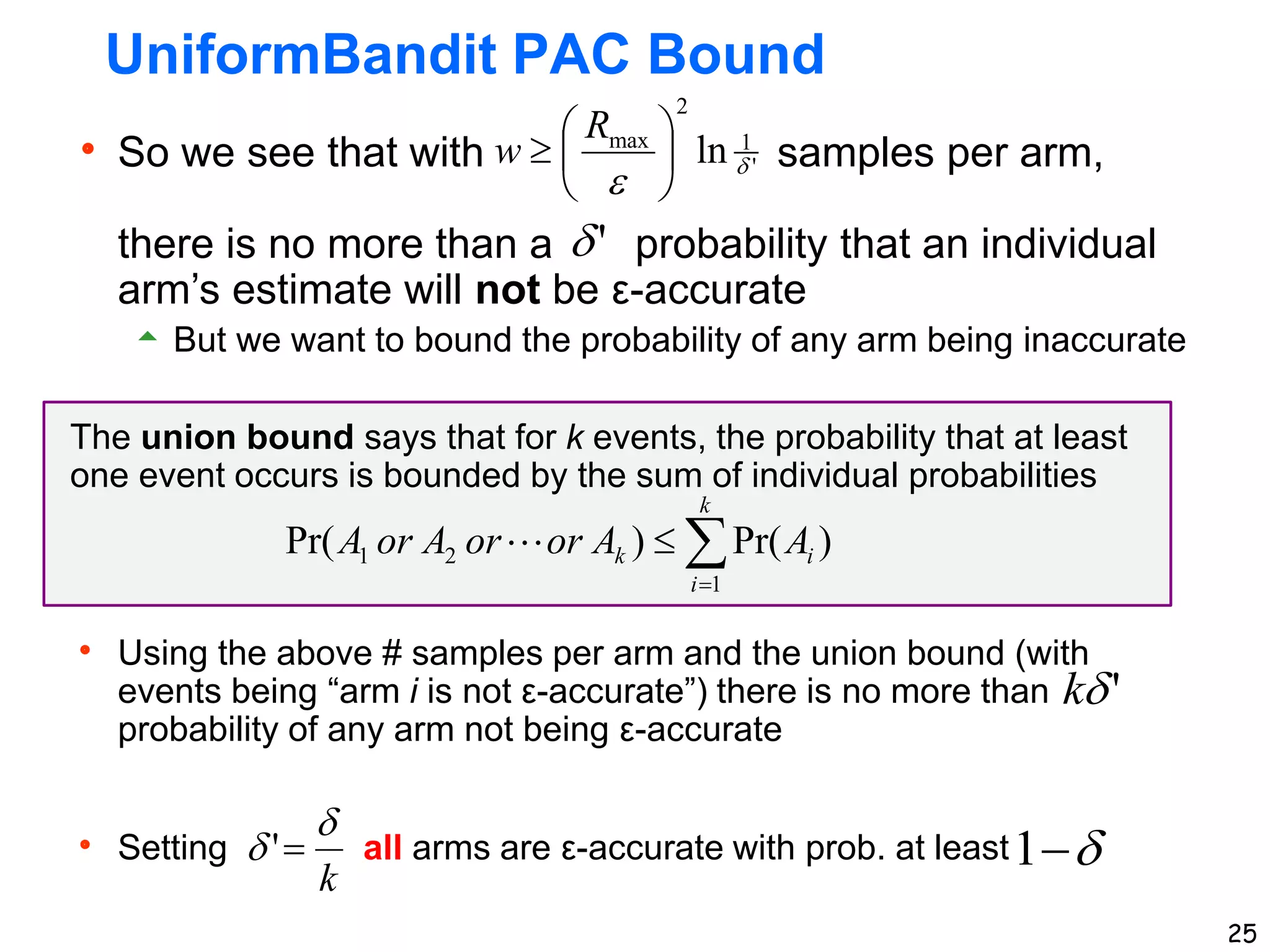
If then for all arms simultaneously
with probability at least
1
k
R
w ln
2
max
Putting everything together we get:
That is, estimates of all actions are ε – accurate
with probability at least 1-
Thus selecting estimate with highest value is
approximately optimal with high probability, or PAC
w
j
ij
w
i r
a
s
R
E
1
1
)]
,
(
[](https://image.slidesharecdn.com/mcp-bandits-221119225015-ddfc7839/75/mcp-bandits-pptx-26-2048.jpg)
![33
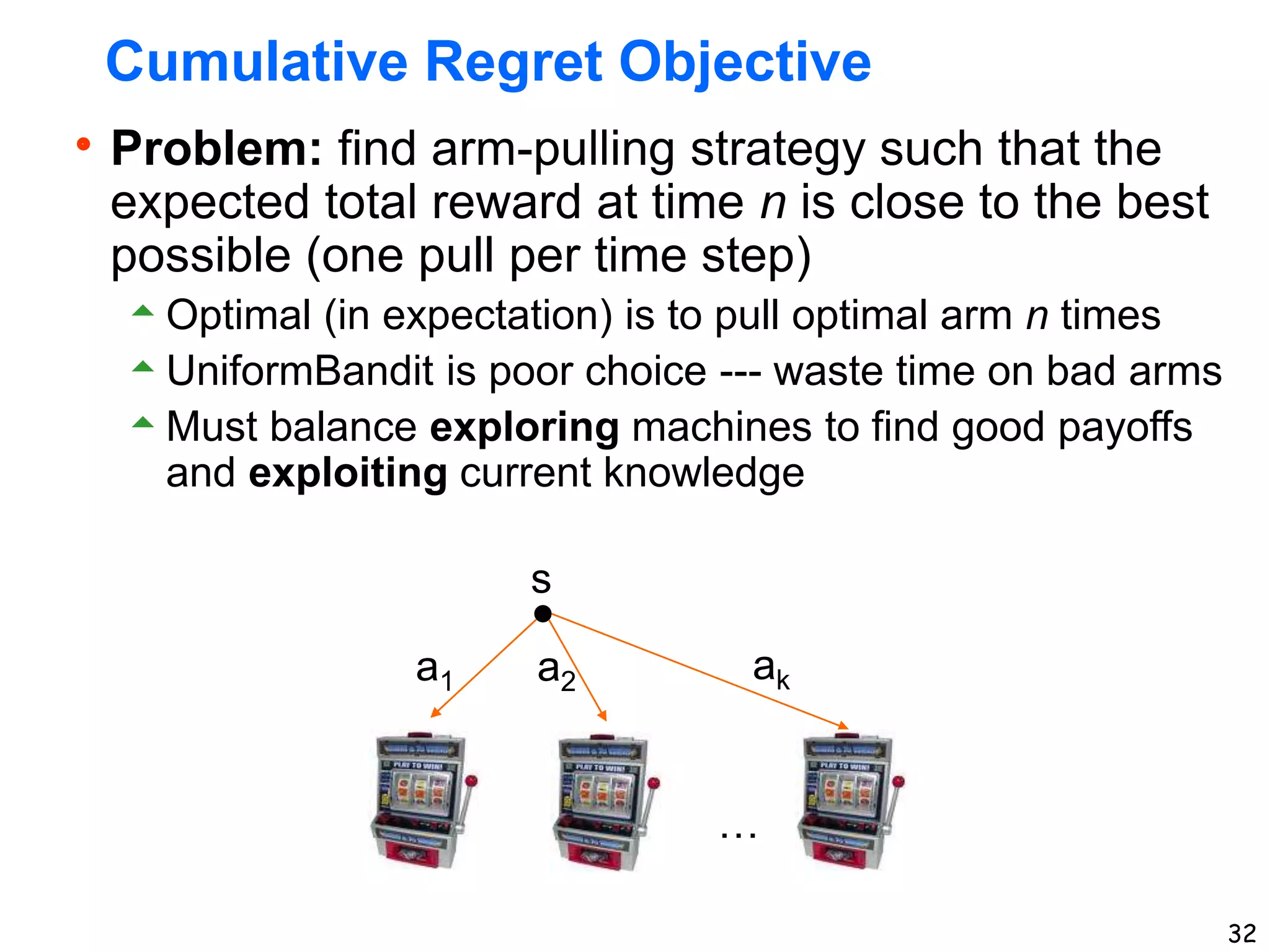
Cumulative Regret Objective
Theoretical results are often about “expected
cumulative regret” of an arm pulling strategy.
Protocol: At time step n the algorithm picks an
arm 𝑎𝑛 based on what it has seen so far and
receives reward 𝑟𝑛 (𝑎𝑛 and 𝑟𝑛 are random variables).
Expected Cumulative Regret (𝑬[𝑹𝒆𝒈𝒏]):
difference between optimal expected cummulative
reward and expected cumulative reward of our
strategy at time n
𝐸[𝑅𝑒𝑔𝑛] = 𝑛 ⋅ 𝑅∗ −
𝑖=1
𝑛
𝐸[𝑟𝑛]](https://image.slidesharecdn.com/mcp-bandits-221119225015-ddfc7839/75/mcp-bandits-pptx-33-2048.jpg)
![34
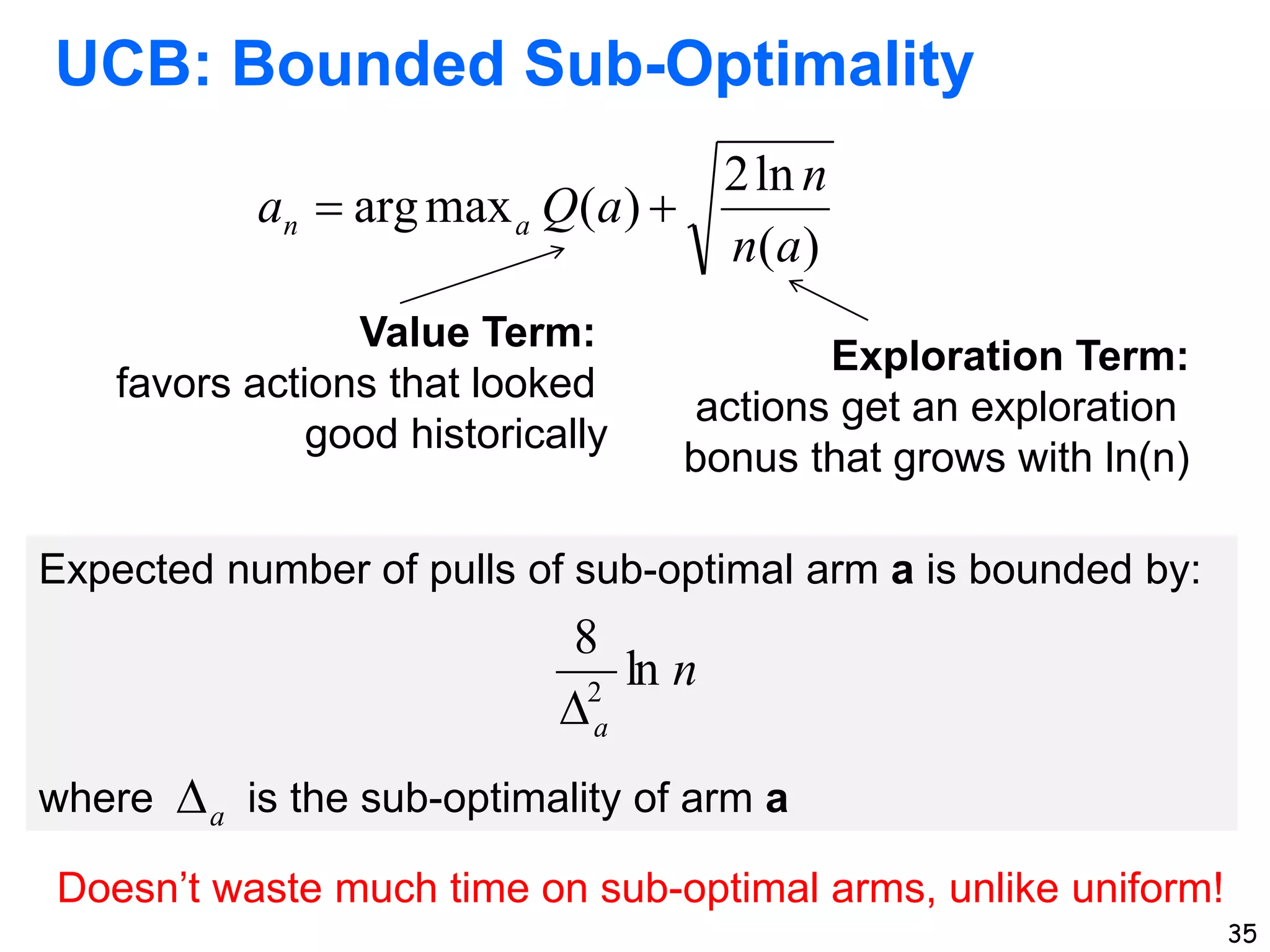
UCB Algorithm for Minimizing Cumulative Regret
Q(a) : average reward for trying action a (in
our single state s) so far
n(a) : number of pulls of arm a so far
Action choice by UCB after n pulls:
Assumes rewards in [0,1]. We can always
normalize given a bounded reward
assumption
)
(
ln
2
)
(
max
arg
a
n
n
a
Q
a a
n
Auer, P., Cesa-Bianchi, N., & Fischer, P. (2002). Finite-time analysis of the
multiarmed bandit problem. Machine learning, 47(2), 235-256.](https://image.slidesharecdn.com/mcp-bandits-221119225015-ddfc7839/75/mcp-bandits-pptx-34-2048.jpg)
![36
UCB Performance Guarantee
[Auer, Cesa-Bianchi, & Fischer, 2002]
Theorem: The expected cumulative regret of UCB
𝑬[𝑹𝒆𝒈𝒏] after n arm pulls is bounded by O(log n)
Is this good?
Yes. The average per-step regret is O
log 𝑛
𝑛
Theorem: No algorithm can achieve a better
expected regret (up to constant factors)](https://image.slidesharecdn.com/mcp-bandits-221119225015-ddfc7839/75/mcp-bandits-pptx-36-2048.jpg)
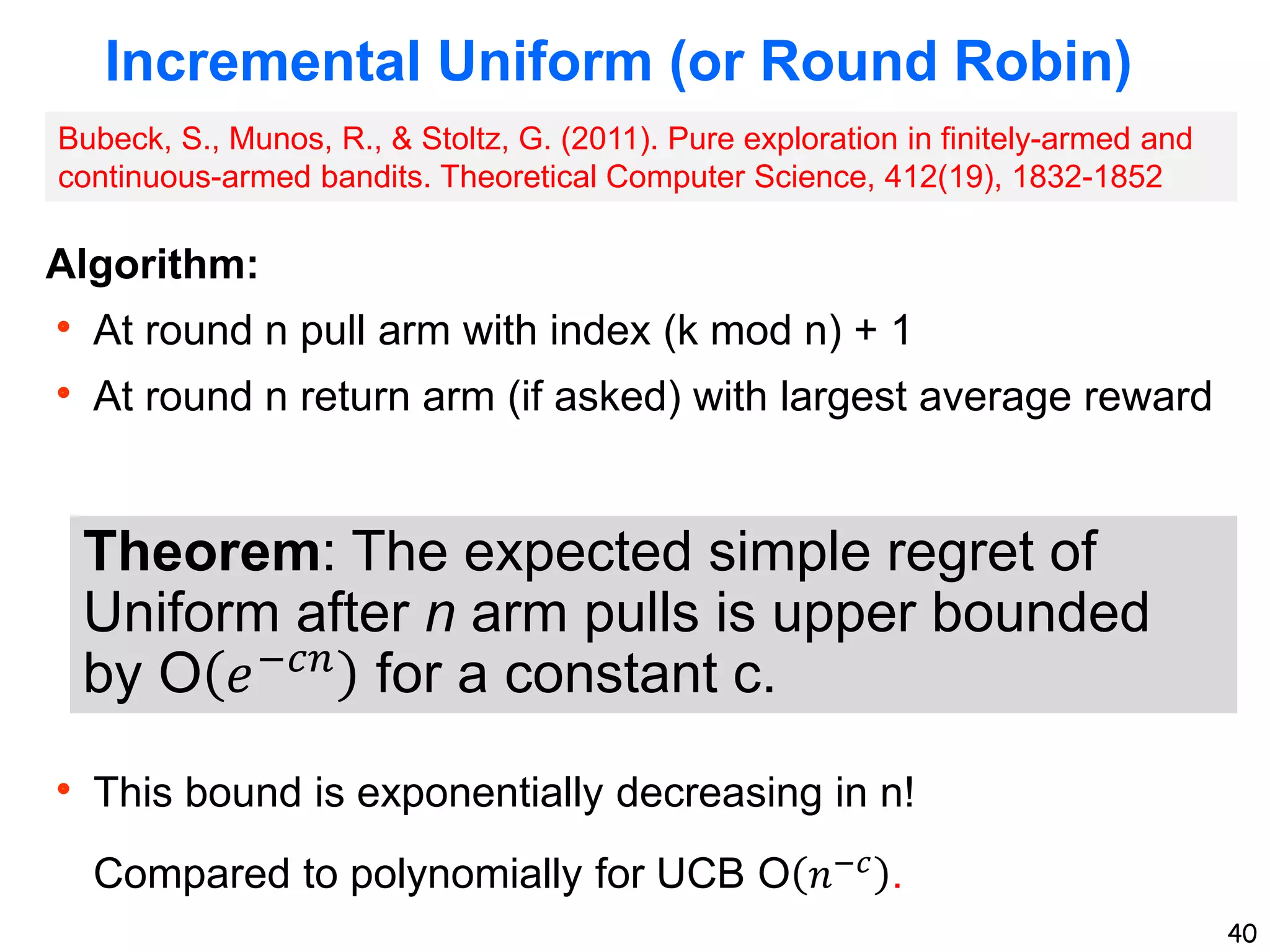
![38
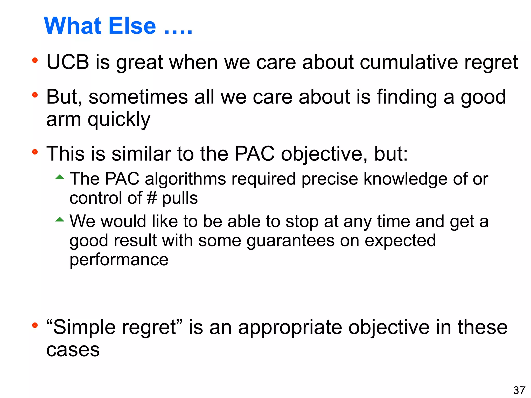
Simple Regret Objective
Protocol: At time step n the algorithm picks an
“exploration” arm 𝑎𝑛 to pull and observes reward
𝑟𝑛 and also picks an arm index it thinks is best 𝑗𝑛
(𝑎𝑛, 𝑗𝑛 and 𝑟𝑛 are random variables).
If interrupted at time n the algorithm returns 𝑗𝑛.
Expected Simple Regret (𝑬[𝑺𝑹𝒆𝒈𝒏]): difference
between 𝑅∗
and expected reward of arm 𝑗𝑛
selected by our strategy at time n
𝐸[𝑆𝑅𝑒𝑔𝑛] = 𝑅∗ − 𝐸[𝑅(𝑎𝑗𝑛
)]](https://image.slidesharecdn.com/mcp-bandits-221119225015-ddfc7839/75/mcp-bandits-pptx-38-2048.jpg)


![[DSC Europe 25] Marko Krstic - Understanding the AI Threat Landscape - Risks,...](https://cdn.slidesharecdn.com/ss_thumbnails/tiyim1ins5jvbrvzpzla-2-251209104645-c69d3553-thumbnail.jpg?width=640&height=640&fit=bounds)
![[DSC Europe 25] Jovan Bogicevic - Legacy to AI-Driven Defense: Transforming D...](https://cdn.slidesharecdn.com/ss_thumbnails/rsarluadt563hntyfc8q-3-251211083849-3e7bc4c0-thumbnail.jpg?width=640&height=640&fit=bounds)

![[DSC Europe 25] Branko Urosevic -Rethinking Financial Talent: Integrating Cod...](https://cdn.slidesharecdn.com/ss_thumbnails/8jjrus8ttko6qj64f58f-3-251212103250-642c6374-thumbnail.jpg?width=640&height=640&fit=bounds)
![[DSC Europe 25] Nikolay Burlutskiy - Best Practices for Building Enterprise M...](https://cdn.slidesharecdn.com/ss_thumbnails/uirvaiuvq8y1w8hzd9tx-7-251212103249-2619edb4-thumbnail.jpg?width=640&height=640&fit=bounds)


![[DSC Europe 25] Dragana Ilic - AI for Big Data in Astronomy.pptx](https://cdn.slidesharecdn.com/ss_thumbnails/8palya86qaatvjhva1ms-2-dragana-ilic-ai-ilic-251208151906-652b819c-thumbnail.jpg?width=640&height=640&fit=bounds)

![[DSC Europe 25] Sara Polak - The Archaeology of Innovation: AI as the Next Cr...](https://cdn.slidesharecdn.com/ss_thumbnails/7ecbscdnt8mlcuqbd2ln-2-sara-polak-ai-creative-industries-251208152533-aa1fcf54-thumbnail.jpg?width=640&height=640&fit=bounds)

![[DSC Europe 25] Aleksandra Dragicevic - AI-Boosted Research in Healthcare: Fr...](https://cdn.slidesharecdn.com/ss_thumbnails/iqwngszurf2r7pi1lnnj-4-aleksandra-dragicevic-ad-dsc-europe-conference-20-251208151905-37c3238a-thumbnail.jpg?width=640&height=640&fit=bounds)