DISCLAIMER
This work wasproduced by Dr. Adria Junyent-Ferre and Dr. Joan Marc Rodriguez-Bernuz
under the Global Power System Transformation Consortium. This work is not for commercial
purposes. The views expressed in this material do not necessarily represent the views of the
Department of Energy or the U.S. Government, or any agency thereof, including Imperial
College London or Imperial Consultants.
3.
Learn more aboutthe Global Power System Transformation (G-PST)
Consortium and the team from Imperial College London.
• Visit the G-PST website.
• Learn more about the G-PST’s Foundational Workforce Development Pillar.
|
Connect with the G-PST on
social media to stay up to date
on Women in PST, research,
free trainings, and curriculum.
4.
Global Power SystemTransformation Consortium | 4
Contents Summary
• Context
• Scaling voltage source converter (VSC) topologies to HVDC voltage levels
• How does 2-lvl VSC topologies scale to HVDC?
• Converter topologies: Series Insulated Gate Bipolar Transistors (IGBT), Half-Bridge, Full-Bridge.
• Comparison of pros & cons of VSC-HVDC topologies.
• Basics of MMC (a simplified single-phase case)
• Principles of MMC operation:
• Derivation of an equivalent average model.
• Steady-state equations analysis:
• Understanding system components: sum. and diff. transformations.
• Understanding energy exchange within the arm.
• Summary of steady-state equations.
• Exercise 1: Derive converter limits based on the steady-state analysis.
Global Power SystemTransformation Consortium | 6
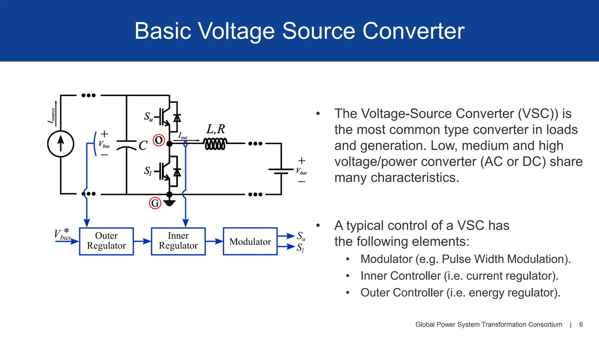
Basic Voltage Source Converter
• The Voltage-Source Converter (VSC)) is
the most common type converter in loads
and generation. Low, medium and high
voltage/power converter (AC or DC) share
many characteristics.
• A typical control of a VSC has
the following elements:
• Modulator (e.g. Pulse Width Modulation).
• Inner Controller (i.e. current regulator).
• Outer Controller (i.e. energy regulator).
7.
Global Power SystemTransformation Consortium | 7
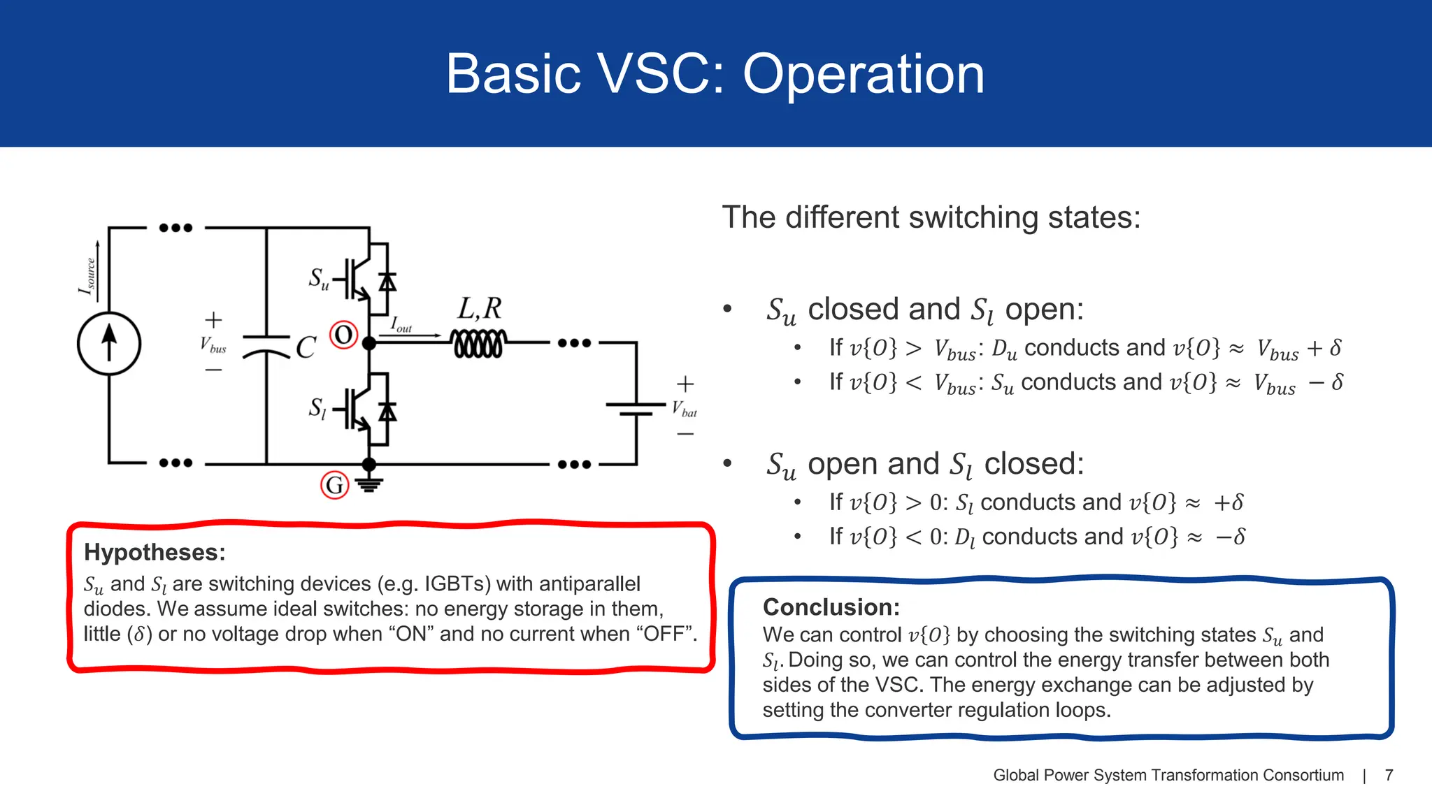
Basic VSC: Operation
The different switching states:
• 𝑆𝑢 closed and 𝑆𝑙 open:
• If 𝑣 𝑂 > 𝑉𝑏𝑢𝑠: 𝐷𝑢 conducts and 𝑣 𝑂 ≈ 𝑉𝑏𝑢𝑠 + 𝛿
• If 𝑣 𝑂 < 𝑉𝑏𝑢𝑠: 𝑆𝑢 conducts and 𝑣 𝑂 ≈ 𝑉𝑏𝑢𝑠 − 𝛿
• 𝑆𝑢 open and 𝑆𝑙 closed:
• If 𝑣 𝑂 > 0: 𝑆𝑙 conducts and 𝑣 𝑂 ≈ +𝛿
• If 𝑣 𝑂 < 0: 𝐷𝑙 conducts and 𝑣 𝑂 ≈ −𝛿
Conclusion:
We can control 𝑣 𝑂 by choosing the switching states 𝑆𝑢 and
𝑆𝑙. Doing so, we can control the energy transfer between both
sides of the VSC. The energy exchange can be adjusted by
setting the converter regulation loops.
Hypotheses:
𝑆𝑢 and 𝑆𝑙 are switching devices (e.g. IGBTs) with antiparallel
diodes. We assume ideal switches: no energy storage in them,
little (𝛿) or no voltage drop when “ON” and no current when “OFF”.
8.
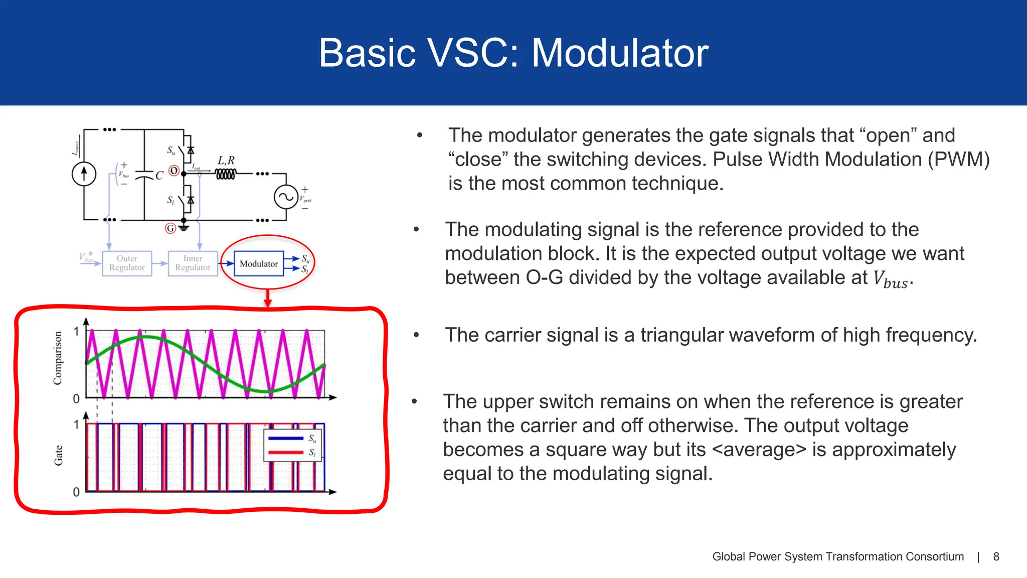
Global Power SystemTransformation Consortium | 8
Basic VSC: Modulator
• The modulator generates the gate signals that “open” and
“close” the switching devices. Pulse Width Modulation (PWM)
is the most common technique.
• The modulating signal is the reference provided to the
modulation block. It is the expected output voltage we want
between O-G divided by the voltage available at 𝑉𝑏𝑢𝑠.
• The carrier signal is a triangular waveform of high frequency.
• The upper switch remains on when the reference is greater
than the carrier and off otherwise. The output voltage
becomes a square way but its <average> is approximately
equal to the modulating signal.
9.
Global Power SystemTransformation Consortium | 9
Basic VSC: Inner Regulator
• The inner regulator is the block that generates reference signals
for the modulator. This block normally regulates the converter
output’s current to guarantee this magnitude is within the
physical limits of the hardware.
𝐿
𝑑
𝑑𝑡
+ 𝑅 𝑖𝑜𝑢𝑡 𝑡 = 𝑣𝑂 𝑡 − 𝑣𝑔𝑟𝑖𝑑(𝑡)
𝐼𝑜𝑢𝑡 =
1
𝑠𝐿 + 𝑅
𝑉𝑂 −
1
𝑠𝐿 + 𝑅
𝑉𝑔𝑟𝑖𝑑
Control plant disturbance plant
• The dynamic link between the output current
and the voltage applied by the modulator is
dictated by the output filter:
• When designing the controller, we use this
equation expressed in Laplace variables:
𝐺(𝑠) =
𝐼𝑜𝑢𝑡(𝑠)
𝑉𝑂(𝑠)
=
1
𝑅
𝐿
𝑅
𝑠 + 1
=
𝐴
1
𝜏
𝑠 + 1
• The open loop transfer
function is of the form
• The closed-loop control diagram looks as follows:
10.
Global Power SystemTransformation Consortium | 10
Basic VSC: Inner Regulator
[1] Sigurd Skogestad and Ian Postlethwaite. 2005. Multivariable Feedback Control:
Analysis and Design. John Wiley & Sons, Inc., Hoboken, NJ, USA.
• Different techniques can be used to design the
inner regulator (e.g. PI, PR, ℋ∞,etc.). For instance,
a PI can be used to track a DC reference, which
can be easily tuned following the Internal Model
Control (IMC) technique. The inner regulator can
be tuned based on the plant and desired system
time-constant 𝜏. [1]
If we use a PI as a regulator: 𝐾 𝑠 = 𝐾𝑝 +
𝐾𝐼
𝑠
The closed-loop function becomes: 𝑇 𝑠 =
𝐼𝑜𝑢𝑡(𝑠)
𝐼𝑜𝑢𝑡
∗
(𝑠)
=
𝐺 𝑠 𝐾(𝑠)
1 + 𝐺 𝑠 𝐾(𝑠)
≈
1
𝜏𝑠 + 1
with the following PI gains... 𝐾𝑝 =
𝐿
𝜏
and 𝐾𝐼 =
𝑅
𝜏
Simulation example: 𝐿 = 100 uH, 𝑅= 1 𝑚Ω, 𝑉𝑏𝑎𝑡 = 50 V, 𝑉𝑏𝑢𝑠 = 100 V. 𝜏 = 10 ms.
𝐾𝑝 = 0.01 and 𝐾𝐼 = 0.1. The input reference 𝐼𝑜𝑢𝑡
∗
does a step change from 0 to 10 at
time 0.1 s. (see file: inner_regulator_example.mo)
Closed-loop time
response show 63% of
final value is achieved
10 ms after change.
11.
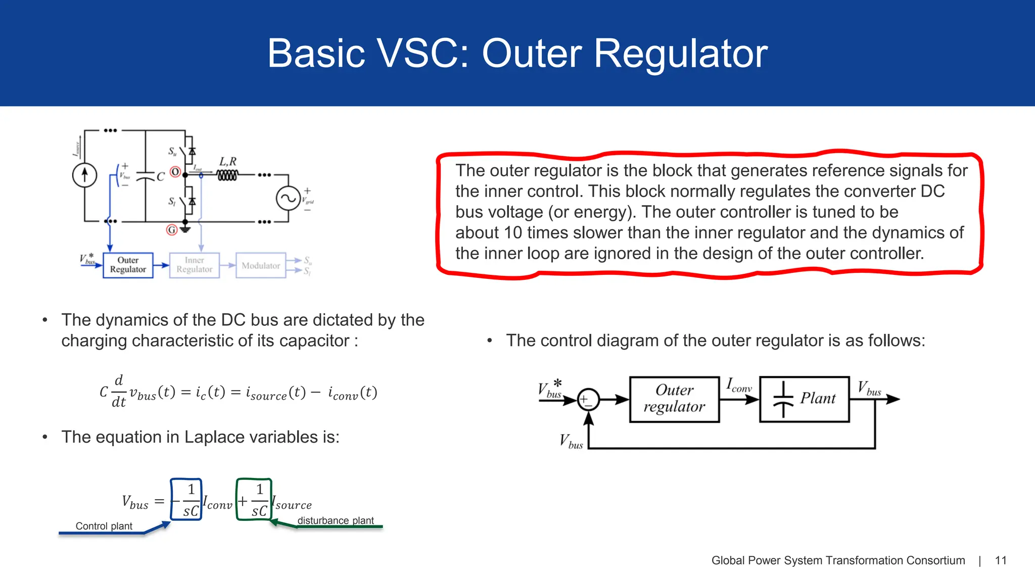
Global Power SystemTransformation Consortium | 11
Basic VSC: Outer Regulator
The outer regulator is the block that generates reference signals for
the inner control. This block normally regulates the converter DC
bus voltage (or energy). The outer controller is tuned to be
about 10 times slower than the inner regulator and the dynamics of
the inner loop are ignored in the design of the outer controller.
• The dynamics of the DC bus are dictated by the
charging characteristic of its capacitor :
• The equation in Laplace variables is:
• The control diagram of the outer regulator is as follows:
𝐶
𝑑
𝑑𝑡
𝑣𝑏𝑢𝑠 𝑡 = 𝑖𝑐 𝑡 = 𝑖𝑠𝑜𝑢𝑟𝑐𝑒(𝑡) − 𝑖𝑐𝑜𝑛𝑣(𝑡)
Control plant
disturbance plant
𝑉𝑏𝑢𝑠 = −
1
𝑠𝐶
𝐼𝑐𝑜𝑛𝑣 +
1
𝑠𝐶
𝐼𝑠𝑜𝑢𝑟𝑐𝑒
12.
Global Power SystemTransformation Consortium | 12
Basic VSC: Outer Regulator
The gains are set to give a specific maximum transient error
of Δ𝑉𝑏𝑢𝑠
𝑀𝐴𝑋
for a sudden change of the current fed to the DC
bus of Δ𝐼𝑠𝑜𝑢𝑟𝑐𝑒
𝑀𝐴𝑋
.
[1] Sigurd Skogestad and Ian Postlethwaite. 2005. Multivariable Feedback Control:
Analysis and Design. John Wiley & Sons, Inc., Hoboken, NJ, USA.
Gains for specified peak transient error:
𝐾𝑃 = −
𝟐𝚫𝑰𝑠𝑜𝑢𝑟𝑐𝑒
𝑴𝑨𝑿
𝒆𝚫𝑽𝑏𝑢𝑠
𝑴𝑨𝑿
𝐾𝐼 = −
𝑲𝑷
𝟐
𝟒𝑪
Figure: Outer regulator response to a step-change of the current
fed to the DC bus and to a change of Vbus reference.
Δ𝑉𝑏𝑢𝑠
𝑀𝐴𝑋
Global Power SystemTransformation Consortium | 14
Context
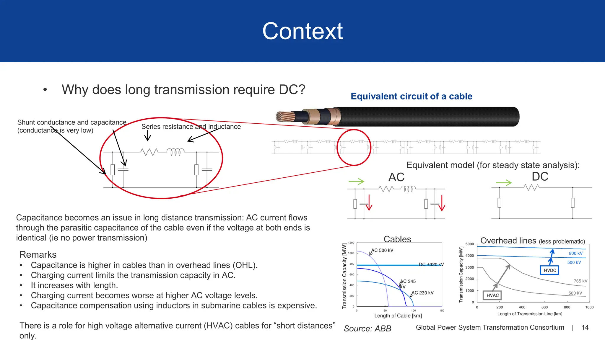
• Why does long transmission require DC? Equivalent circuit of a cable
Series resistance and inductance
Shunt conductance and capacitance
(conductance is very low)
Equivalent model (for steady state analysis):
AC DC
Cables Overhead lines (less problematic)
Remarks
• Capacitance is higher in cables than in overhead lines (OHL).
• Charging current limits the transmission capacity in AC.
• It increases with length.
• Charging current becomes worse at higher AC voltage levels.
• Capacitance compensation using inductors in submarine cables is expensive.
There is a role for high voltage alternative current (HVAC) cables for “short distances”
only.
Capacitance becomes an issue in long distance transmission: AC current flows
through the parasitic capacitance of the cable even if the voltage at both ends is
identical (ie no power transmission)
Source: ABB
15.
Global Power SystemTransformation Consortium | 15
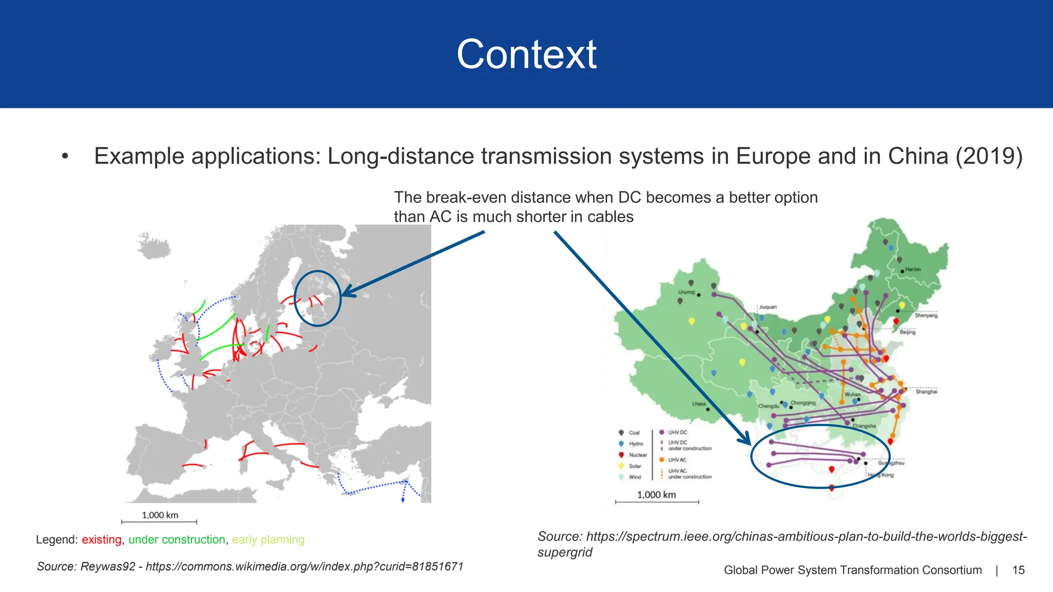
Context
• Example applications: Long-distance transmission systems in Europe and in China (2019)
The break-even distance when DC becomes a better option
than AC is much shorter in cables
Source: https://spectrum.ieee.org/chinas-ambitious-plan-to-build-the-worlds-biggest-
supergrid
Legend: existing, under construction, early planning
Source: Reywas92 - https://commons.wikimedia.org/w/index.php?curid=81851671
16.
Global Power SystemTransformation Consortium | 16
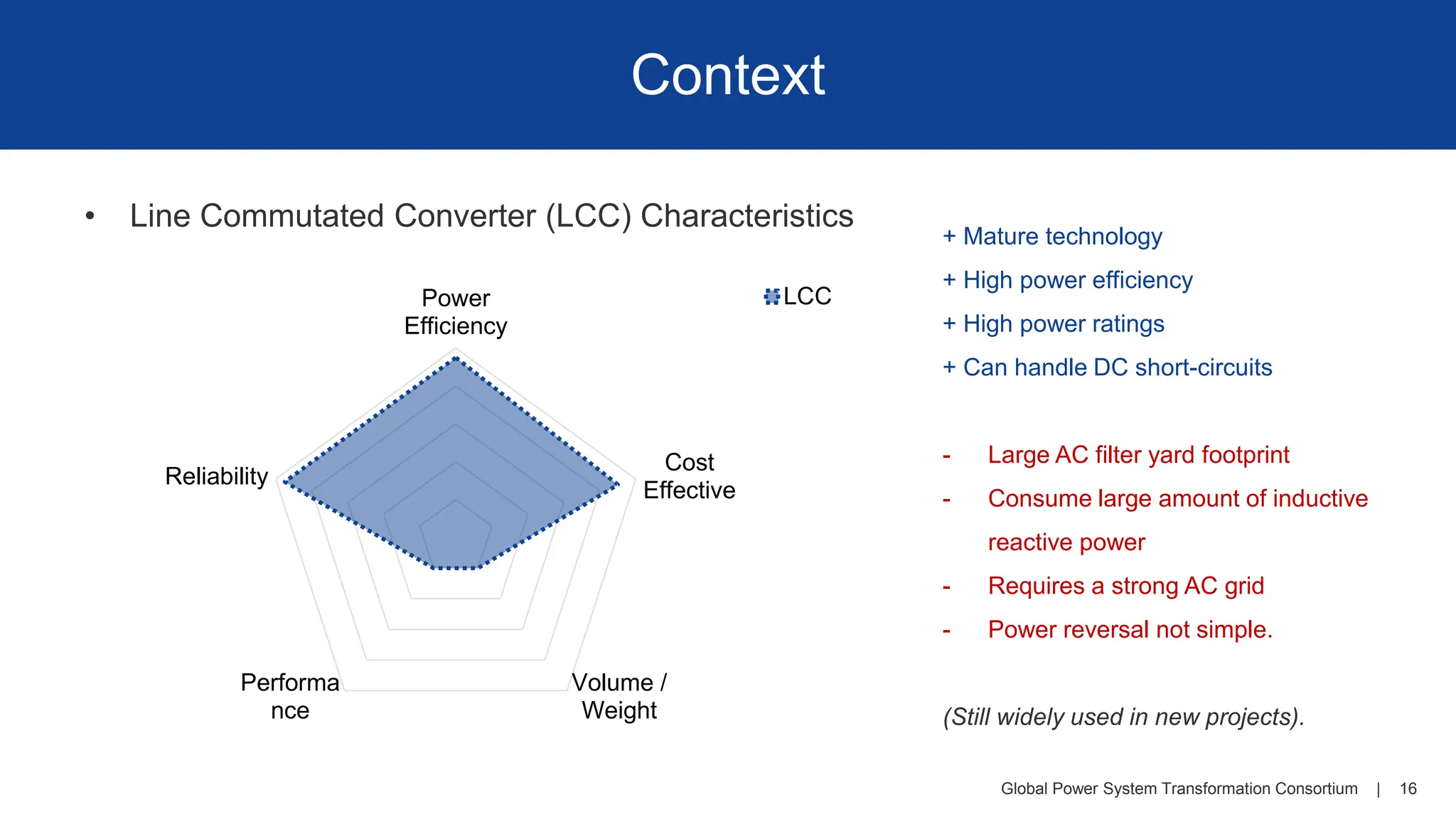
Context
• Line Commutated Converter (LCC) Characteristics
Power
Efficiency
Cost
Effective
Volume /
Weight
Performa
nce
Reliability
LCC
+ Mature technology
+ High power efficiency
+ High power ratings
+ Can handle DC short-circuits
- Large AC filter yard footprint
- Consume large amount of inductive
reactive power
- Requires a strong AC grid
- Power reversal not simple.
(Still widely used in new projects).
17.
Global Power SystemTransformation Consortium | 17
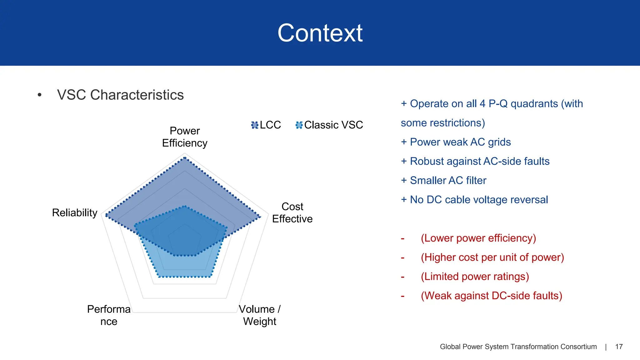
Context
• VSC Characteristics
+ Operate on all 4 P-Q quadrants (with
some restrictions)
+ Power weak AC grids
+ Robust against AC-side faults
+ Smaller AC filter
+ No DC cable voltage reversal
- (Lower power efficiency)
- (Higher cost per unit of power)
- (Limited power ratings)
- (Weak against DC-side faults)
Power
Efficiency
Cost
Effective
Volume /
Weight
Performa
nce
Reliability
LCC Classic VSC
18.
Global Power SystemTransformation Consortium | 18
Context
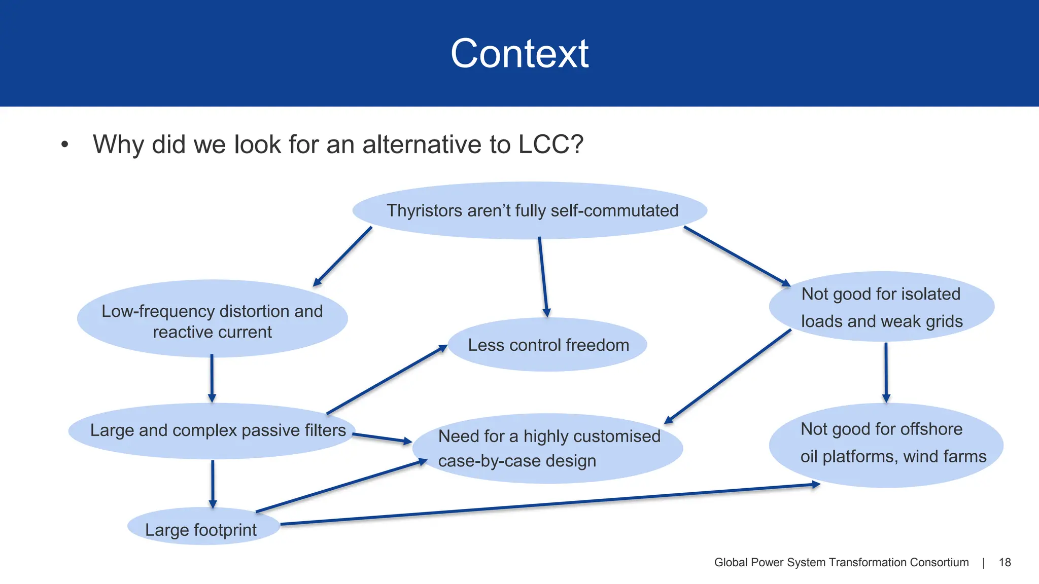
• Why did we look for an alternative to LCC?
Thyristors aren’t fully self-commutated
Low-frequency distortion and
reactive current
Large and complex passive filters
Large footprint
Less control freedom
Need for a highly customised
case-by-case design
Not good for isolated
loads and weak grids
Not good for offshore
oil platforms, wind farms
19.
Global Power SystemTransformation Consortium | 19
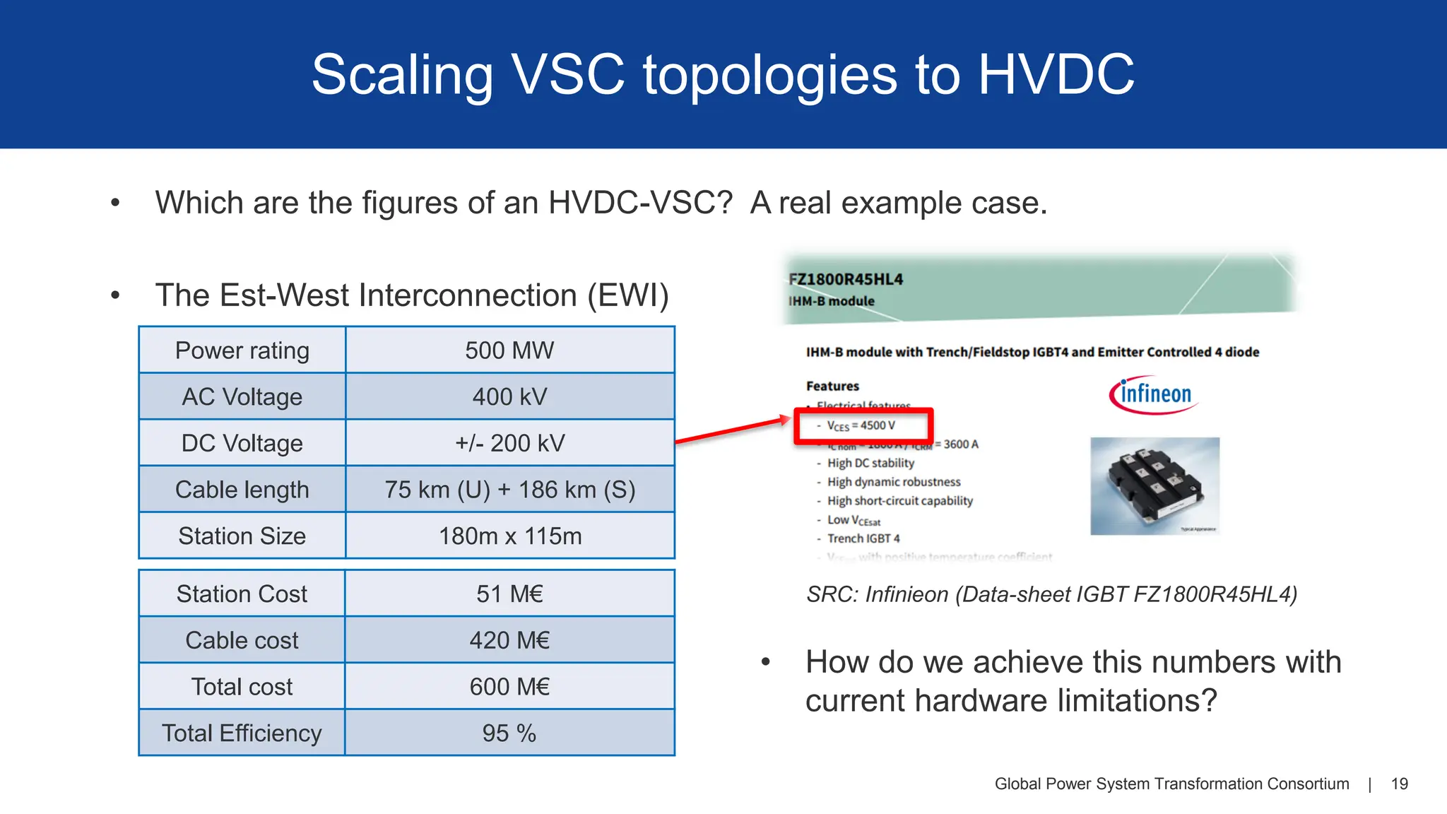
Scaling VSC topologies to HVDC
• Which are the figures of an HVDC-VSC? A real example case.
• The Est-West Interconnection (EWI)
w
Power rating 500 MW
AC Voltage 400 kV
DC Voltage +/- 200 kV
Cable length 75 km (U) + 186 km (S)
Station Size 180m x 115m
Station Cost 51 M€
Cable cost 420 M€
Total cost 600 M€
Total Efficiency 95 %
• How do we achieve this numbers with
current hardware limitations?
SRC: Infinieon (Data-sheet IGBT FZ1800R45HL4)
20.
Global Power SystemTransformation Consortium | 20
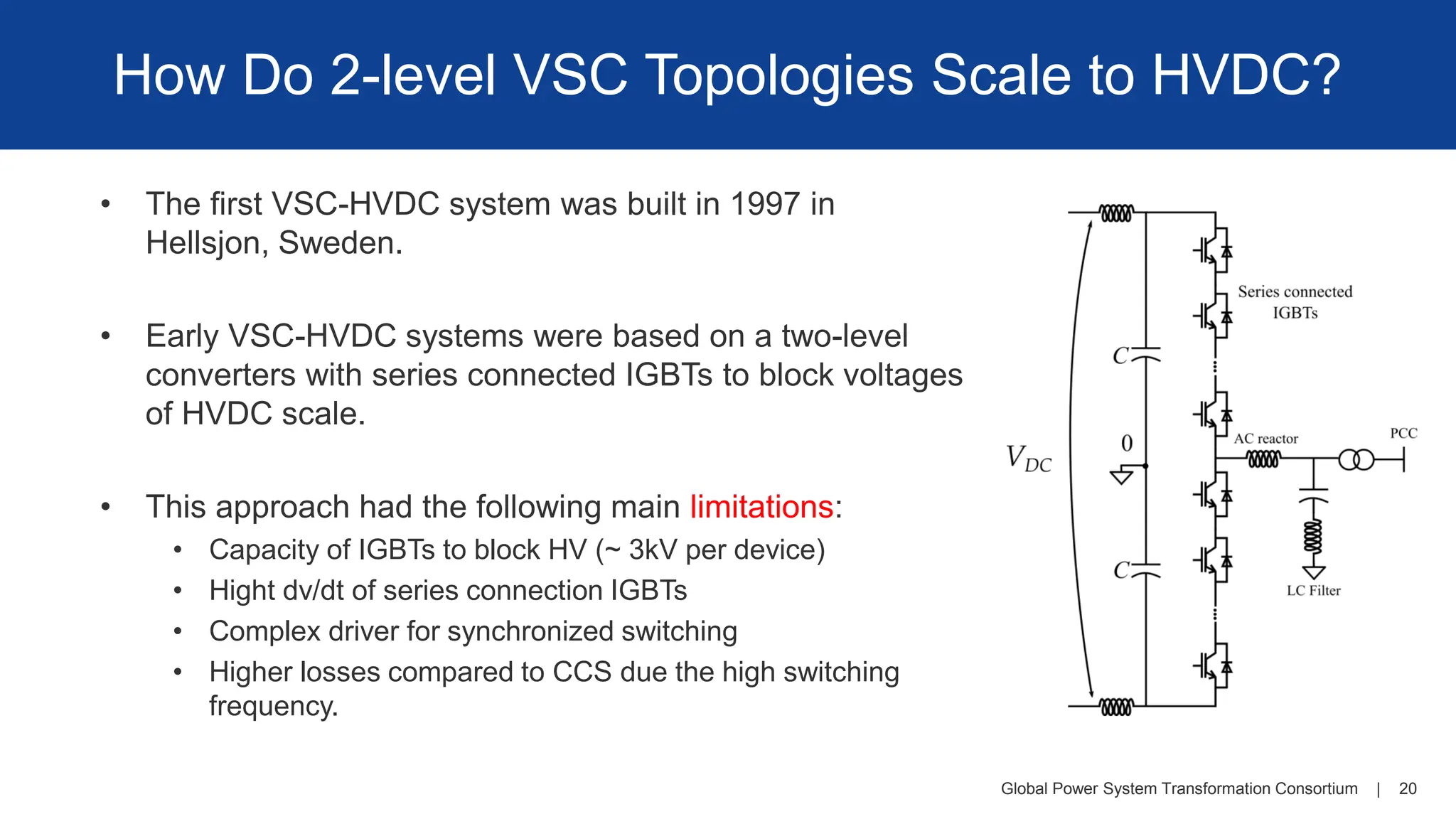
How Do 2-level VSC Topologies Scale to HVDC?
• The first VSC-HVDC system was built in 1997 in
Hellsjon, Sweden.
• Early VSC-HVDC systems were based on a two-level
converters with series connected IGBTs to block voltages
of HVDC scale.
• This approach had the following main limitations:
• Capacity of IGBTs to block HV (~ 3kV per device)
• Hight dv/dt of series connection IGBTs
• Complex driver for synchronized switching
• Higher losses compared to CCS due the high switching
frequency.
21.
Global Power SystemTransformation Consortium | 22
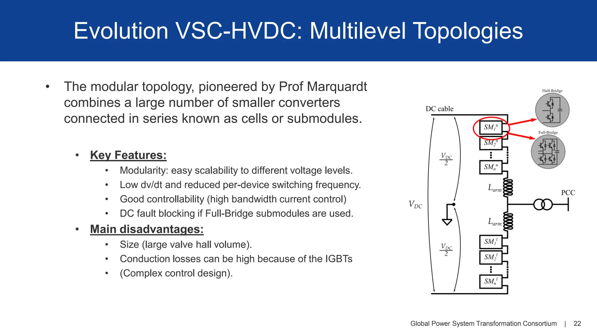
Evolution VSC-HVDC: Multilevel Topologies
• The modular topology, pioneered by Prof Marquardt
combines a large number of smaller converters
connected in series known as cells or submodules.
• Key Features:
• Modularity: easy scalability to different voltage levels.
• Low dv/dt and reduced per-device switching frequency.
• Good controllability (high bandwidth current control)
• DC fault blocking if Full-Bridge submodules are used.
• Main disadvantages:
• Size (large valve hall volume).
• Conduction losses can be high because of the IGBTs
• (Complex control design).
22.
Global Power SystemTransformation Consortium | 23
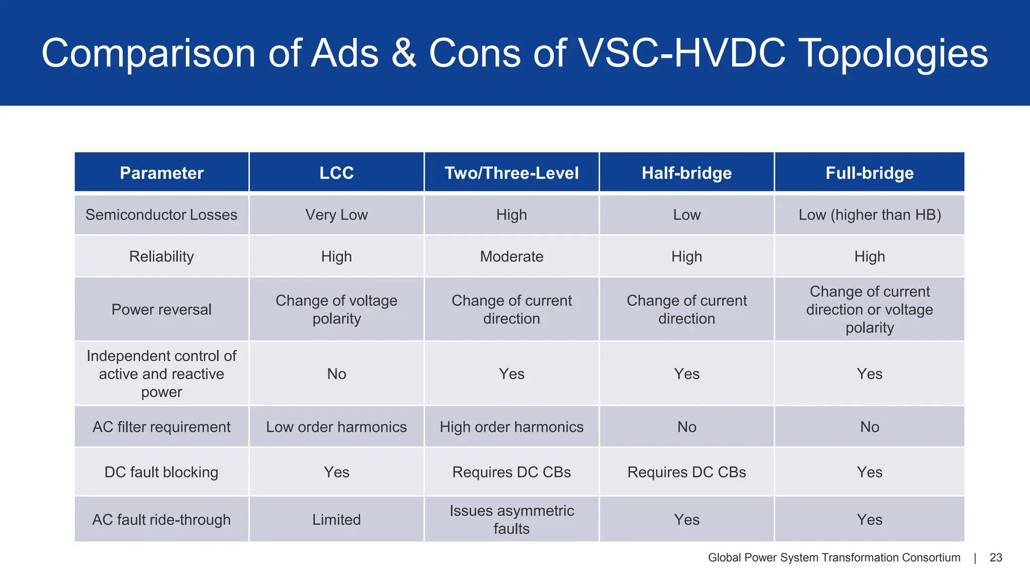
Comparison of Ads & Cons of VSC-HVDC Topologies
Parameter LCC Two/Three-Level Half-bridge Full-bridge
Semiconductor Losses Very Low High Low Low (higher than HB)
Reliability High Moderate High High
Power reversal
Change of voltage
polarity
Change of current
direction
Change of current
direction
Change of current
direction or voltage
polarity
Independent control of
active and reactive
power
No Yes Yes Yes
AC filter requirement Low order harmonics High order harmonics No No
DC fault blocking Yes Requires DC CBs Requires DC CBs Yes
AC fault ride-through Limited
Issues asymmetric
faults
Yes Yes
Global Power SystemTransformation Consortium | 25
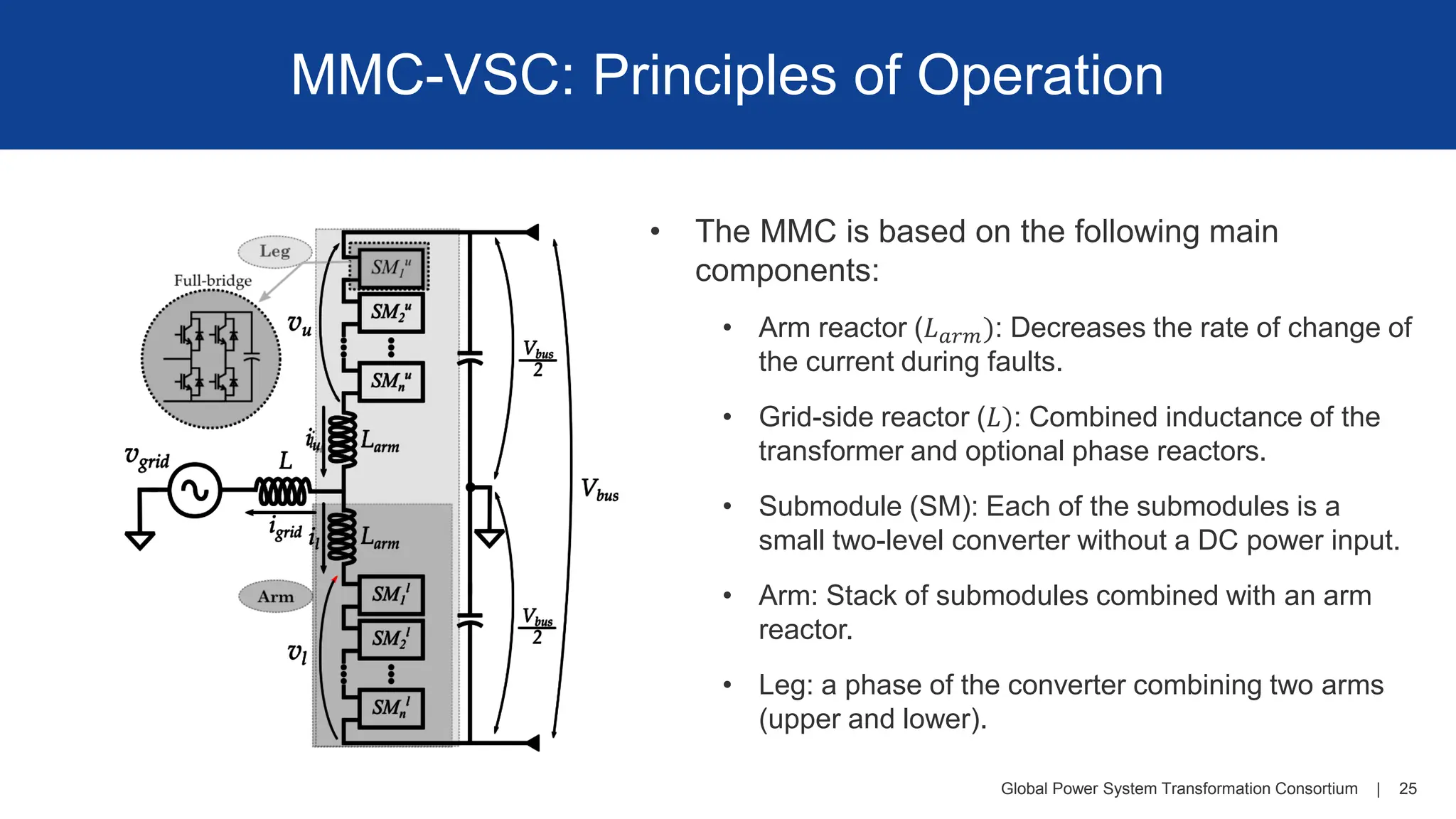
MMC-VSC: Principles of Operation
• The MMC is based on the following main
components:
• Arm reactor (𝐿𝑎𝑟𝑚): Decreases the rate of change of
the current during faults.
• Grid-side reactor (𝐿): Combined inductance of the
transformer and optional phase reactors.
• Submodule (SM): Each of the submodules is a
small two-level converter without a DC power input.
• Arm: Stack of submodules combined with an arm
reactor.
• Leg: a phase of the converter combining two arms
(upper and lower).
25.
Global Power SystemTransformation Consortium | 26
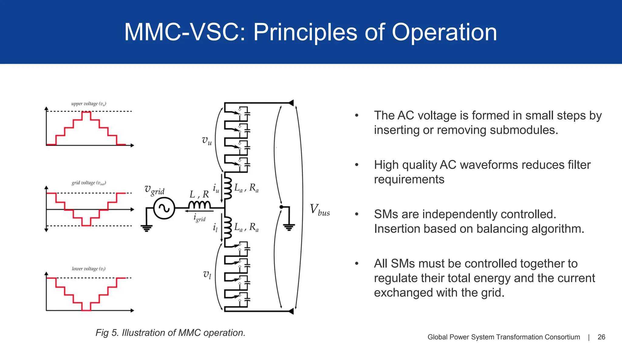
MMC-VSC: Principles of Operation
Fig 5. Illustration of MMC operation.
• The AC voltage is formed in small steps by
inserting or removing submodules.
• High quality AC waveforms reduces filter
requirements
• SMs are independently controlled.
Insertion based on balancing algorithm.
• All SMs must be controlled together to
regulate their total energy and the current
exchanged with the grid.
26.
Global Power SystemTransformation Consortium | 27
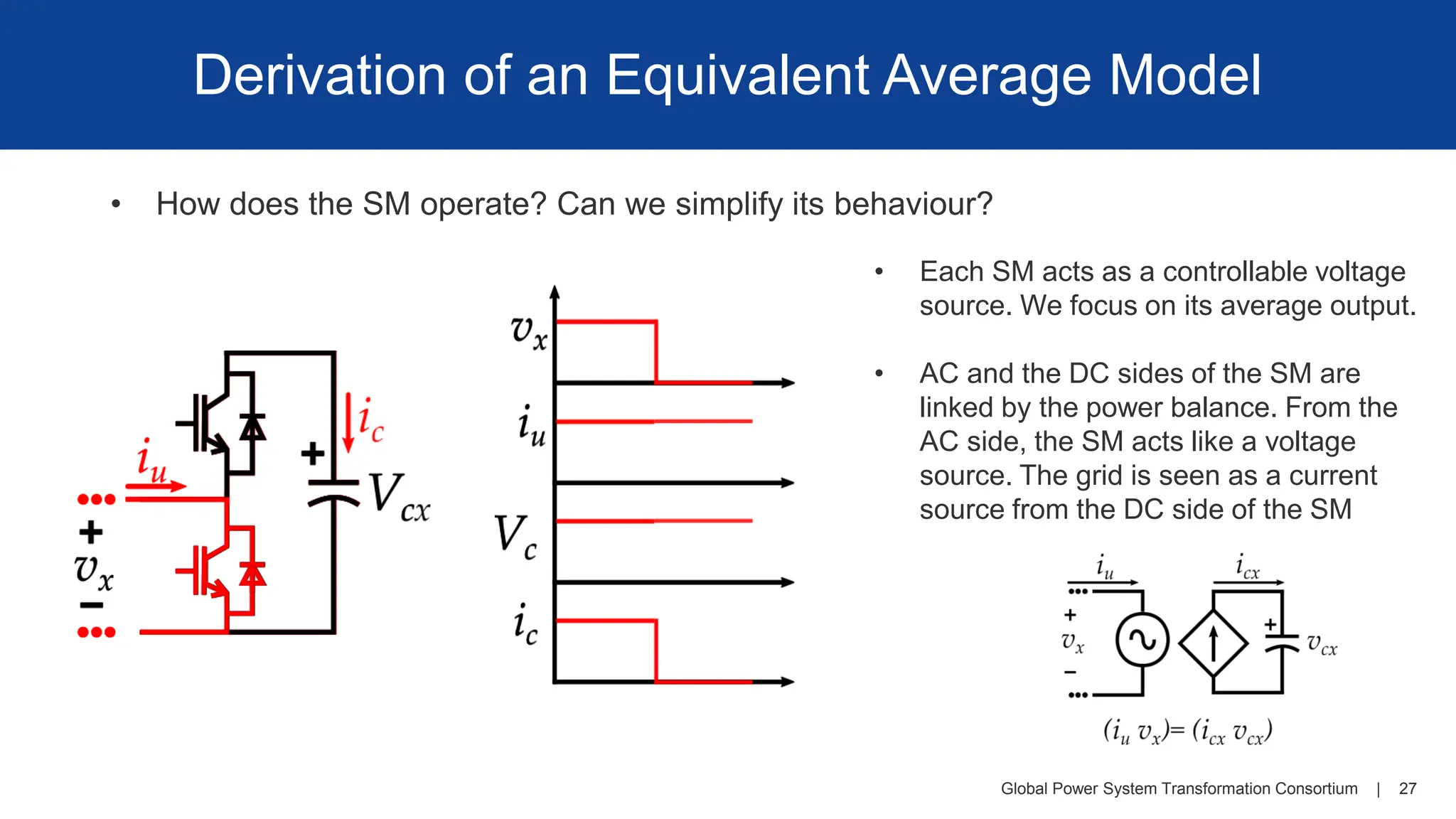
Derivation of an Equivalent Average Model
• How does the SM operate? Can we simplify its behaviour?
• Each SM acts as a controllable voltage
source. We focus on its average output.
• AC and the DC sides of the SM are
linked by the power balance. From the
AC side, the SM acts like a voltage
source. The grid is seen as a current
source from the DC side of the SM
27.
Global Power SystemTransformation Consortium | 28
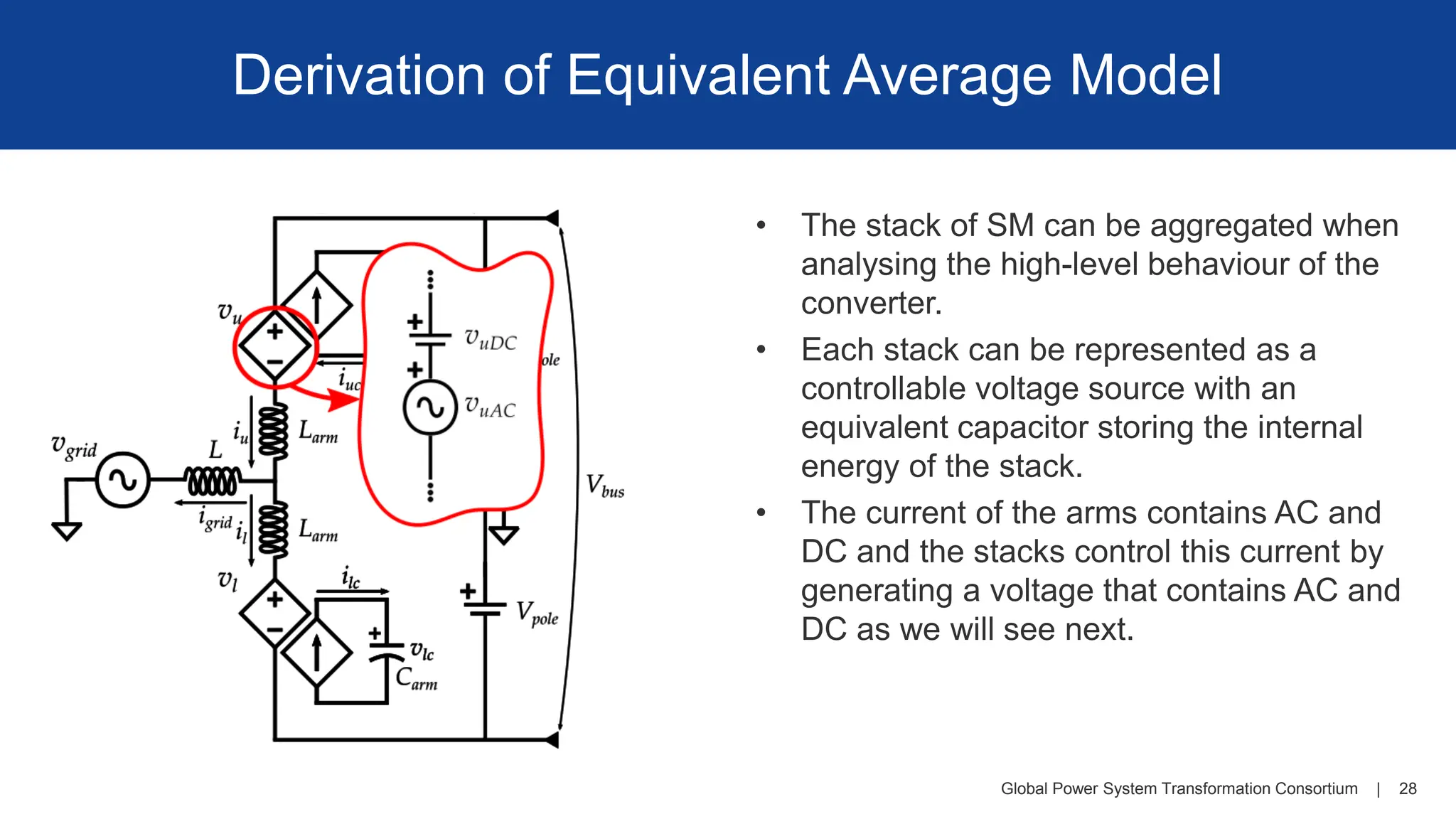
Derivation of Equivalent Average Model
• The stack of SM can be aggregated when
analysing the high-level behaviour of the
converter.
• Each stack can be represented as a
controllable voltage source with an
equivalent capacitor storing the internal
energy of the stack.
• The current of the arms contains AC and
DC and the stacks control this current by
generating a voltage that contains AC and
DC as we will see next.
28.
Global Power SystemTransformation Consortium | 29
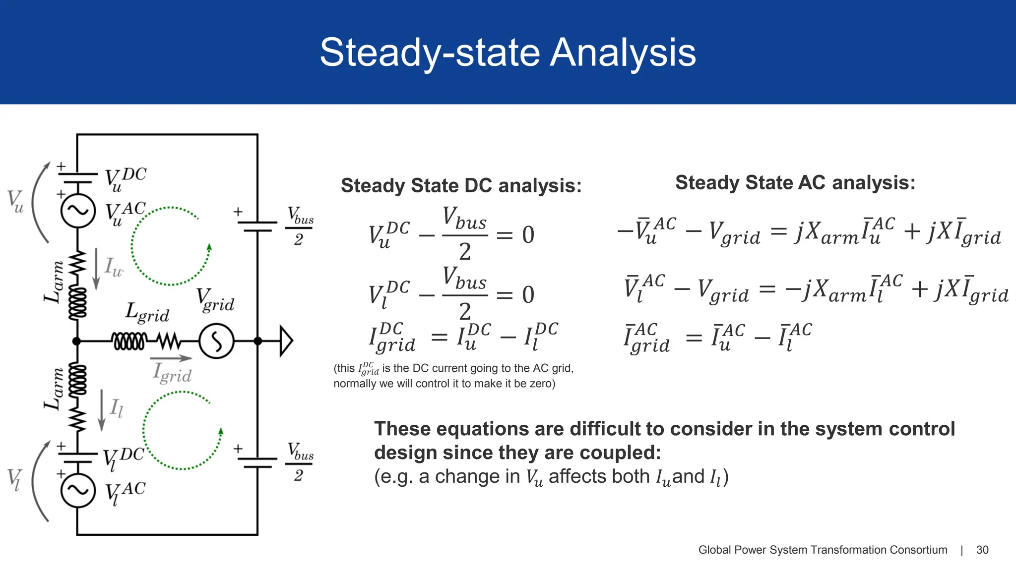
Steady-state Analysis
• Assumptions and approach:
• The stack energy dynamics are comparatively slower than the arm current dynamics, the two
are considered decoupled.
• First, we study the link between the voltages and the current circulating through the arms.
• Next, we look at the power exchanged by each element of the circuit to understand how the
internal energy of the converter can be controlled.
• The AC grid and the DC grid are simplified and considered to be ideal voltage sources.
29.
Global Power SystemTransformation Consortium | 30
Steady-state Analysis
𝑉
𝑢
𝐷𝐶
−
𝑉𝑏𝑢𝑠
2
= 0
𝑉𝑙
𝐷𝐶
−
𝑉𝑏𝑢𝑠
2
= 0
−ത
𝑉
𝑢
𝐴𝐶 − 𝑉𝑔𝑟𝑖𝑑 = 𝑗𝑋𝑎𝑟𝑚
ҧ
𝐼𝑢
𝐴𝐶 + 𝑗𝑋 ҧ
𝐼𝑔𝑟𝑖𝑑
ത
𝑉𝑙
𝐴𝐶
− 𝑉𝑔𝑟𝑖𝑑 = −𝑗𝑋𝑎𝑟𝑚
ҧ
𝐼𝑙
𝐴𝐶
+ 𝑗𝑋 ҧ
𝐼𝑔𝑟𝑖𝑑
ҧ
𝐼𝑔𝑟𝑖𝑑
𝐴𝐶
= ҧ
𝐼𝑢
𝐴𝐶 − ҧ
𝐼𝑙
𝐴𝐶
Steady State DC analysis: Steady State AC analysis:
𝐼𝑔𝑟𝑖𝑑
𝐷𝐶
= 𝐼𝑢
𝐷𝐶
− 𝐼𝑙
𝐷𝐶
These equations are difficult to consider in the system control
design since they are coupled:
(e.g. a change in 𝑉
𝑢 affects both 𝐼𝑢and 𝐼𝑙)
(this 𝐼𝑔𝑟𝑖𝑑
𝐷𝐶
is the DC current going to the AC grid,
normally we will control it to make it be zero)
30.
Global Power SystemTransformation Consortium | 31
Steady-state Analysis
𝑉
𝑥
𝑑𝑖𝑓𝑓
≜ −
1
2
𝑉
𝑥
𝑢 +
1
2
𝑉
𝑥
𝑙
𝑉
𝑥
𝑠𝑢𝑚
≜ 𝑉
𝑥
𝑢
+ 𝑉
𝑥
𝑙
𝑉
𝑥
𝑢 = −𝑉
𝑥
𝑑𝑖𝑓𝑓
+
1
2
𝑉
𝑥
𝑠𝑢𝑚
𝑉
𝑥
𝑙
= 𝑉
𝑥
𝑑𝑖𝑓𝑓
+
1
2
𝑉
𝑥
𝑠𝑢𝑚
𝐼𝑥
𝑠𝑢𝑚
≜
1
2
𝐼𝑥
𝑢
+
1
2
𝐼𝑥
𝑙
𝐼𝑥
𝐴𝐶 = 𝐼𝑥
𝑢 − 𝐼𝑥
𝑙
𝐼𝑥
𝑢
=
1
2
𝐼𝑥
𝐴𝐶
+ 𝐼𝑥
𝑠𝑢𝑚
𝐼𝑥
𝑙
= −
1
2
𝐼𝑥
𝐴𝐶
+ 𝐼𝑥
𝑠𝑢𝑚
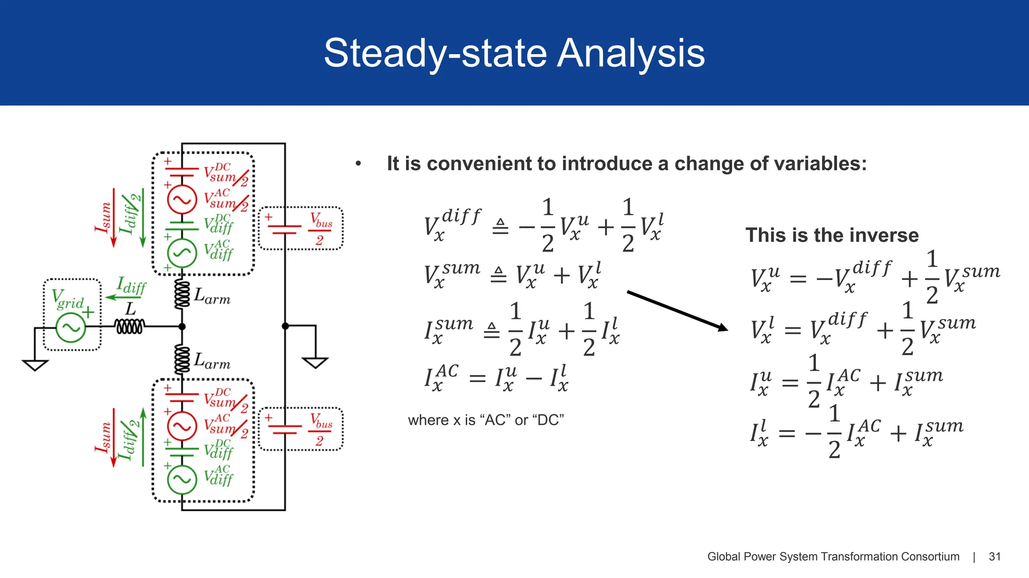
• It is convenient to introduce a change of variables:
This is the inverse
where x is “AC” or “DC”
31.
Global Power SystemTransformation Consortium | 32
Steady-state Analysis
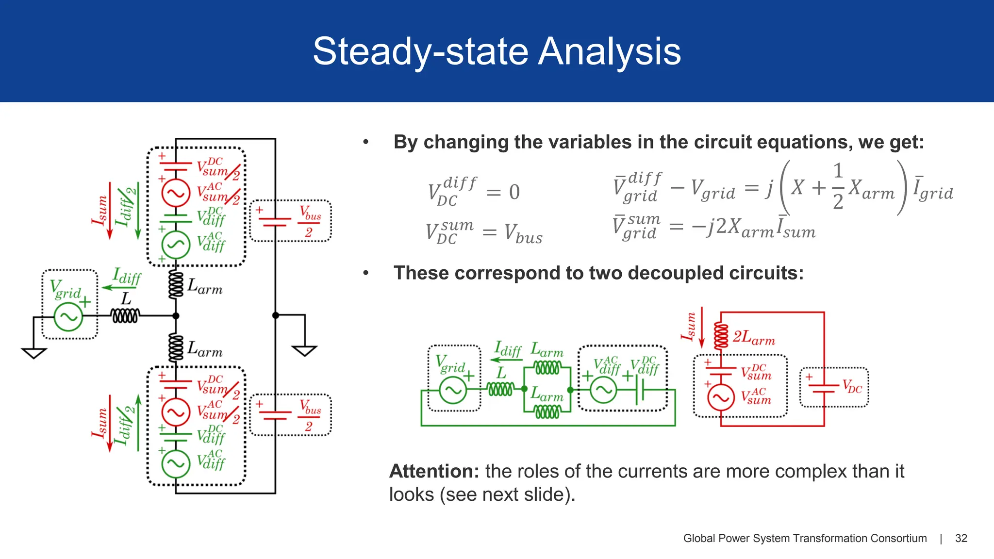
• These correspond to two decoupled circuits:
Attention: the roles of the currents are more complex than it
looks (see next slide).
• By changing the variables in the circuit equations, we get:
𝑉
𝐷𝐶
𝑑𝑖𝑓𝑓
= 0
𝑉𝐷𝐶
𝑠𝑢𝑚
= 𝑉𝑏𝑢𝑠
ത
𝑉𝑔𝑟𝑖𝑑
𝑑𝑖𝑓𝑓
− 𝑉𝑔𝑟𝑖𝑑 = 𝑗 𝑋 +
1
2
𝑋𝑎𝑟𝑚
ҧ
𝐼𝑔𝑟𝑖𝑑
ത
𝑉𝑔𝑟𝑖𝑑
𝑠𝑢𝑚
= −𝑗2𝑋𝑎𝑟𝑚
ҧ
𝐼𝑠𝑢𝑚
32.
Global Power SystemTransformation Consortium | 33
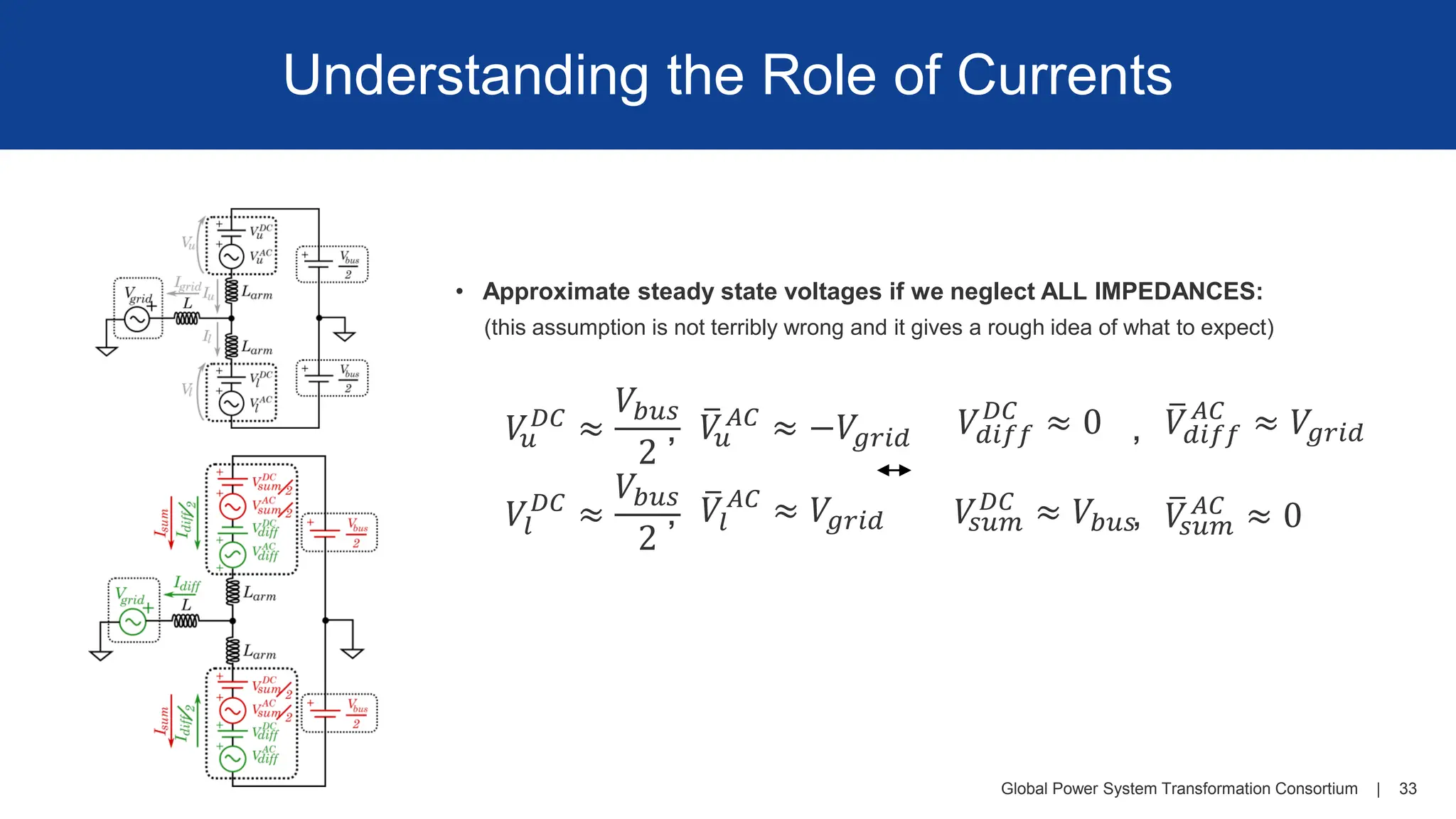
Understanding the Role of Currents
• Approximate steady state voltages if we neglect ALL IMPEDANCES:
𝑉
𝑢
𝐷𝐶 ≈
𝑉𝑏𝑢𝑠
2
𝑉𝑙
𝐷𝐶
≈
𝑉𝑏𝑢𝑠
2
ത
𝑉
𝑢
𝐴𝐶 ≈ −𝑉𝑔𝑟𝑖𝑑
ത
𝑉𝑙
𝐴𝐶
≈ 𝑉𝑔𝑟𝑖𝑑
,
,
𝑉𝑑𝑖𝑓𝑓
𝐷𝐶
≈ 0
𝑉
𝑠𝑢𝑚
𝐷𝐶 ≈ 𝑉𝑏𝑢𝑠
ത
𝑉𝑑𝑖𝑓𝑓
𝐴𝐶
≈ 𝑉𝑔𝑟𝑖𝑑
ത
𝑉
𝑠𝑢𝑚
𝐴𝐶 ≈ 0
,
,
(this assumption is not terribly wrong and it gives a rough idea of what to expect)
Global Power SystemTransformation Consortium | 35
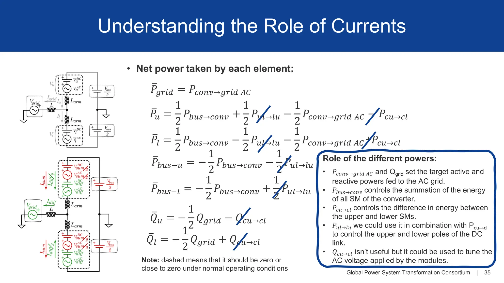
Understanding the Role of Currents
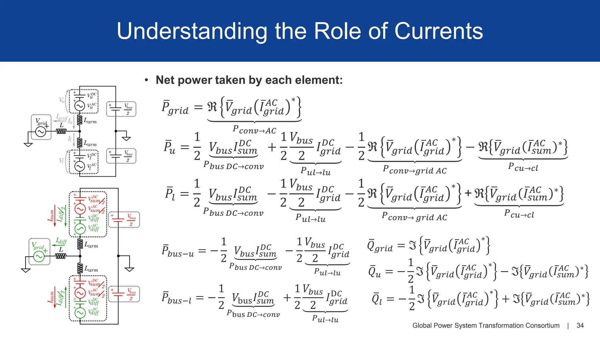
• Net power taken by each element:
ത
𝑃𝑢 =
1
2
𝑃𝑏𝑢𝑠→𝑐𝑜𝑛𝑣 +
1
2
𝑃𝑢𝑙→𝑙𝑢 −
1
2
𝑃𝑐𝑜𝑛𝑣→𝑔𝑟𝑖𝑑 𝐴𝐶 − 𝑃𝑐𝑢→𝑐𝑙
ത
𝑃𝑙 =
1
2
𝑃𝑏𝑢𝑠→𝑐𝑜𝑛𝑣 −
1
2
𝑃𝑢𝑙→𝑙𝑢 −
1
2
𝑃𝑐𝑜𝑛𝑣→𝑔𝑟𝑖𝑑 𝐴𝐶+𝑃𝑐𝑢→𝑐𝑙
ത
𝑃𝑏𝑢𝑠−𝑢 = −
1
2
𝑃𝑏𝑢𝑠→𝑐𝑜𝑛𝑣 −
1
2
𝑃𝑢𝑙→𝑙𝑢
ത
𝑃𝑏𝑢𝑠−𝑙 = −
1
2
𝑃𝑏𝑢𝑠→𝑐𝑜𝑛𝑣 +
1
2
𝑃𝑢𝑙→𝑙𝑢
ത
𝑄𝑢 = −
1
2
𝑄𝑔𝑟𝑖𝑑 − 𝑄𝑐𝑢→𝑐𝑙
ത
𝑄𝑙 = −
1
2
𝑄𝑔𝑟𝑖𝑑 + 𝑄𝑐𝑢→𝑐𝑙
ത
𝑃𝑔𝑟𝑖𝑑 = 𝑃𝑐𝑜𝑛𝑣→𝑔𝑟𝑖𝑑 𝐴𝐶
Role of the different powers:
• 𝑃𝑐𝑜𝑛𝑣→𝑔𝑟𝑖𝑑 𝐴𝐶 and Qgrid set the target active and
reactive powers fed to the AC grid.
• 𝑃𝑏𝑢𝑠→𝑐𝑜𝑛𝑣 controls the summation of the energy
of all SM of the converter.
• 𝑃𝑐𝑢→𝑐𝑙 controls the difference in energy between
the upper and lower SMs.
• 𝑃𝑢𝑙→𝑙𝑢 we could use it in combination with Pcu→cl
to control the upper and lower poles of the DC
link.
• 𝑄𝑐𝑢→𝑐𝑙 isn’t useful but it could be used to tune the
AC voltage applied by the modules.
Note: dashed means that it should be zero or
close to zero under normal operating conditions
35.
Global Power SystemTransformation Consortium | 36
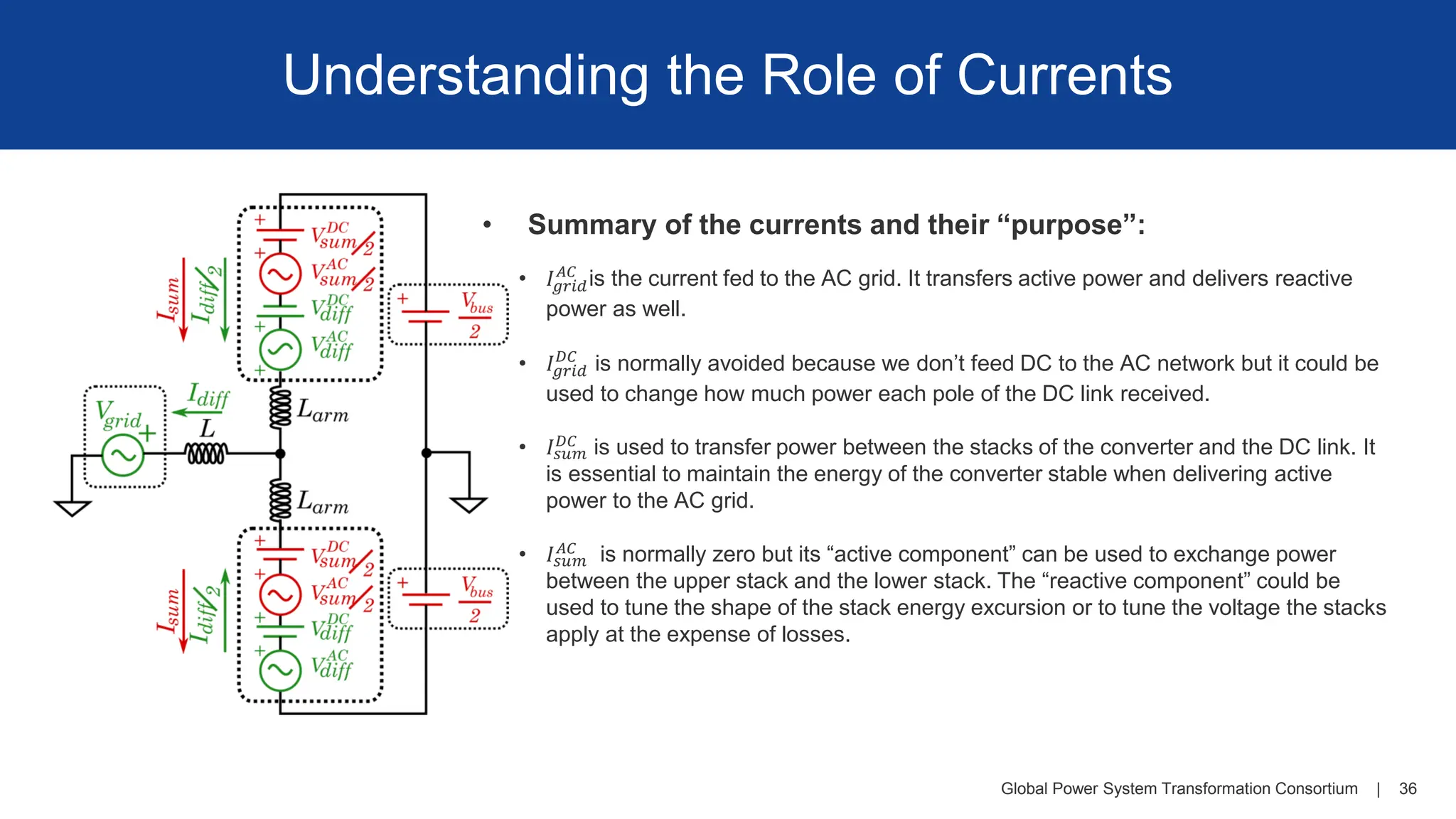
Understanding the Role of Currents
• Summary of the currents and their “purpose”:
• 𝐼𝑔𝑟𝑖𝑑
𝐴𝐶
is the current fed to the AC grid. It transfers active power and delivers reactive
power as well.
• 𝐼𝑔𝑟𝑖𝑑
𝐷𝐶
is normally avoided because we don’t feed DC to the AC network but it could be
used to change how much power each pole of the DC link received.
• 𝐼𝑠𝑢𝑚
𝐷𝐶
is used to transfer power between the stacks of the converter and the DC link. It
is essential to maintain the energy of the converter stable when delivering active
power to the AC grid.
• 𝐼𝑠𝑢𝑚
𝐴𝐶
is normally zero but its “active component” can be used to exchange power
between the upper stack and the lower stack. The “reactive component” could be
used to tune the shape of the stack energy excursion or to tune the voltage the stacks
apply at the expense of losses.
36.
Global Power SystemTransformation Consortium | 37
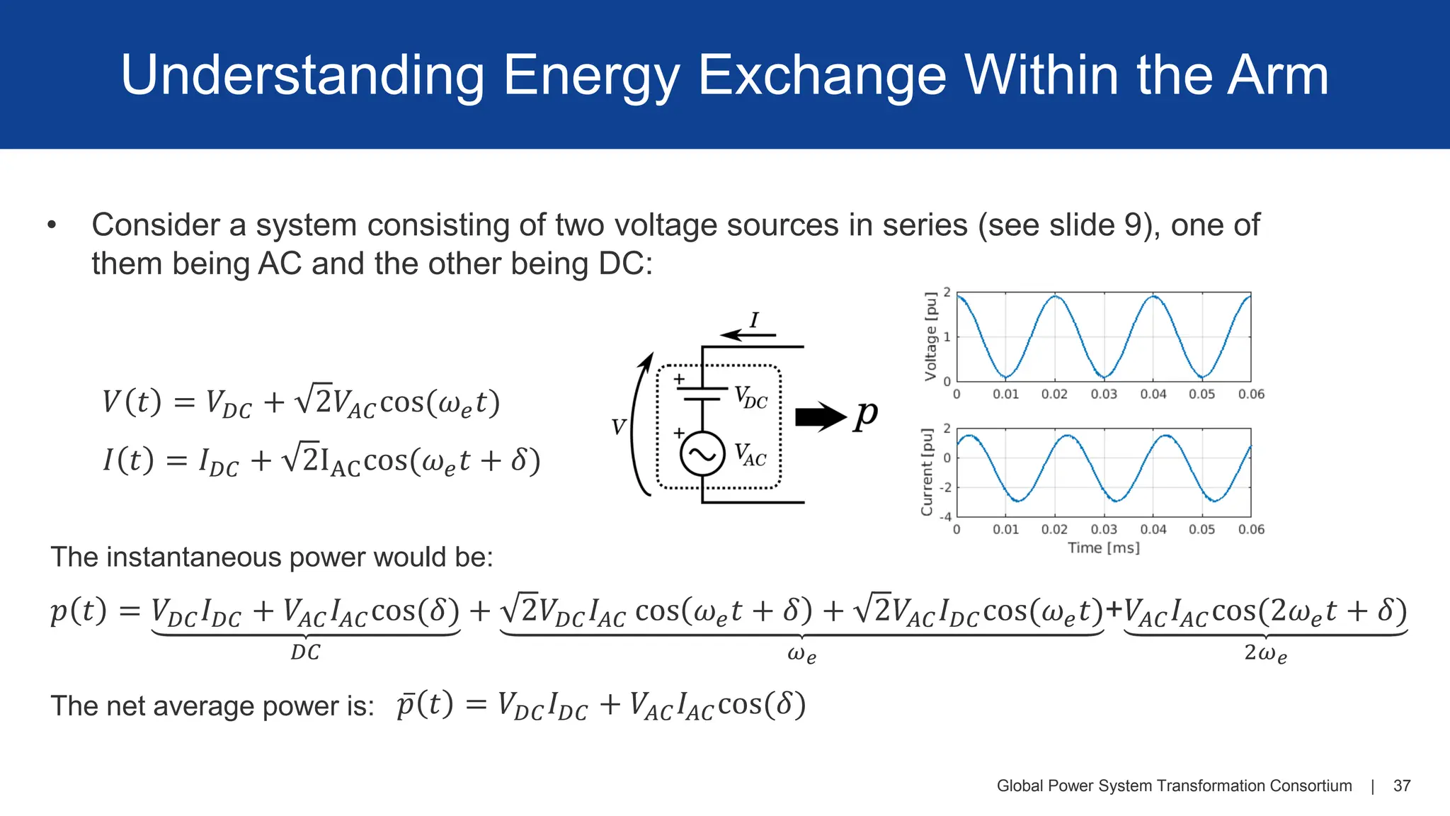
Understanding Energy Exchange Within the Arm
• Consider a system consisting of two voltage sources in series (see slide 9), one of
them being AC and the other being DC:
𝑉 𝑡 = 𝑉𝐷𝐶 + 2𝑉𝐴𝐶cos(𝜔𝑒𝑡)
𝐼 𝑡 = 𝐼𝐷𝐶 + 2IACcos(𝜔𝑒𝑡 + 𝛿)
𝑝 𝑡 = 𝑉𝐷𝐶𝐼𝐷𝐶 + 𝑉𝐴𝐶𝐼𝐴𝐶cos(𝛿)
𝐷𝐶
+ 2𝑉𝐷𝐶𝐼𝐴𝐶 cos 𝜔𝑒𝑡 + 𝛿 + 2𝑉𝐴𝐶𝐼𝐷𝐶cos(𝜔𝑒𝑡)
𝜔𝑒
+𝑉𝐴𝐶𝐼𝐴𝐶cos(2𝜔𝑒𝑡 + 𝛿)
2𝜔𝑒
ҧ
𝑝 𝑡 = 𝑉𝐷𝐶𝐼𝐷𝐶 + 𝑉𝐴𝐶𝐼𝐴𝐶cos(𝛿)
The instantaneous power would be:
The net average power is:
37.
Global Power SystemTransformation Consortium | 38
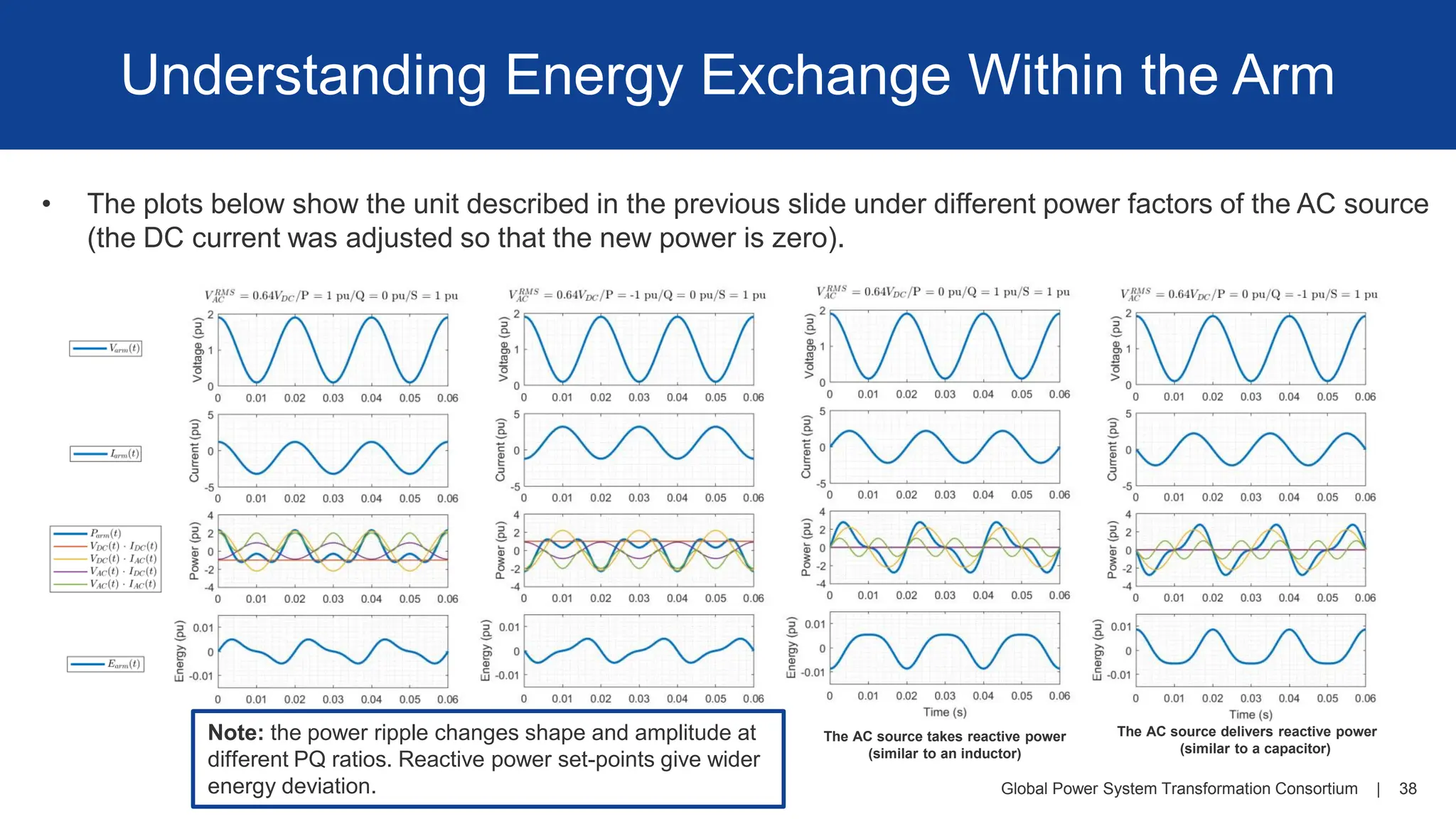
Understanding Energy Exchange Within the Arm
AC source takes active power
(similar to a resistor)
The AC source delivers active power
The AC source takes reactive power
(similar to an inductor)
The AC source delivers reactive power
(similar to a capacitor)
• The plots below show the unit described in the previous slide under different power factors of the AC source
(the DC current was adjusted so that the new power is zero).
Note: the power ripple changes shape and amplitude at
different PQ ratios. Reactive power set-points give wider
energy deviation.
38.
Global Power SystemTransformation Consortium | 39
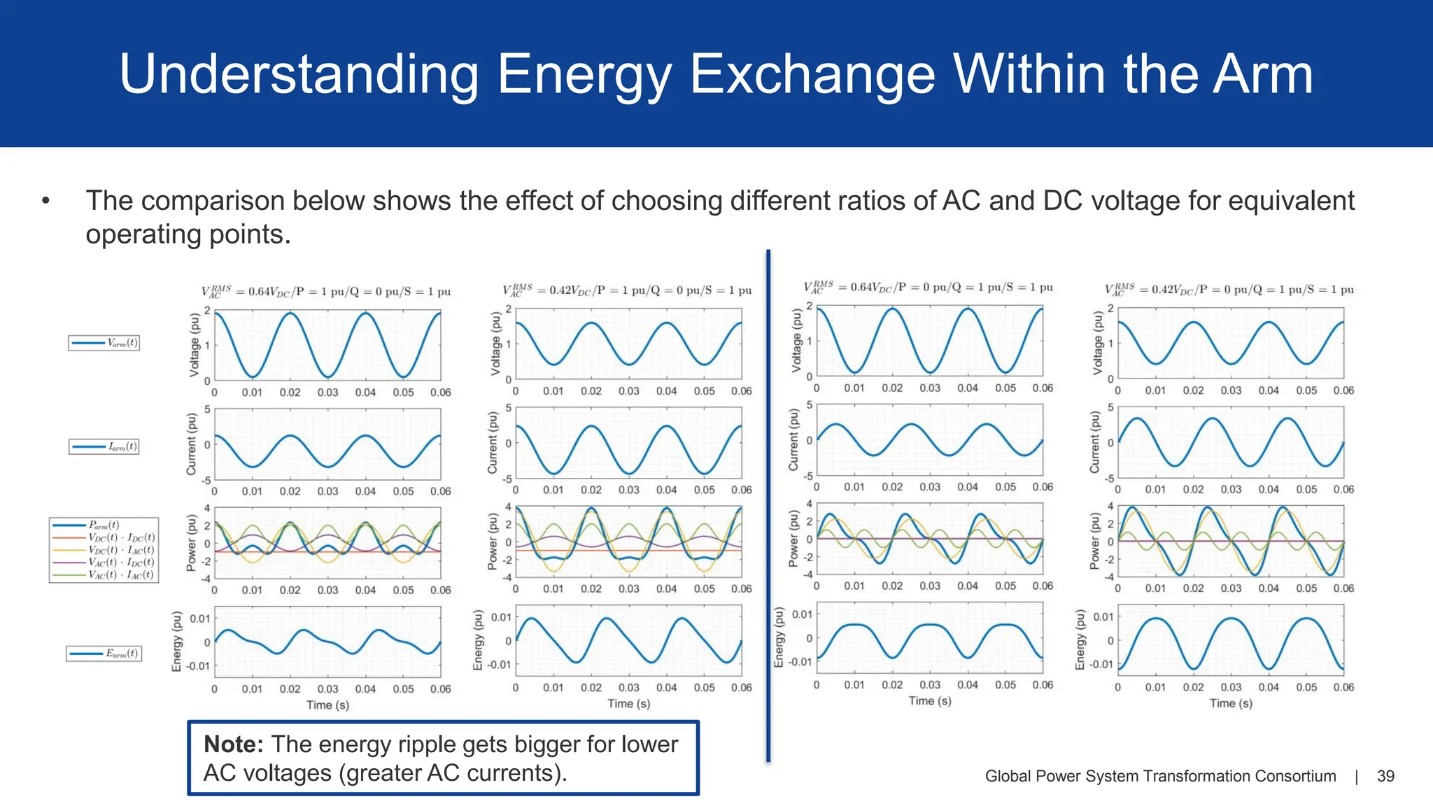
Understanding Energy Exchange Within the Arm
• The comparison below shows the effect of choosing different ratios of AC and DC voltage for equivalent
operating points.
Note: The energy ripple gets bigger for lower
AC voltages (greater AC currents).
39.
Global Power SystemTransformation Consortium | 40
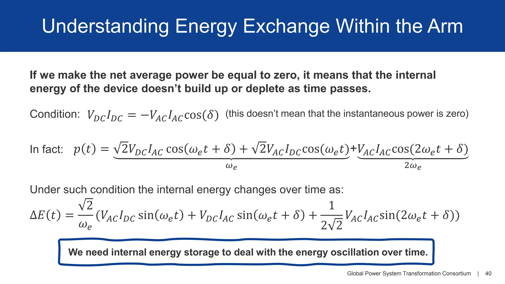
Understanding Energy Exchange Within the Arm
If we make the net average power be equal to zero, it means that the internal
energy of the device doesn’t build up or deplete as time passes.
𝑉𝐷𝐶𝐼𝐷𝐶 = −𝑉𝐴𝐶𝐼𝐴𝐶cos(𝛿)
𝑝 𝑡 = 2𝑉𝐷𝐶𝐼𝐴𝐶 cos 𝜔𝑒𝑡 + 𝛿 + 2𝑉𝐴𝐶𝐼𝐷𝐶cos(𝜔𝑒𝑡)
𝜔𝑒
+𝑉𝐴𝐶𝐼𝐴𝐶cos(2𝜔𝑒𝑡 + 𝛿)
2𝜔𝑒
In fact:
Δ𝐸 𝑡 =
2
𝜔𝑒
(𝑉𝐴𝐶𝐼𝐷𝐶 sin 𝜔𝑒𝑡 + 𝑉𝐷𝐶𝐼𝐴𝐶 sin 𝜔𝑒𝑡 + 𝛿 +
1
2 2
𝑉𝐴𝐶𝐼𝐴𝐶sin(2𝜔𝑒𝑡 + 𝛿))
Under such condition the internal energy changes over time as:
Condition: (this doesn’t mean that the instantaneous power is zero)
We need internal energy storage to deal with the energy oscillation over time.
40.
Global Power SystemTransformation Consortium | 41
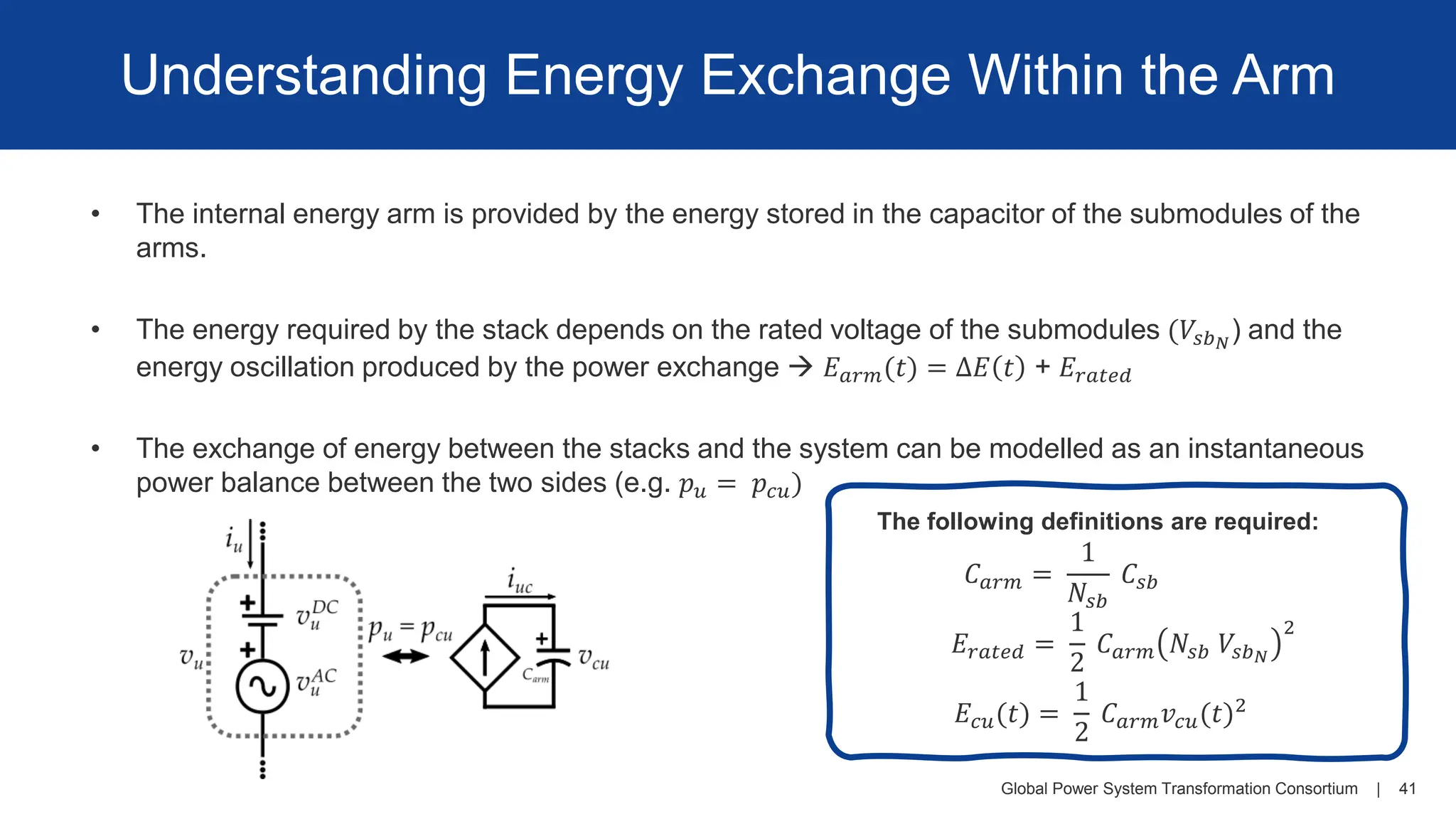
Understanding Energy Exchange Within the Arm
• The internal energy arm is provided by the energy stored in the capacitor of the submodules of the
arms.
• The energy required by the stack depends on the rated voltage of the submodules (𝑉𝑠𝑏𝑁
) and the
energy oscillation produced by the power exchange → 𝐸𝑎𝑟𝑚(𝑡) = Δ𝐸 𝑡 + 𝐸𝑟𝑎𝑡𝑒𝑑
• The exchange of energy between the stacks and the system can be modelled as an instantaneous
power balance between the two sides (e.g. 𝑝𝑢 = 𝑝𝑐𝑢)
𝐸𝑟𝑎𝑡𝑒𝑑 =
1
2
𝐶𝑎𝑟𝑚 𝑁𝑠𝑏 𝑉𝑠𝑏𝑁
2
The following definitions are required:
𝐶𝑎𝑟𝑚 =
1
𝑁𝑠𝑏
𝐶𝑠𝑏
𝐸𝑐𝑢(𝑡) =
1
2
𝐶𝑎𝑟𝑚𝑣𝑐𝑢(𝑡)2
41.
Global Power SystemTransformation Consortium | 42
Summary
• Things we’ve seen in this session:
• Context overview of the HVDC technology
• Review of evolution of VSC up to the MMC topology
• The principles of operation of the MMC
• Steady-state equations of power and energy when combining AC and DC in the
same circuit
• The role of the different currents within the MMC
• How the MMC exchanges power between its AC and DC sides
• Considerations about output voltage rating and internal energy of the converter
• Steady-state analysis of a practical single-phase MMC.
DISCLAIMER
This work wasproduced by Dr. Adria Junyent-Ferre
and Dr. Joan Marc Rodriguez-Bernuz under the G-
PST. This work is not for commercial purposes. The
views expressed in this material do not necessarily
represent the views of the Department of Energy or
the U.S. Government, or any agency thereof, including
Imperial College London or Imperial Consultants.
RESOURCES
• Visit the G-PST website.
• Learn more about the G-PST’s Foundational Workforce
Development Pillar.
• Visit the Imperial College London website.
|
Connect with the G-PST on
social media to stay up to date
on Women in PST, research,
free trainings, and curriculum.
44.
Contact Our Team
•G-PST’s Workforce Development Pillar Leads: Tim Green at t.green@imperial.ac.uk
and Balarko Chaudhuri at b.chaudhuri@imperial.ac.uk
• Course Instructor: Dr. Adria Junyent-Ferre at ajunyent@ic.ac.uk and Dr. Joan Marc
Rodriguez-Bernuz at j.rodriguez15@ic.ac.uk


![Global Power System Transformation Consortium | 10
Basic VSC: Inner Regulator
[1] Sigurd Skogestad and Ian Postlethwaite. 2005. Multivariable Feedback Control:
Analysis and Design. John Wiley & Sons, Inc., Hoboken, NJ, USA.
• Different techniques can be used to design the
inner regulator (e.g. PI, PR, ℋ∞,etc.). For instance,
a PI can be used to track a DC reference, which
can be easily tuned following the Internal Model
Control (IMC) technique. The inner regulator can
be tuned based on the plant and desired system
time-constant 𝜏. [1]
If we use a PI as a regulator: 𝐾 𝑠 = 𝐾𝑝 +
𝐾𝐼
𝑠
The closed-loop function becomes: 𝑇 𝑠 =
𝐼𝑜𝑢𝑡(𝑠)
𝐼𝑜𝑢𝑡
∗
(𝑠)
=
𝐺 𝑠 𝐾(𝑠)
1 + 𝐺 𝑠 𝐾(𝑠)
≈
1
𝜏𝑠 + 1
with the following PI gains... 𝐾𝑝 =
𝐿
𝜏
and 𝐾𝐼 =
𝑅
𝜏
Simulation example: 𝐿 = 100 uH, 𝑅= 1 𝑚Ω, 𝑉𝑏𝑎𝑡 = 50 V, 𝑉𝑏𝑢𝑠 = 100 V. 𝜏 = 10 ms.
𝐾𝑝 = 0.01 and 𝐾𝐼 = 0.1. The input reference 𝐼𝑜𝑢𝑡
∗
does a step change from 0 to 10 at
time 0.1 s. (see file: inner_regulator_example.mo)
Closed-loop time
response show 63% of
final value is achieved
10 ms after change.](https://image.slidesharecdn.com/modular-multilevel-converter-high-voltage-direct-current-mmc-hvdc-course-session-1-250630211219-30728be3/75/Modular-Multilevel-Converter-High-Voltage-Direct-Current-MMC-HVDC-Course-Session-1-pdf-10-2048.jpg)
![Global Power System Transformation Consortium | 12
Basic VSC: Outer Regulator
The gains are set to give a specific maximum transient error
of Δ𝑉𝑏𝑢𝑠
𝑀𝐴𝑋
for a sudden change of the current fed to the DC
bus of Δ𝐼𝑠𝑜𝑢𝑟𝑐𝑒
𝑀𝐴𝑋
.
[1] Sigurd Skogestad and Ian Postlethwaite. 2005. Multivariable Feedback Control:
Analysis and Design. John Wiley & Sons, Inc., Hoboken, NJ, USA.
Gains for specified peak transient error:
𝐾𝑃 = −
𝟐𝚫𝑰𝑠𝑜𝑢𝑟𝑐𝑒
𝑴𝑨𝑿
𝒆𝚫𝑽𝑏𝑢𝑠
𝑴𝑨𝑿
𝐾𝐼 = −
𝑲𝑷
𝟐
𝟒𝑪
Figure: Outer regulator response to a step-change of the current
fed to the DC bus and to a change of Vbus reference.
Δ𝑉𝑏𝑢𝑠
𝑀𝐴𝑋](https://image.slidesharecdn.com/modular-multilevel-converter-high-voltage-direct-current-mmc-hvdc-course-session-1-250630211219-30728be3/75/Modular-Multilevel-Converter-High-Voltage-Direct-Current-MMC-HVDC-Course-Session-1-pdf-12-2048.jpg)