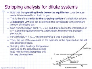
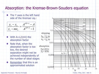
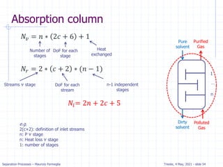
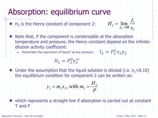
The document presents an overview of absorption and stripping processes in separation operations, highlighting the fundamentals, analytical solutions, and various methodologies such as McCabe-Thiele. Absorption involves the uptake of a gas by a liquid solvent while stripping is the reverse process, and both can operate in equilibrium columns. Key concepts include solubility, energy balances, and the relationships between phases using equations like Henry’s law and the Kremser equation.

![Separation Processes – Maurizio Fermeglia Trieste, 4 May, 2021 - slide 19
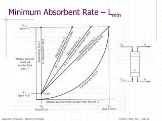
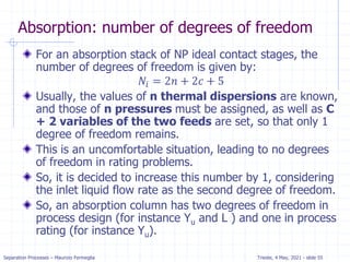
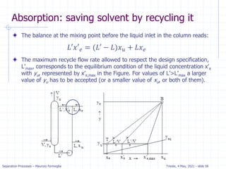
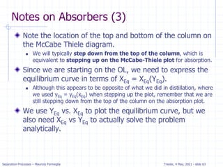
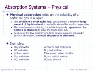
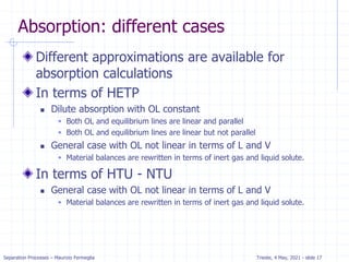
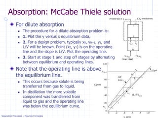
Absorption: McCabe Thiele solution
For dilute absorption
We can assume that L and V are both constant, and the
operating line on a McCabe-Thiele diagram will be
straight.
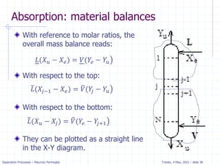
Using the mass balance envelope around the top of the
absorption column shown in Figure, we can write the
solute mass balance for constant L and V.
Solving for yj+1 we obtain the equation for the McCabe-
Thiele operating line.
With slope L/V and y-intercept [y1 – (L/V)x0].
All possible passing streams with compositions (xj, yj+1)
must lie on the operating line.
This includes the two streams at the top of the absorber
(x0, y1) and the two streams at the bottom of the
absorber (xN, yN+1).
𝑦𝑖+1𝑉 + 𝑥0𝐿 = 𝑦1 + 𝑥𝑦𝐿
𝑦𝑖+1 =
𝐿
𝑉
𝑥𝑗 + [𝑦1 −
𝐿
𝑉
𝑥0]](https://image.slidesharecdn.com/01absorption-240726141554-738ed240/85/Modelling-absorption-column-for-engineers-18-320.jpg)
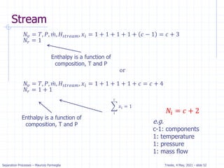
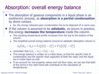
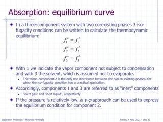
![Separation Processes – Maurizio Fermeglia Trieste, 4 May, 2021 - slide 23
c
a
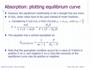
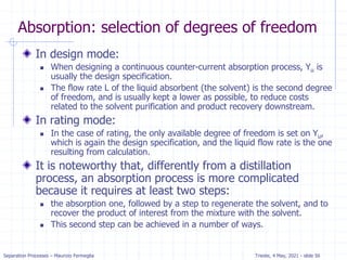
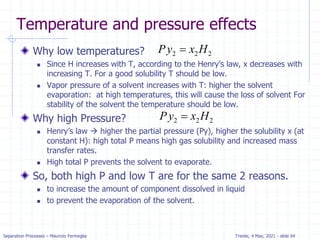
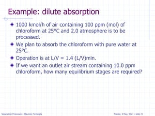
Example: dilute absorption
Equation of OL is valid when j=N.
Solving for xN with x0=0 we get.
xN= (yN+1-y1) / (L/V) =
(100-10) / 133 = .68 ppm
Five equilibrium stages are
more than sufficient.
If desired, we can estimate a
fractional number of
equilibrium contacts:
𝑦𝑖+1 =
𝐿
𝑉
𝑥𝑗 + [𝑦1 −
𝐿
𝑉
𝑥0]
Fraction = (distance from OL to xN)/
(distance from OL to equilibrium line)
= (distance a to b)/(distance a to c)
= 0.08/0.2 = 0.4
Thus, we need 4.4 equilibrium contacts.](https://image.slidesharecdn.com/01absorption-240726141554-738ed240/85/Modelling-absorption-column-for-engineers-22-320.jpg)
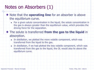
![Separation Processes – Maurizio Fermeglia Trieste, 4 May, 2021 - slide 24
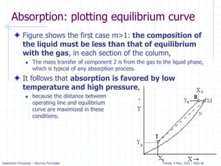
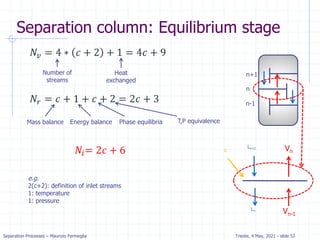
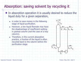
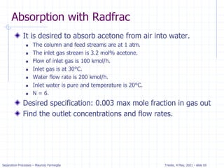
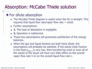
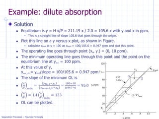
Stripping analysis for dilute systems
Since stripping is very similar to absorption we expect the
method to be similar.
The mass balance for the column is the same and the OL is the same:
For stripping we know x0, xN, yN+1, and L/V. Since (xN, yN+1) is a point on
the operating line, we can plot the operating line and step off stages.
𝑦𝑖+1 =
𝐿
𝑉
𝑥𝑗 + [𝑦1 −
𝐿
𝑉
𝑥0]](https://image.slidesharecdn.com/01absorption-240726141554-738ed240/85/Modelling-absorption-column-for-engineers-23-320.jpg)