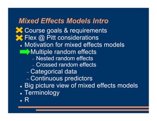
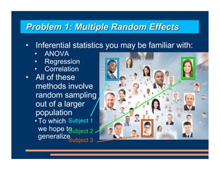
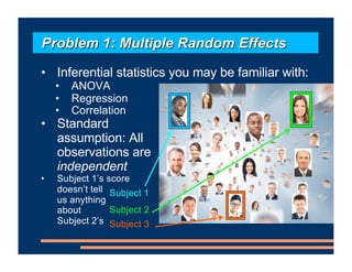
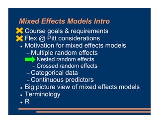
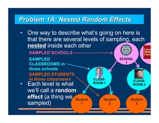
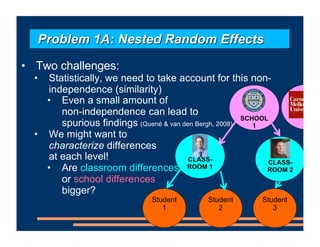
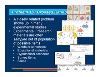
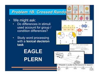
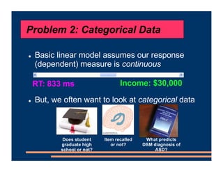
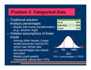
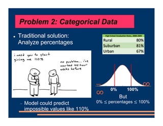
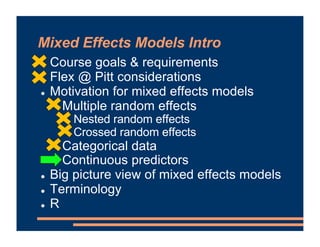
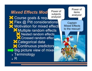
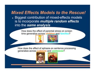
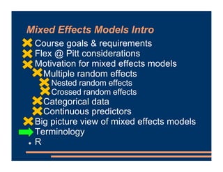
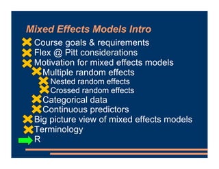
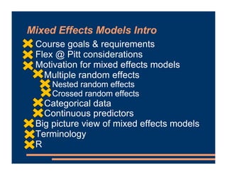
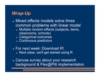
This document discusses an upcoming course on using mixed effects models in psychology. The course will cover applying mixed effects models to common research designs, fitting models in R, and addressing issues that arise. Mixed effects models are motivated by research designs involving multiple random effects, nested random effects, crossed random effects, categorical dependent variables, and continuous predictors. Accounting for these complex sampling procedures and non-independent observations is important for making valid statistical inferences.
This document provides information about a business course, including that there will be class on Labor Day and lab materials are available on Canvas. It discusses fixed effects in models and how to include them in R scripts. Predicted values from models are covered, along with using residuals to detect outliers and interpreting interactions between variables in models. The document provides examples of adding interaction terms to model formulas and interpreting the results.
This document provides an introduction to logit models for categorical outcomes. It discusses how logit models use a logistic link function to model the log odds of categorical outcomes as a linear combination of predictors while accounting for random effects. Key points covered include probabilities, odds, the logit transformation, interpreting model parameters, and implementing logit models in R using the glmer() function from the lme4 package.
R allows users to perform calculations, analyze data, and create visualizations through commands and functions. This document discusses R basics including commands, functions, arguments, reading in data from files, and performing descriptive statistics. Key points covered include using the pipe operator (%)>% to chain multiple functions together, loading and summarizing data, and obtaining descriptive statistics for single and multiple variables as well as grouped variables.
This document provides information and examples related to interpreting interaction effects in statistical models. It begins with an overview of how to interpret numerical interaction terms and then provides several examples of interactions between variables and their interpretation. These include examples involving intrinsic motivation and autonomy on learning, number of choices and maximizing strategy on satisfaction, language proficiency and word frequency on translation accuracy, and more. It then shifts to discussing model comparison, including nested models, hypothesis testing using likelihood ratio tests, and comparing models.
This document provides an overview of data processing techniques in R, including filtering, mutating, and working with different variable types. It discusses using filter() to subset data frames based on logical criteria, saving filtered data to new data frames. It also covers using mutate() to create new variables and recode existing ones. The if_else() function and applying conditional logic when assigning values is explained. The document concludes with a brief overview of variable types in R like numeric, character, and factor, as well as functions for converting between types and examples of built-in and package functions for analysis.
The document discusses introducing mixed effects models. It focuses on fixed effects, which are the effects of interest. This week covers sample datasets, theoretical models, fitting models in R, and interpreting parameters like slopes and intercepts. The sample dataset examines factors like newcomers and experience that influence how long teams take to assemble phones. The document uses this example to demonstrate key steps in modeling fixed effects, such as estimating slopes, intercepts, and conducting hypothesis tests on parameters.
The document discusses introducing random slopes to multilevel models. Random slopes allow the relationship between a predictor variable (like tutor hours) to vary across levels (like schools). This accounts for differences in how effective an intervention may be depending on context. The notation for random slopes models is presented, with classroom and student models nested within school-level models. Implementing random slopes helps address non-independence of observations and better estimate variability.
There are a few potential issues with modeling the data this way:
1. Students are nested within classrooms. A student's outcomes may be more similar to others in their classroom compared to students in other classrooms, due to shared classroom factors. This violates the independence assumption of ordinary least squares regression.
2. Classroom-level factors like teacher quality are not included in the model but likely influence student outcomes. Failing to account for these could lead to omitted variable bias.
3. The error terms for students within the same classroom may not be independent as assumed, since classroom factors induce correlation.
To properly account for the nested data structure, we need to model the classroom as a second level in a multilevel
Mixed Effects Models - Centering and TransformationsScott Fraundorf
This document provides information about analyzing a dataset called numerosity that contains reaction time (RT) data from a dot counting task and self-reported math anxiety ratings. It discusses centering the numerosity (number of dots) and anxiety variables, including mean centering, centering around other values, and the difference between grand-mean and cluster-mean centering. It also covers transforming the numerosity variable using logarithms due to the non-linear relationship with RT. The goal is to build mixed effects models to examine the effects of numerosity and anxiety on RT.
1. Post-hoc comparisons allow testing differences between individual levels or cells in an experiment after fitting a linear mixed effects model. The Tukey test, available via the emmeans package, corrects for multiple comparisons.
2. Estimated marginal means (EMMs) report what cell means would be if covariates were equal across conditions, providing a hypothetical adjustment. EMMs can be compared to test effects averaging over other variables.
3. Both post-hoc comparisons and EMMs require fitting an appropriate linear mixed effects model first before making inferences about condition differences.
This document discusses empirical logit models. It begins by clarifying logit models, which use a logit link function to model binary dependent variables. It then discusses Poisson regression models. The document notes that empirical logit can be used to model low-frequency events like errors or rare outcomes that may have probabilities close to 0. Empirical logit makes extreme probabilities less extreme by adding 0.5 to the numerator and denominator when calculating the logit. It concludes by discussing how to implement empirical logit models using the psycholing package in R.
Mixed Effects Models - Crossed Random EffectsScott Fraundorf
This document discusses crossed random effects analysis using an experimental dataset measuring response times for students learning English naming words. The dataset includes 60 subjects presented with 49 words each, with measurements of years of study and word frequency as variables of interest. It describes fitting a linear mixed effects model with random intercepts for subject and word to account for non-independence of observations. It also discusses joining additional word frequency data from another file and adding word frequency as a fixed effect. Finally, it introduces the concepts of between-subjects and within-subjects variables to determine what random slopes may be relevant.
Mixed Effects Models - Signal Detection TheoryScott Fraundorf
Signal detection theory provides a framework for analyzing categorical judgments by distinguishing between sensitivity and response bias. Sensitivity refers to the ability to discriminate between signal and noise, such as detecting whether sentence pairs are the same color. Response bias reflects the overall tendency to respond in a certain category, such as a propensity to judge sentences as grammatical. Signal detection theory models allow researchers to separately measure how experimental manipulations influence these components of performance.
This document discusses effect size and how to establish causality in longitudinal data analysis. It begins by reviewing autocorrelation and how to account for it in mixed effects models. It then discusses cross-lagged models, where including lags of variables can help determine whether A causes B or B causes A. Establishing causality further requires showing the relationship is directional by testing models in both directions. The document provides an example using a diary study to show that emotional support attempts cause increased warmth, not vice versa. It also discusses how effect size compares to statistical significance and how to interpret the size of different effects.
The "Instrumental Variables" webinar, presented by Peter Lance, was the fifth and final webinar in a series of discussions on the popular MEASURE Evaluation manual, How Do We Know If a Program Made a Difference? A Guide to Statistical Methods for Program Impact Evaluation.
Application of Weighted Least Squares Regression in Forecastingpaperpublications3
Abstract: This work models the loss of properties from fire outbreak in Ogun State using Simple Weighted Least Square Regression. The study covers (secondary) data on fire outbreak and monetary value of properties loss across the twenty (20) Local Government Areas of Ogun state for the year 2010. Data collected were analyzed electronically using SPSS 21.0. Results from the analysis reveal that there is a very strong positive relationship between the number of fire outbreak and the loss of properties; this relationship is significant. Fire outbreak exerts significant influence on loss of properties and it accounts for approximately 91.2% of the loss of properties in the state.
This document provides an overview of key concepts in structural equation modeling (SEM) including:
1) Path diagrams are used to represent structural equations and the relationships between latent and observed variables.
2) SEM analyzes the variance/covariance matrix of observed variables rather than raw data. Maximum likelihood estimation is used to estimate model parameters by maximizing the likelihood of the sample data.
3) Model identification, fit, and constraints are important concepts. A model must be over-identified to yield a likelihood value for assessing fit. Parameter constraints can be used to make a just-identified model over-identified.
This document provides information about independent samples t-tests and dependent/paired samples t-tests. It explains that independent samples t-tests are used to compare two independent groups, while dependent samples t-tests are used to compare observations within a single group. The key steps for each test are outlined, including stating hypotheses, calculating the test statistic, determining critical values, and making conclusions. Examples are provided to demonstrate how to perform the tests by hand and using SPSS.
This document discusses regression models, path models, and the output from AMOS software when conducting structural equation modeling (SEM). Regression models only include observed variables and assume independents are measured without error. Path models allow independents to be both causes and effects, and allow for error terms on endogenous variables. The AMOS output provides standardized and unstandardized regression weights, significance tests, and fit indexes to evaluate how well the specified model fits the sample data.
Standard deviationnormal distributionshowBiologyIB
This tutorial provides information about the normal curve and normal distributions. It discusses key characteristics of the normal curve including that most values fall in the middle and fewer values fall at the extremes. It also discusses how to calculate percentages of values that fall within a certain number of standard deviations from the mean. Additional topics covered include using z-scores to standardize values, types of normal distributions that vary in spread, and how data is not always normally distributed if skewed to one side.
El documento discute la regresión particionada, donde las variables explicativas se dividen en dos subconjuntos. Explica que los estimadores de los coeficientes no cambian si se considera la partición de las variables, y que los resultados de la proyección no cambian. También muestra que el estimador del segundo subconjunto de variables depende de los residuales de la regresión del primer subconjunto.
Potential Solutions to the Fundamental Problem of Causal Inference: An OverviewEconomic Research Forum
Ragui Assaad- University of Minnesota
Caroline Krafft- ST. Catherine University
ERF Training on Applied Micro-Econometrics and Public Policy Evaluation
Cairo, Egypt July 25-27, 2016
www.erf.org.eg
Este documento describe las características generales de los lenguajes de simulación de sistemas discretos y sus ventajas. Explica que estos lenguajes automatizan muchas funciones necesarias como la generación de números aleatorios, control del flujo del tiempo y recolección de datos. También proveen un ambiente natural para modelar simulaciones y son fáciles de usar, alcanzando algunos de ellos la ingeniería de software. El documento lista algunos ejemplos de lenguajes de simulación como MIDAS, DYSAC, DSL y GPSS
This document discusses including level-2 variables in multilevel models. It explains that level-2 variables characterize groups (like classrooms) and are invariant within groups. An example adds the variable "TeacherTheory" to characterize teachers' mindset and explain differences between classrooms. This reduces unexplained classroom variance but does not change the level-1 model or residuals. Cross-level interactions like the effect of a student's mindset depending on their teacher's mindset can also be added. Including level-2 variables provides more information about group differences but does not alter the basic multilevel structure.
JiTT - Blended Learning Across the Academy - Teaching Prof. Tech - Oct 2015Jeff Loats
This document summarizes a presentation on implementing Just-in-Time Teaching (JiTT), a blended learning strategy. The presentation provides an overview of JiTT, shares data from courses that have used JiTT showing increased student preparation and performance, and offers recommendations for getting started with JiTT. Sample JiTT questions are also presented along with student responses to demonstrate how the strategy works.
This document discusses issues that can arise with missing or incomplete data in statistical models. It covers several types of problems, including rank deficiency caused by linear dependencies between predictors, and incomplete designs where certain combinations of factor levels are not represented in the data. It also discusses different patterns of missing data and how the mechanism that led to certain data points being missing (missing completely at random, missing at random, or missing not at random) impacts which techniques are appropriate for handling the missing values, such as casewise deletion, listwise deletion, or imputation methods. Examples using the lmer function in R and a dataset on cortisol levels are provided to illustrate these concepts.
This document provides an introduction to research methods. It discusses why understanding research methods is important for interdisciplinary researchers and outlines different types of research such as quantitative, qualitative, and mixed methods. It also discusses how to experimentally measure learning, including within and between subjects designs. The document provides examples of how to design studies to obtain desired results and addresses important statistical concepts like independent and dependent variables. It raises considerations for survey design and cautions about assumptions of parametric statistics.
Generalizability in fMRI, fast and slowTal Yarkoni
- The document discusses issues around generalizability in fMRI research and proposes strategies for "fast" versus "slow" generalization.
- It notes that most findings in neuroimaging are only interesting if they generalize broadly, but that statistical models must support desired inferences about new stimuli or subjects.
- The document advocates treating factors like subjects and stimuli as random effects to support generalization, and using large stimulus samples to avoid overgeneralizing findings. It suggests both modeling approaches (e.g. random effects) and study design (e.g. more stimuli/subjects) can help researchers generalize more appropriately.
Jeff Loats - Scholarly Teaching - TLD, Feb 2015Jeff Loats
The document discusses the importance of teaching as a social science and using evidence-based teaching methods. It notes that expertise in a discipline can lead one to underestimate their knowledge of teaching skills, while a lack of teaching expertise can inflate one's beliefs. Effective teaching requires applying rigorous scholarship to pedagogy and choosing methods informed by empirical research showing the benefits of active learning, preparation, feedback, and iterative learning. Studies have found evidence-based teaching significantly improves student learning compared to traditional lectures.
1 University of Wollongong School of Psychol.docxdorishigh
1
University of Wollongong
School of Psychology
PSYC 250: Quantitative Methods in
Psychology
Assignment 2
INSTRUCTIONS:
This assignment is graded out of 30 marks, and it is worth 21% of the overall grade for the
subject. It is to be submitted by Fri 25 September 5.00pm.
This is an individual assignment, and all the work must be entirely your own.
You must show all working to gain full marks. Round the final answers to two decimal
places. Marks may be deducted for disorganized work.
For questions requiring a written answer, keep your answers to within 50 words each. The
only exception is when you need to provide report a statistical analysis in APA format. Write
your answers clearly with in blue or black ink.
Submit your answers in hardcopy (either hand-written or printed out). You must attach an
official signed declaration cover page, or else your assignment will not be graded.
Furthermore, you must submit an electronic file (see below).
2
ELECTRONIC FILE SUBMISSION INSTRUCTIONS:
Create ONE ELECTRONIC FILE that contains your written answers to the following
questions in Assignment 2, below:
Question 1d (APA style results section)
Question 2e (APA style results section)
Question 3 (written definition of what is an interaction effect is, and description of the
interaction in the given scenario)
HOW: In the Moodle site for PSY250, Click on the link that says "Assignment 2
(TurnItIn)". Click on the "My Submissions" tab. Next to "Submission Title", enter
"Assignment 2". Click the small box next to the statement "I confirm that this submission is
my own work...". Then, next to "File to Submit", click on "Browse..." and select the
document that you want to upload. Then click on "Add Submission".
DUE DATE: The same deadline as the hardcopy Assignment 2 applies. Your Assignment
will be considered late if either the hardcopy OR the electronic file are late.
NOTE: Although you are not required to turn in any other portion of the assignment through
TurnItIn, your responses to the other parts of the Assignment should still be your own work,
in your own words.
3
Question 1 [11 marks]
In obsessive-compulsive disorder (OCD) patients often display irrational compulsive behavior
such as repeated hand-washing, flicking light-switches on and off or compulsively counting
things. These behaviours are generally performed by the patient to stop obsessive negative
thoughts
A clinical psychologist examined the efficacy of 3 different treatments for OCD:
Family therapy – which promotes understanding of the disorder within the patients’ family
group.
Cognitive Behaviour therapy - which addresses obsessive thought patterns
Attending a support group with other patients with OCD.
Twenty-one patients with OCD were randomly assigned to one of three treatment conditions.
After six months the number ...
This document outlines the syllabus for an introductory statistics course over summer session I in 2015. The course will cover topics including describing and summarizing data, probability, random sampling, estimating population parameters, significance tests, contingency tables, simple linear regression and correlation. It will meet Monday through Friday from 12:30-2:30 pm. The instructor is Nicholas Thorne and office hours are Tuesdays and Wednesdays from 10:30-12:30 pm. The primary textbook is Statistics for People Who Hate Statistics. There will be homework assignments, in-class assignments, two exams, and a total of 500 possible points for the class between these components.
The exam for this psychology unit will be 1 hour long and test three sections of the material. Students will have to answer three questions testing their knowledge of experiments, correlations, observations, or self-reports. The exam questions will ask students to discuss the strengths and weaknesses of a piece of research, interpret data, and design their own study.
Timed tests cause early onset of math anxiety in students according to research. Studies have shown that students experience stress on timed math tests that they do not experience on untimed tests of the same material. Even young students in 1st and 2nd grade can experience math anxiety, and their levels do not correlate with factors like grade level, reading ability, or family income. Brain imaging has revealed that students who feel panicky about math show increased activity in areas associated with fear and decreased activity in areas involved in problem solving. Timed tests require retrieving math facts from working memory, and higher math anxiety reduces the available working memory. While timed tests are used with good intentions, the evidence suggests they should be reconsidered given the widespread issues
This document provides strategies for teaching undergraduate students to solve physics problems. It discusses using cooperative group problem solving based on cognitive apprenticeship as an effective method. Key aspects include using context-rich problems that require an organized problem-solving framework, structuring student groups to provide peer coaching, and gradually reducing scaffolding such as limiting equations and providing grading guidance. The goal is to help students develop expert-like problem-solving skills.
1. Experimental design refers to how experiments are structured in order to ensure validity and reliability of results.
2. There are several types of experimental designs including true experimental, quasi-experimental, pre-experimental, ex post facto, and factorial designs.
3. True experimental designs use random assignment and control/experimental groups to establish causation. Quasi-experimental designs lack random assignment so can only suggest relationships between variables. Ex post facto designs study pre-existing groups and cannot prove causation. Factorial designs study effects of multiple independent variables.
This lab focuses on testing hypotheses about adolescent sexual behavior. The activities include reading literature about adolescents who committed sexual abuse, observing and interpreting anonymized real-world data on adolescents who did or did not commit abuse, developing a hypothesis to test using the data, graphically depicting the results and drawing conclusions using descriptive statistics, and presenting the results. The objectives are to identify factors that may predict sexually offending behaviors according to literature, articulate a research question and methodology to test using the data, and describe possible assessment or treatment approaches based on conclusions. Homework includes preparing for an in-class discussion and completing a reflection.
This document discusses designing quality open-ended tasks in mathematics. It provides two methods for creating open-ended questions: working backwards from a closed question and adapting a standard question. Good open-ended tasks engage all students, allow for diverse responses, and enable teachers to interact with and understand students' mathematical thinking. When planning open-ended tasks, teachers should consider the mathematical focus, clarity of the task, and include enabling and extending prompts. High quality student responses systematically consider all possible solutions and make connections across mathematical concepts.
Common Shortcomings in SE Experiments (ICSE'14 Doctoral Symposium Keynote)Natalia Juristo
This document discusses best practices for designing and analyzing software engineering experiments. It outlines key aspects of experiments such as definition, operationalization of variables, experimental design, implementation, analysis, and publication. Regarding design, it emphasizes controlling irrelevant variables through randomization and blocking. It provides an example experiment comparing model-driven development to traditional development. The document stresses iterative design to address validity threats and importance of statistical power.
This document outlines a workshop on assessment and feedback approaches. It discusses challenges with current assessment practices, such as an over-reliance on summative assessments and a lack of formative feedback. It then presents the TESTA (Transforming the Experience of Students Through Assessment) approach, which aims to address these issues by taking a whole-program approach to balancing summative and low-stakes formative assessments and improving feedback practices. The workshop involves examining assessment data, discussing challenges, and learning TESTA principles for improving assessment design and student experience.
This document discusses defining and selecting a research problem. It provides several criteria for selecting a good problem, including novelty, importance, interest to the researcher, and feasibility. A research problem refers to a difficulty a researcher wants to solve in a theoretical or practical context. A problem statement should clearly outline the problem in 1-2 sentences using the 5Ws (who, what, when, where, why). It should also address how the problem will be studied and tested. Characteristics of a good problem include being empirically testable and examining relationships between variables. Defining the problem sets the direction and goals of the study.
Oral Exams and Rubrics: An introductionJoAnn MIller
1. The document provides guidance on creating rubrics to assess oral exams in a simple, fair, and rapid manner.
2. It describes organizing oral exams with role cards and allowing students to leave once finished. It also presents a 5-point scale to grade accuracy and fluency.
3. Specific instructions are given for conducting two parts of the oral exam - a roleplay graded for accuracy, and a roleplay with the teacher graded for fluency. Sample roleplay situations are also included.
4. Additional information is provided on defining expectations through rubrics, the difference between holistic and analytic rubrics, and the importance of
Similar to Mixed Effects Models - Introduction (20)
🔥🔥🔥🔥🔥🔥🔥🔥🔥
إضغ بين إيديكم من أقوى الملازم التي صممتها
ملزمة تشريح الجهاز الهيكلي (نظري 3)
💀💀💀💀💀💀💀💀💀💀
تتميز هذهِ الملزمة بعِدة مُميزات :
1- مُترجمة ترجمة تُناسب جميع المستويات
2- تحتوي على 78 رسم توضيحي لكل كلمة موجودة بالملزمة (لكل كلمة !!!!)
#فهم_ماكو_درخ
3- دقة الكتابة والصور عالية جداً جداً جداً
4- هُنالك بعض المعلومات تم توضيحها بشكل تفصيلي جداً (تُعتبر لدى الطالب أو الطالبة بإنها معلومات مُبهمة ومع ذلك تم توضيح هذهِ المعلومات المُبهمة بشكل تفصيلي جداً
5- الملزمة تشرح نفسها ب نفسها بس تكلك تعال اقراني
6- تحتوي الملزمة في اول سلايد على خارطة تتضمن جميع تفرُعات معلومات الجهاز الهيكلي المذكورة في هذهِ الملزمة
واخيراً هذهِ الملزمة حلالٌ عليكم وإتمنى منكم إن تدعولي بالخير والصحة والعافية فقط
كل التوفيق زملائي وزميلاتي ، زميلكم محمد الذهبي 💊💊
🔥🔥🔥🔥🔥🔥🔥🔥🔥
Gender and Mental Health - Counselling and Family Therapy Applications and In...PsychoTech Services
A proprietary approach developed by bringing together the best of learning theories from Psychology, design principles from the world of visualization, and pedagogical methods from over a decade of training experience, that enables you to: Learn better, faster!
How Barcodes Can Be Leveraged Within Odoo 17Celine George
In this presentation, we will explore how barcodes can be leveraged within Odoo 17 to streamline our manufacturing processes. We will cover the configuration steps, how to utilize barcodes in different manufacturing scenarios, and the overall benefits of implementing this technology.
Elevate Your Nonprofit's Online Presence_ A Guide to Effective SEO Strategies...TechSoup
Whether you're new to SEO or looking to refine your existing strategies, this webinar will provide you with actionable insights and practical tips to elevate your nonprofit's online presence.
Level 3 NCEA - NZ: A Nation In the Making 1872 - 1900 SML.pptHenry Hollis
The History of NZ 1870-1900.
Making of a Nation.
From the NZ Wars to Liberals,
Richard Seddon, George Grey,
Social Laboratory, New Zealand,
Confiscations, Kotahitanga, Kingitanga, Parliament, Suffrage, Repudiation, Economic Change, Agriculture, Gold Mining, Timber, Flax, Sheep, Dairying,
This presentation was provided by Rebecca Benner, Ph.D., of the American Society of Anesthesiologists, for the second session of NISO's 2024 Training Series "DEIA in the Scholarly Landscape." Session Two: 'Expanding Pathways to Publishing Careers,' was held June 13, 2024.
1. Using Mixed Effects Models in
Psychology
Scott Fraundorf
sfraundo@pitt.edu
Zoom office hours:
Wed 11-12, or by appointment
2. Mixed Effects Models Intro
! Course goals & requirements
! Flex @ Pitt considerations
! Motivation for mixed effects models
- Multiple random effects
- Nested random effects
- Crossed random effects
- Categorical data
- Continuous predictors
! Big picture view of mixed effects models
! Terminology
! R
3. Course Goals
! We will:
- Understand form of mixed effects models
- Apply mixed effects models to common
designs in psychology and related fields (e.g.,
factorial experiments, educational
interventions, longitudinal studies)
- Fit mixed effects models in R using lme4
- Diagnose and address common issues in
using mixed effects models
! We won’t:
- Cover algorithms used by software to compute
mixed effects models
4. Course Requirements
! We’ll be fitting models in R
! Free & runs on basically any computer
! Next week, will cover basics of using R
5. Mixed Effects Models Intro
! Course goals & requirements
! Flex @ Pitt considerations
! Motivation for mixed effects models
- Multiple random effects
- Nested random effects
- Crossed random effects
- Categorical data
- Continuous predictors
! Big picture view of mixed effects models
! Terminology
! R
7. Mixed Effects Models Intro
! Course goals & requirements
! Flex @ Pitt considerations
! Motivation for mixed effects models
- Multiple random effects
- Nested random effects
- Crossed random effects
- Categorical data
- Continuous predictors
! Big picture view of mixed effects models
! Terminology
! R
8. • Inferential statistics you may be familiar with:
• ANOVA
• Regression
• Correlation
• All of these
methods involve
random sampling
out of a larger
population
• To which
we hope to
generalize
Problem 1: Multiple Random Effects
Subject 1
Subject 2
Subject 3
9. • Inferential statistics you may be familiar with:
• ANOVA
• Regression
• Correlation
• Standard
assumption: All
observations are
independent
• Subject 1’s score
doesn’t tell
us anything
about
Subject 2’s
Problem 1: Multiple Random Effects
Subject 1
Subject 2
Subject 3
10. • Independence
assumption is fair if
we randomly sample
1 person at a time
• e.g., you recruit 40
undergrads from the
Psychology Subject
Pool
• But maybe this
isn’t all we should
be doing… (Henrich
et al., 2010, Nature)
Problem 1: Multiple Random Effects
11. • Important assumption!
• Does testing benefit
learning of biology?
Problem 1: Multiple Random Effects
Section A
n=50
Practice
quizzes
Section C
n=50
Practice
quizzes
Section B
n=50
Restudy
Section D
n=50
Restudy
12. • Impressive if 100
separate people who
did practice tests
learned better than
100 people who
reread the textbook
• Not so impressive
when we realize these
aren’t fully
independent
• Need to account
for differences in
instructor, time of
day
•
Problem 1: Multiple Random Effects
13. Mixed Effects Models Intro
! Course goals & requirements
! Flex @ Pitt considerations
! Motivation for mixed effects models
- Multiple random effects
- Nested random effects
- Crossed random effects
- Categorical data
- Continuous predictors
! Big picture view of mixed effects models
! Terminology
! R
14. • But many sensible, informative research
designs involve more complex sampling
procedures
• Example: Sampling
multiple children
from the same family
• Kids from the
same family
will be more
similar
• a/k/a clustering
Child 2
FAMILY 1 FAMILY 2
Child 3
Child 1
Problem 1A: Nested Random Effects
15. • But many sensible, informative research
designs involve more complex sampling
procedures
• Or: Two people in
a relationship
• Or any other
small group
(work teams,
experimentally
formed groups,
etc.)
COUPLE 1
Problem 1A: Nested Random Effects
16. • But many sensible, informative research
designs involve more complex sampling
procedures
• Or: A longitudinal study
• Each person is sampled multiple times
• Some characteristics don’t change over time—or
don’t change much
Problem 1A: Nested Random Effects
17. • But many sensible, informative research
designs involve more complex sampling
procedures
• Or: Kids in classrooms in schools
• Kids from the
same school will be
more similar
• Kids in same classroom
will be even more
similar!
Problem 1A: Nested Random Effects
Student
2
CLASS-
ROOM 1
Student
3
Student
1
CLASS-
ROOM 2
SCHOOL
1
18. • One way to describe what’s going on here is
that there are several levels of sampling, each
nested inside each other
• Each level is what
we’ll call a random
effect (a thing we
sampled)
Problem 1A: Nested Random Effects
SAMPLED SCHOOLS
SAMPLED
CLASSROOMS in
those schools
SAMPLED STUDENTS
in those classrooms
Student
2
CLASS-
ROOM 1
Student
3
Student
1
CLASS-
ROOM 2
SCHOOL
1
19. • Two challenges:
• Statistically, we need to take account for this non-
independence (similarity)
• Even a small amount of
non-independence can lead to
spurious findings (Quené & van den Bergh, 2008)
• We might want to
characterize differences
at each level!
• Are classroom differences
or school differences
bigger?
Problem 1A: Nested Random Effects
Student
2
CLASS-
ROOM 1
Student
3
Student
1
CLASS-
ROOM 2
SCHOOL
1
20. Mixed Effects Models Intro
! Course goals & requirements
! Flex @ Pitt considerations
! Motivation for mixed effects models
- Multiple random effects
- Nested random effects
- Crossed random effects
- Categorical data
- Continuous predictors
! Big picture view of mixed effects models
! Terminology
! R
21. Problem 1B: Crossed Random Effects
• A closely related problem
shows up in many
experimental studies
• Experimental / research
materials are often
sampled out of population
of possible items
• Words or sentences
• Educational materials
• Hypothetical scenarios
• Survey items
• Faces
22. Problem 1B: Crossed Random Effects
• We might ask:
• Do differences in stimuli
used account for group /
condition differences?
• Study word processing
with a lexical decision
task
EAGLE
PLERN
23. Problem 1B: Crossed Random Effects
• We might ask:
• Do differences in stimuli
used account for group /
condition differences?
• e.g., Maybe easier
vocab words used in
one condition
Unprimed
Primed
EAGLE
PENGUIN
EAGLE
MONKEY
24. Problem 1B: Crossed Random Effects
• We might ask:
• Do differences in stimuli
used account for group /
condition differences?
• Do our results generalize
to the population of all
relevant items?
• All vocab words
• All fictional resumes
• All questionnaire items
that measure
extraversion
• All faces
25. Problem 1B: Crossed Random Effects
• Again, we are sampling
two things—subjects
and items
• Arrangement is slightly
different because each
subject gets each item
• Crossed random effects
• Still, problem is that we
have multiple random
effects (things being
sampled)
Subject 1 Subject 2
EAGLE MONKEY
26. • Robustness across stimuli has been a major
concern in psycholinguistics for a long time
Problem 1B: Crossed Random Effects
27. • Robustness across stimuli has been a major
concern in psycholinguistics for a long time
• If you are doing research related to language
processing, you’ll be expected to address this
• (But stats classes don’t always teach you how)
• Now growing interest in other fields, too
Problem 1B: Crossed Random Effects
28. • Robustness across stimuli has been a major
concern in psycholinguistics for a long time
• If you are doing research related to language
processing, you’ll be expected to address this
• (But stats classes don’t always teach you how)
• Now growing interest in other fields, too
• Be a statistical pioneer!
• Test generalization across items
• Characterize variability
• Increase power (more likely to
detect a significant effect)
Problem 1B: Crossed Random Effects
29. F1(1,3) = 18.31, p < .05
F2(1,4) = 22.45, p < .01
Problem 1B: Crossed Random Effects
! OLD ANOVA solution:
Do 2 analyses
! Subjects analysis:
Compare each subject
(averaging over all of
the items)
! Does the effect
generalize across
subjects?
! Items analysis:
Compare each item
(averaging over all of
the subjects)
! Does the effect
generalize across items?
SUBJECT ANALYSIS
ITEM ANALYSIS
30. Problem 1B: Crossed Random Effects
! OLD ANOVA solution:
Do 2 analyses
! Subjects analysis
! Items analysis
! Problem: We now have
2 different sets of
results. Might conflict!
! Possible to combine
them with min F’, but
not widely used
F1(1,3) = 18.31, p < .05
F2(1,4) = 22.45, p < .01
SUBJECT ANALYSIS
ITEM ANALYSIS
31. Mixed Effects Models Intro
! Course goals & requirements
! Flex @ Pitt considerations
! Motivation for mixed effects models
- Multiple random effects
- Nested random effects
- Crossed random effects
- Categorical data
- Continuous predictors
! Big picture view of mixed effects models
! Terminology
! R
32. Problem 2: Categorical Data
! Basic linear model assumes our response
(dependent) measure is continuous
! But, we often want to look at categorical data
RT: 833 ms
Does student
graduate high
school or not?
Item recalled
or not?
What predicts
DSM diagnosis of
ASD?
Income: $30,000
33. Problem One: Categorical Data
! Traditional solution:
Analyze percentages
! Maybe with some transformation
(e.g., arcsine, logit)
! Violates assumptions of linear
model
- Among other issues: Linear
model assumes normal DV,
which has infinite tails
- But percentages are clearly
bounded
- Model could predict
impossible values like 110%
Problem 2: Categorical Data
But
0% ≤ percentages ≤ 100%
∞
-
∞ 100%
0%
34. Problem One: Categorical Data
! Traditional solution:
Analyze percentages
! Violates assumptions of
ANOVA
- Among other issues: ANOVA
assumes normal distribution,
which has infinite tails
- But proportions are clearly
- Model could predict
impossible values like 110%
Problem 2: Categorical Data
∞
-
∞ But
0% ≤ percentages ≤ 100%
100%
0%
35. Problem One: Categorical Data
! Traditional solution:
Analyze percentages
! Maybe with some transformation
(e.g., arcsine, logit)
! Violates assumptions of linear
model
! Can lead to:
! Spurious effects
(false positives / Type I error)
! Missing real effects
(false negatives / Type II error)
Problem 2: Categorical Data
36. Mixed Effects Models Intro
! Course goals & requirements
! Flex @ Pitt considerations
! Motivation for mixed effects models
- Multiple random effects
- Nested random effects
- Crossed random effects
- Categorical data
- Continuous predictors
! Big picture view of mixed effects models
! Terminology
! R
37. ! Many interesting independent variables vary
continuously
! e.g., Word frequency
Problem 3: Continuous Predictors
pitohui eagle
penguin
38. ! Many interesting independent variables vary
continuously
! Or: Second language proficiency or reading skill
! ANOVAs require division into categories
! e.g., median split
Problem 3: Continuous Predictors
39. ! Many interesting independent variables vary
continuously
! Or: Second language proficiency or reading skill
! ANOVAs require division into categories
! e.g., median split
! Or: extreme groups design
Problem 3: Continuous Predictors
40. ! Many interesting independent variables vary
continuously
! Or: Second language proficiency or reading skill
! ANOVAs require division into categories
! Problem: Can only ask “is there a difference?”, not
form of relationship
! Loss of statistical power (Cohen, 1983)
Problem 3: Continuous Predictors
41.
42. Mixed Effects Models Intro
! Course goals & requirements
! Flex @ Pitt considerations
! Motivation for mixed effects models
- Multiple random effects
- Nested random effects
- Crossed random effects
- Categorical data
- Continuous predictors
! Big picture view of mixed effects models
! Terminology
! R
Power of
subjects
analysis!
Power of
items
analysis!
Captain
Mixed Effects
to the rescue!
43. ! Biggest contribution of mixed-effects models
is to incorporate multiple random effects
into the same analysis
Mixed Effects Models to the Rescue!
How does the effect of parental stress on screen
time generalize across children and families?
How does the effect of aphasia on sentence processing
generalize across subjects and sentences?
44. Mixed Models to the Rescue!
! Extension of linear model (regression)
= School
+ +
GPA Motiv-
ational
intervention
Subject
Outcome
Problem 1A solved!
3.07
45. ! For many experimental designs, this means a
change in what gets analyzed
! ANOVA: Unit of analysis is cell mean
! Mixed effects models: Unit of analysis is
individual trial!
Mixed Effects Models to the Rescue!
46. Mixed Models to the Rescue!
! Extension of linear model (regression)
! Look at individual trials/observations (not
means)
= Item
+ +
RT Prime? Subject
Lexical
decision RT
Problem 1B solved!
47. Mixed Models to the Rescue!
! In a linear model (regression), easy to
include independent variables that are
continuous
= Item
+ +
RT Lexical
Freq.
Subject
Lexical
decision RT Problem 3 solved!
2.32
48. Mixed Models to the Rescue!
! Link functions allow us to relate model
to DV that isn’t normally distributed
= Item
+ +
Lexical
Freq.
Subject
Odds of correct
response on
this trial (yes or
no?)
Accuracy
Problem 2 solved!
49. Mixed Models to the Rescue!
! Link functions allow us to relate model
to DV that isn’t normally distributed
=
Odds of
graduating
college
Yes or
No?
Problem 2 solved!
School
+ +
Motiv-
ational
intervention
Subject
50. Mixed Effects Models Intro
! Course goals & requirements
! Flex @ Pitt considerations
! Motivation for mixed effects models
- Multiple random effects
- Nested random effects
- Crossed random effects
- Categorical data
- Continuous predictors
! Big picture view of mixed effects models
! Terminology
! R
51. A Terminological Note…
! “Mixed effects models” is a more
general term
! Any model that includes sampled subjects,
classrooms, or items (a “random effect”) plus
predictor variables of interest (“fixed effects”)
! “Mixing” these two types of effects
! One specific type that we’ll be discussing
are “hierarchical linear models”
52. Mixed Effects Models Intro
! Course goals & requirements
! Flex @ Pitt considerations
! Motivation for mixed effects models
- Multiple random effects
- Nested random effects
- Crossed random effects
- Categorical data
- Continuous predictors
! Big picture view of mixed effects models
! Terminology
! R
53. R
! How do we run mixed effects models?
! Multiple software packages could be used to fit
the same conceptual model
! Most popular solution: R with lme4
54. R Pros R Cons
! Free & open-source!
! Runs on any
computer
! Lots of add-ons—
can do just about
any type of model
! Widespread use
! Makes analyses
clear & more
reproducible
! Documentation /
help files not the
best
! Other online
resources
! Requires some
programming, not
just menus
55. Two Ways to Use R
! Regular R < www.r-project.org >
! RStudio < www.rstudio.com >
! Different interface
! Some additional windows/tools to help you keep
track of what you’re doing
! Same commands, same results
! Also available for just about any platform
! Recommended (but not required)
! Requires you to download regular R first
! Homework for next class: Download them!
56. Mixed Effects Models Intro
! Course goals & requirements
! Flex @ Pitt considerations
! Motivation for mixed effects models
- Multiple random effects
- Nested random effects
- Crossed random effects
- Categorical data
- Continuous predictors
! Big picture view of mixed effects models
! Terminology
! R
57. Wrap-Up
! Mixed effects models solve three
common problems with linear model
! Multiple random effects (subjects, items,
classrooms, schools)
! Categorical outcomes
! Continuous predictors
! For next week: Download R!
! Next class, we’ll get started using R
! Canvas survey about your research
background & Flex@Pitt implementation