MICROSOFT
EXCEL
INTRODUCTION
 Microsoft Excel is allow you to create
professional spreadsheets and charts.
It is quite useful in entering,
editing, analysis and storing of data.
 It performs numerous functions and
formulas to assist you in your
projects.
 MS-EXCEL is the replacement of
calculator, pencil work. You can create
charts with colors, add clip arts in excel .
 A new workbook contains 256 worksheets.
The worksheet is a grid of COLUMNS and
ROWS.
 The intersection of a column and a row is
called a CELL.
 Each cell on the spreadsheet has a CELL
ADDRESS that is the column letter and the
row number.
FEATURES:
🞭 Data entry using keyboard
🞭 Worksheet can be saved and retrieved for further editing
🞭 Various formatting options can be used to format the
data stored in the cells
🞭 Allows mathematical calculations
🞭 Automatic recalculation is done when previous entries
are changed
🞭 Results calculated are reliable
🞭 You can import and export data from one worksheet
to another
🞭 The scenario option avaliable helps us to answer “what
if” questions
STARTING M I C R O S O F T
E X C E L
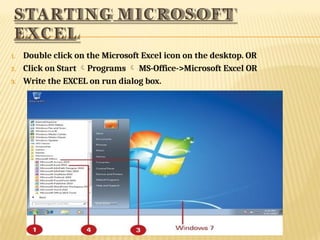
1. Double click on the Microsoft Excel icon on the desktop. OR
2. Click on Start Programs  MS-Office->Microsoft Excel OR
3. Write the EXCEL on run dialog box.
ANATOMY OF MS-EXCEL
When you open MS Excel a window on the screen flashes it has number
of parts.
1 2 3 4 5
6 7 8 9 10
1. THE TITLE BAR :-
Title bar is located at the very top of the screen. On the title
bar, Microsoft excel displays the name of the workbook
you are currently using. At the top of your screen, you
should see
“Microsoft excel-book1” or a similar name.
2. THE MENU BAR :-
The menu bar is directly below the title bar and displays a
list of the menus that you can use to give commands to excel.
Clicking on a menu name displays a drop down menu of
commands. You can move across the menu bar and down the
drop-down menus with your mouse of by highlighting one of the
menu items and using the arrow keys on your keyboard.
 FILE :- file-related commands to open , save ,close ,print
and cerate new files.
 EDIT:- commands to copy, cut, paste, find, and replace
text.
 VIEW:- commands to change how the workbook is
displayed on the screen.
 INSERT:- list items that you can insert into a workbook,
such as graphics and charts.
 FORMAT:- commands to format fonts, cell
alignment, and borders.
 TOOLS:- lists tools such as the spell checker and
macros.
 HELP:- get help on using the excel program
3.THE FORMULA BAR:- If the formula bar is turned on, the cell
address displays on the left side of the formula bar. Cell entries
display on the right side of the formula bar.
4. STANDARD TOOLBAR
🞭 Toolbar is a collection of tools or icons
displayed in a long bar that can move
or reshaped to make it convinent to
use.
🞭 Each icon in a toolbar correspond to
a command
5. FORMATTING TOOLBAR:
🞭 Here various formatting options are
avaliable.
6. Status bar:
 displays the name of the command at the
left hand side of status bar. It gives status
operations in program.
7.WORKSHEET TABS :- You can keep multiple worksheets together in a
group called a workbook. For example you could have a separate
worksheet for each month of the year in a workbook for the year 2010. You
can give worksheets your own meaningful names by placing your cursor
over the sheet name and typing. By default, excel opens with three
worksheets.
HORIZONTAL SCROLLBAR
VERTICAL SCROLLBAR
🞭 Using horizontal and vertical scroll bar you
can move(up or down) and (left or right)
respectively.
ENTERING TEXT
CELLS:- The workbook is made up of cells. There is a cell at the
intersection of each row and column. A cell can contain a value, a formula,
or a text entry. A text entry is used to label or explain the contents or the
value of a formula.
ROWS, COLUMNS AND SHEETS:- The Excel worksheet contains 16,384
rows that extend down the worksheet, numbered 1 through 16384.
The Excel worksheet contains 256 columns that extend across the
worksheet , lettered A through Z, AA through AZ, BA through BZ, and
continuing to IA through IZ.
The Excel worksheet can contain as many as 256 sheets, labeled sheet1
through sheet256.The initial number of sheet in a workbook, which can
be changed by the user is 16.
I N S E R T I N G C E L L S :
WHEN YOU CREATE A WORKSHEET THE NEED TO MOVE THE CELLS
OCCURRED FREQUENTLY. THAT IS INSERTING CELLS, DELETING CELLS.
 INSERTING A COLUMN:
The following are the various steps to insert column in the
worksheet:
1. Select the range of cells in your worksheet.
2. Right click the mouse a shortcut menu appears OR you can also
select cells option from INSERT menu.
3. Select Insert dialog box shortcut menu.
4. Four options appeared.
a) Insert Cell.
b)Insert Sheet Rows
c)Insert Sheet Columns
d)Insert Sheet
5.Selected cells will be free and now you can type the data
onto cells.

INSERTTING A ROW : Inserting rows means inserting row
somewhere in the worksheet. The following are the
steps to insert row:
1. Click the header of a row in your worksheet.
2. Right click the mouse a shortcut menu appears.
3. Select Insert dialog box a new blank row appears
on selected row.
4. When click insert dialog box anew blank row
appears on selected row.
5. You can now type the data in that row.
DELETING CELLS:
DELETING ROW OR COLUMN MEANS YOU WANT TO DELETE ROW OR
COLUMN FROM WORKSHEET.
THE STEPS TO DELETE ROW OR COLUMN ARE SAME AS UNDER:
 DELETING A ROW OR COLUMN:
1. Click the header of a row in your worksheet.
2. Right click the mouse a shortcut menu appears.
3. Select delete dialog box from shortcut menu.
4. Five options appeared:
5. AFTER CLICKING DELETE BOX THE SELECTED ROWS GETS DELETED FROM
WORKSHEET.
 DELETING A CELL ENTRY:
To delete an entry in a cell or a group of cells, you place
the cursor in the
cell or highlight the group of cells and press DELETE.
1. Place the cursor in cell A5.
2. Press the Delete key.
WORKING WITH FORMULAS AND
FUNCTIONS
Entering a Formula:
 A formula is an expression that returns a value.
 A formula is written using operators that combine different
values, returning a single value that is then displayed in the cell.
 The most commonly used operators are arithmetic operators.
 The order of precedence is a set of predefined rules used to
determine the sequence in which operators are applied in a
calculation.
ENTERING A FORMULA:
ENTERING A FORMULA:
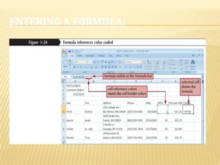
 Click the cell in which you want the formula results to
appear.
 Type = and an expression that calculates a value using
cell references and arithmetic operators.
 Press the Enter key or press the Tab key to complete
the
formula.
ENTERING A FORMULA:
COPYING AND PASTING FORMULAS
 With formulas, however, Excel adjusts the formula’s cell references
to
reflect the new location of the formula in the worksheet
INTRODUCING FUNCTIONS:
 A function is a named operation that returns a value
 For example, to add the values in the range A1:A10, you
could enter the following long formula:
=A1+A2+A3+A4+A5+A6+A7+A8+A9+A10
Or, you could use the SUM function to accomplish
the same thing:
=SUM(A1:A10)
ENTERING A FUNCTION:
ENTERING FUNCTIONS WITH AUTOSUM:
 The AutoSum button quickly inserts Excel functions that summarize
all the values in a column or row using a single statistic
🞤 Sum of the values in the column or row
🞤 Average value in the column or row
🞤 Total count of numeric values in the column or row
🞤 Minimum value in the column or row
🞤 Maximum value in the column or row
ENTERING FUNCTIONS WITH AUTOSUM:
VIEWING AND PRINTING
WORKSHEET FORMULAS
 You can view the formulas in a workbook by switching to formula
view, a view of the workbook contents that displays formulas instead
of the resulting values.
 To change the worksheet to formula view, press the Ctrl+` keys.
 Scaling a printout reduces the width and the height of the printout to
fit the number of pages you specify by shrinking the text size as
needed.
VIEWING AND PRINTING
WORKSHEET FORMULAS:
OBJECTIVES:
 Create an embedded chart
 Work with chart titles and legends
 Create and format a pie chart
 Work with 3D charts
 Create and format a column chart
 Create and format a line chart
 Use custom formatting with chart axes
 Work with tick marks and scale values
 Create and format a combined chart
 Insert and format a graphic shape
 Create a chart sheet
PROTECTING WORKSHEETS/WORKBOOKS
🞭 We need to protect the cells, worksheets,
workbooks from the access of unauthorized
users who may change or copy the data.
🞭 User can apply password to the worksheet in
order to protect it. A password may also be
applied to range of cells.
🞭 Applying password will make worksheet read only.
🞭 When you unprotect it, it will become
read/write file.
CREATING CHARTS:
 A chart, or graph, is a visual representation of a set of data
 Select the data source with the range of data you want to chart
 In the Charts group on the Insert tab, click a chart type, and then click
a chart subtype in the Chart gallery
 In the Location group on the Chart Tools Design tab, click the Move
Chart button to place the chart in a chart sheet or embed it into a
worksheet
CREATING CHARTS:
SELECTING A CHART TYPE:
 Click the Insert tab on the Ribbon
 In the Charts group, click the Pie button
MOVING AND RESIZING CHARTS:
 By default, a chart is inserted as an embedded chart, which means
the chart is placed in a worksheet next to its data source.
 You can also place a chart in a chart sheet.
 In the Location group on the Chart Tools Design tab, click the
Move Chart button.
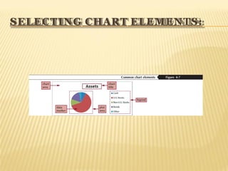
SELECTING CHART ELEMENTS:
CHOOSING A CHART STYLE AND
LAYOUT:
CHOOSING A CHART STYLE AND
LAYOUT:
WORKING WITH THE CHART
TITLE AND LEGEND:
 Click the chart title to select it
 Type the chart title, and then press the Enter key
 Click the Chart Tools Layout tab on the Ribbon
 In the Labels group, click the Legend button, and then click
the desired legend position
WORKING WITH THE CHART
TITLE AND LEGEND:
CREATING A COLUMN CHART:
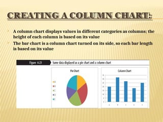
 A column chart displays values in different categories as columns; the
height of each column is based on its value
 The bar chart is a column chart turned on its side, so each bar length
is based on its value
CREATING A COLUMN CHART:
 Select the range.
 Click the Insert tab on the Ribbon.
 In the Charts group, click the Column button and then choose
the chart subtype.
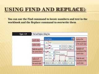
USING FIND AND REPLACE:
 You can use the Find command to locate numbers and text in the
workbook and the Replace command to overwrite them
USING THE SPELLING CHECKER:
 The spelling checker verifies the words in the active worksheet
against the program’s dictionary.
THANKYO
U

Microsoft excel power point presentation.pptx

  • 1.
  • 2.
    INTRODUCTION  Microsoft Excelis allow you to create professional spreadsheets and charts. It is quite useful in entering, editing, analysis and storing of data.  It performs numerous functions and formulas to assist you in your projects.  MS-EXCEL is the replacement of calculator, pencil work. You can create charts with colors, add clip arts in excel .
  • 3.
     A newworkbook contains 256 worksheets. The worksheet is a grid of COLUMNS and ROWS.  The intersection of a column and a row is called a CELL.  Each cell on the spreadsheet has a CELL ADDRESS that is the column letter and the row number.
  • 4.
    FEATURES: 🞭 Data entryusing keyboard 🞭 Worksheet can be saved and retrieved for further editing 🞭 Various formatting options can be used to format the data stored in the cells 🞭 Allows mathematical calculations 🞭 Automatic recalculation is done when previous entries are changed 🞭 Results calculated are reliable 🞭 You can import and export data from one worksheet to another 🞭 The scenario option avaliable helps us to answer “what if” questions
  • 5.
    STARTING M IC R O S O F T E X C E L 1. Double click on the Microsoft Excel icon on the desktop. OR 2. Click on Start Programs  MS-Office->Microsoft Excel OR 3. Write the EXCEL on run dialog box.
  • 6.
    ANATOMY OF MS-EXCEL Whenyou open MS Excel a window on the screen flashes it has number of parts. 1 2 3 4 5 6 7 8 9 10
  • 7.
    1. THE TITLEBAR :- Title bar is located at the very top of the screen. On the title bar, Microsoft excel displays the name of the workbook you are currently using. At the top of your screen, you should see “Microsoft excel-book1” or a similar name. 2. THE MENU BAR :- The menu bar is directly below the title bar and displays a list of the menus that you can use to give commands to excel. Clicking on a menu name displays a drop down menu of commands. You can move across the menu bar and down the drop-down menus with your mouse of by highlighting one of the menu items and using the arrow keys on your keyboard.
  • 8.
     FILE :-file-related commands to open , save ,close ,print and cerate new files.  EDIT:- commands to copy, cut, paste, find, and replace text.  VIEW:- commands to change how the workbook is displayed on the screen.  INSERT:- list items that you can insert into a workbook, such as graphics and charts.  FORMAT:- commands to format fonts, cell alignment, and borders.  TOOLS:- lists tools such as the spell checker and macros.  HELP:- get help on using the excel program
  • 9.
    3.THE FORMULA BAR:-If the formula bar is turned on, the cell address displays on the left side of the formula bar. Cell entries display on the right side of the formula bar.
  • 10.
    4. STANDARD TOOLBAR 🞭Toolbar is a collection of tools or icons displayed in a long bar that can move or reshaped to make it convinent to use. 🞭 Each icon in a toolbar correspond to a command
  • 11.
    5. FORMATTING TOOLBAR: 🞭Here various formatting options are avaliable. 6. Status bar:  displays the name of the command at the left hand side of status bar. It gives status operations in program.
  • 12.
    7.WORKSHEET TABS :-You can keep multiple worksheets together in a group called a workbook. For example you could have a separate worksheet for each month of the year in a workbook for the year 2010. You can give worksheets your own meaningful names by placing your cursor over the sheet name and typing. By default, excel opens with three worksheets.
  • 13.
    HORIZONTAL SCROLLBAR VERTICAL SCROLLBAR 🞭Using horizontal and vertical scroll bar you can move(up or down) and (left or right) respectively.
  • 14.
    ENTERING TEXT CELLS:- Theworkbook is made up of cells. There is a cell at the intersection of each row and column. A cell can contain a value, a formula, or a text entry. A text entry is used to label or explain the contents or the value of a formula. ROWS, COLUMNS AND SHEETS:- The Excel worksheet contains 16,384 rows that extend down the worksheet, numbered 1 through 16384. The Excel worksheet contains 256 columns that extend across the worksheet , lettered A through Z, AA through AZ, BA through BZ, and continuing to IA through IZ. The Excel worksheet can contain as many as 256 sheets, labeled sheet1 through sheet256.The initial number of sheet in a workbook, which can be changed by the user is 16.
  • 15.
    I N SE R T I N G C E L L S : WHEN YOU CREATE A WORKSHEET THE NEED TO MOVE THE CELLS OCCURRED FREQUENTLY. THAT IS INSERTING CELLS, DELETING CELLS.  INSERTING A COLUMN: The following are the various steps to insert column in the worksheet: 1. Select the range of cells in your worksheet. 2. Right click the mouse a shortcut menu appears OR you can also select cells option from INSERT menu.
  • 16.
    3. Select Insertdialog box shortcut menu. 4. Four options appeared. a) Insert Cell. b)Insert Sheet Rows c)Insert Sheet Columns d)Insert Sheet 5.Selected cells will be free and now you can type the data onto cells.
  • 17.
     INSERTTING A ROW: Inserting rows means inserting row somewhere in the worksheet. The following are the steps to insert row: 1. Click the header of a row in your worksheet. 2. Right click the mouse a shortcut menu appears. 3. Select Insert dialog box a new blank row appears on selected row. 4. When click insert dialog box anew blank row appears on selected row. 5. You can now type the data in that row.
  • 18.
    DELETING CELLS: DELETING ROWOR COLUMN MEANS YOU WANT TO DELETE ROW OR COLUMN FROM WORKSHEET. THE STEPS TO DELETE ROW OR COLUMN ARE SAME AS UNDER:  DELETING A ROW OR COLUMN: 1. Click the header of a row in your worksheet. 2. Right click the mouse a shortcut menu appears. 3. Select delete dialog box from shortcut menu. 4. Five options appeared:
  • 19.
    5. AFTER CLICKINGDELETE BOX THE SELECTED ROWS GETS DELETED FROM WORKSHEET.  DELETING A CELL ENTRY: To delete an entry in a cell or a group of cells, you place the cursor in the cell or highlight the group of cells and press DELETE. 1. Place the cursor in cell A5. 2. Press the Delete key.
  • 20.
    WORKING WITH FORMULASAND FUNCTIONS Entering a Formula:  A formula is an expression that returns a value.  A formula is written using operators that combine different values, returning a single value that is then displayed in the cell.  The most commonly used operators are arithmetic operators.  The order of precedence is a set of predefined rules used to determine the sequence in which operators are applied in a calculation.
  • 21.
  • 22.
    ENTERING A FORMULA: Click the cell in which you want the formula results to appear.  Type = and an expression that calculates a value using cell references and arithmetic operators.  Press the Enter key or press the Tab key to complete the formula.
  • 23.
  • 24.
    COPYING AND PASTINGFORMULAS  With formulas, however, Excel adjusts the formula’s cell references to reflect the new location of the formula in the worksheet
  • 25.
    INTRODUCING FUNCTIONS:  Afunction is a named operation that returns a value  For example, to add the values in the range A1:A10, you could enter the following long formula: =A1+A2+A3+A4+A5+A6+A7+A8+A9+A10 Or, you could use the SUM function to accomplish the same thing: =SUM(A1:A10)
  • 26.
  • 27.
    ENTERING FUNCTIONS WITHAUTOSUM:  The AutoSum button quickly inserts Excel functions that summarize all the values in a column or row using a single statistic 🞤 Sum of the values in the column or row 🞤 Average value in the column or row 🞤 Total count of numeric values in the column or row 🞤 Minimum value in the column or row 🞤 Maximum value in the column or row
  • 28.
  • 29.
    VIEWING AND PRINTING WORKSHEETFORMULAS  You can view the formulas in a workbook by switching to formula view, a view of the workbook contents that displays formulas instead of the resulting values.  To change the worksheet to formula view, press the Ctrl+` keys.  Scaling a printout reduces the width and the height of the printout to fit the number of pages you specify by shrinking the text size as needed.
  • 30.
  • 31.
    OBJECTIVES:  Create anembedded chart  Work with chart titles and legends  Create and format a pie chart  Work with 3D charts  Create and format a column chart  Create and format a line chart  Use custom formatting with chart axes  Work with tick marks and scale values  Create and format a combined chart  Insert and format a graphic shape  Create a chart sheet
  • 32.
    PROTECTING WORKSHEETS/WORKBOOKS 🞭 Weneed to protect the cells, worksheets, workbooks from the access of unauthorized users who may change or copy the data. 🞭 User can apply password to the worksheet in order to protect it. A password may also be applied to range of cells. 🞭 Applying password will make worksheet read only. 🞭 When you unprotect it, it will become read/write file.
  • 33.
    CREATING CHARTS:  Achart, or graph, is a visual representation of a set of data  Select the data source with the range of data you want to chart  In the Charts group on the Insert tab, click a chart type, and then click a chart subtype in the Chart gallery  In the Location group on the Chart Tools Design tab, click the Move Chart button to place the chart in a chart sheet or embed it into a worksheet
  • 34.
  • 35.
    SELECTING A CHARTTYPE:  Click the Insert tab on the Ribbon  In the Charts group, click the Pie button
  • 36.
    MOVING AND RESIZINGCHARTS:  By default, a chart is inserted as an embedded chart, which means the chart is placed in a worksheet next to its data source.  You can also place a chart in a chart sheet.  In the Location group on the Chart Tools Design tab, click the Move Chart button.
  • 37.
  • 38.
    CHOOSING A CHARTSTYLE AND LAYOUT:
  • 39.
    CHOOSING A CHARTSTYLE AND LAYOUT:
  • 40.
    WORKING WITH THECHART TITLE AND LEGEND:  Click the chart title to select it  Type the chart title, and then press the Enter key  Click the Chart Tools Layout tab on the Ribbon  In the Labels group, click the Legend button, and then click the desired legend position
  • 41.
    WORKING WITH THECHART TITLE AND LEGEND:
  • 42.
    CREATING A COLUMNCHART:  A column chart displays values in different categories as columns; the height of each column is based on its value  The bar chart is a column chart turned on its side, so each bar length is based on its value
  • 43.
    CREATING A COLUMNCHART:  Select the range.  Click the Insert tab on the Ribbon.  In the Charts group, click the Column button and then choose the chart subtype.
  • 44.
    USING FIND ANDREPLACE:  You can use the Find command to locate numbers and text in the workbook and the Replace command to overwrite them
  • 45.
    USING THE SPELLINGCHECKER:  The spelling checker verifies the words in the active worksheet against the program’s dictionary.
  • 46.