Sir Kashif
Lecture 3:
Introduction to Excel
Objectives
Definition and functions of spreadsheets
 Basic components of Excel
 Creating workbooks and worksheets
 Navigation
 Data entry
 Formatting (data and cells)
 Creating simple formulas
 Printing
 Creating graphs and charts
Definition and Functions
 An electronic ledger developed to
ease time-consuming numeric
calculations like budgets, grades,
etc.
 Functions as a simple database,
allowing easy manipulation of
data to include search and sort,
etc.
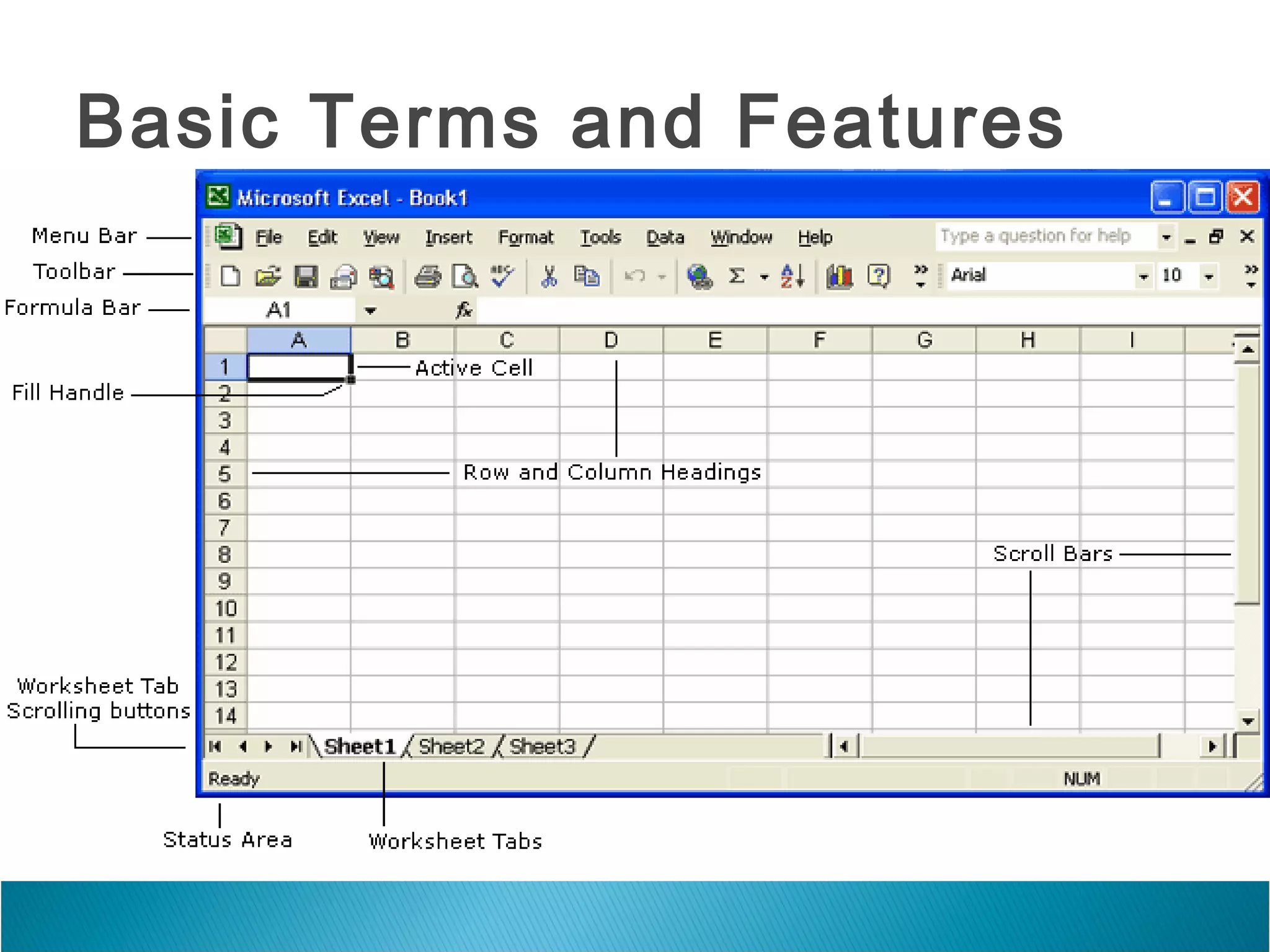
Basic Terms and Features
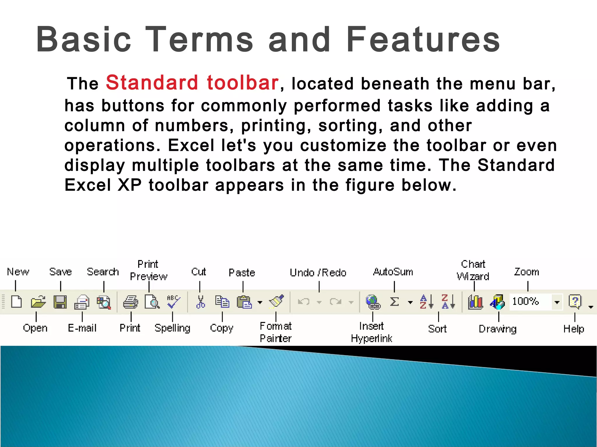
The Standard toolbar, located beneath the menu bar,
has buttons for commonly performed tasks like adding a
column of numbers, printing, sorting, and other
operations. Excel let's you customize the toolbar or even
display multiple toolbars at the same time. The Standard
Excel XP toolbar appears in the figure below.
The Formatting toolbar, located beneath
the Standard toolbar bar, has buttons for
various formatting operations like
changing text size or style, formatting
numbers and placing borders around cells.
Basic Terms and Features
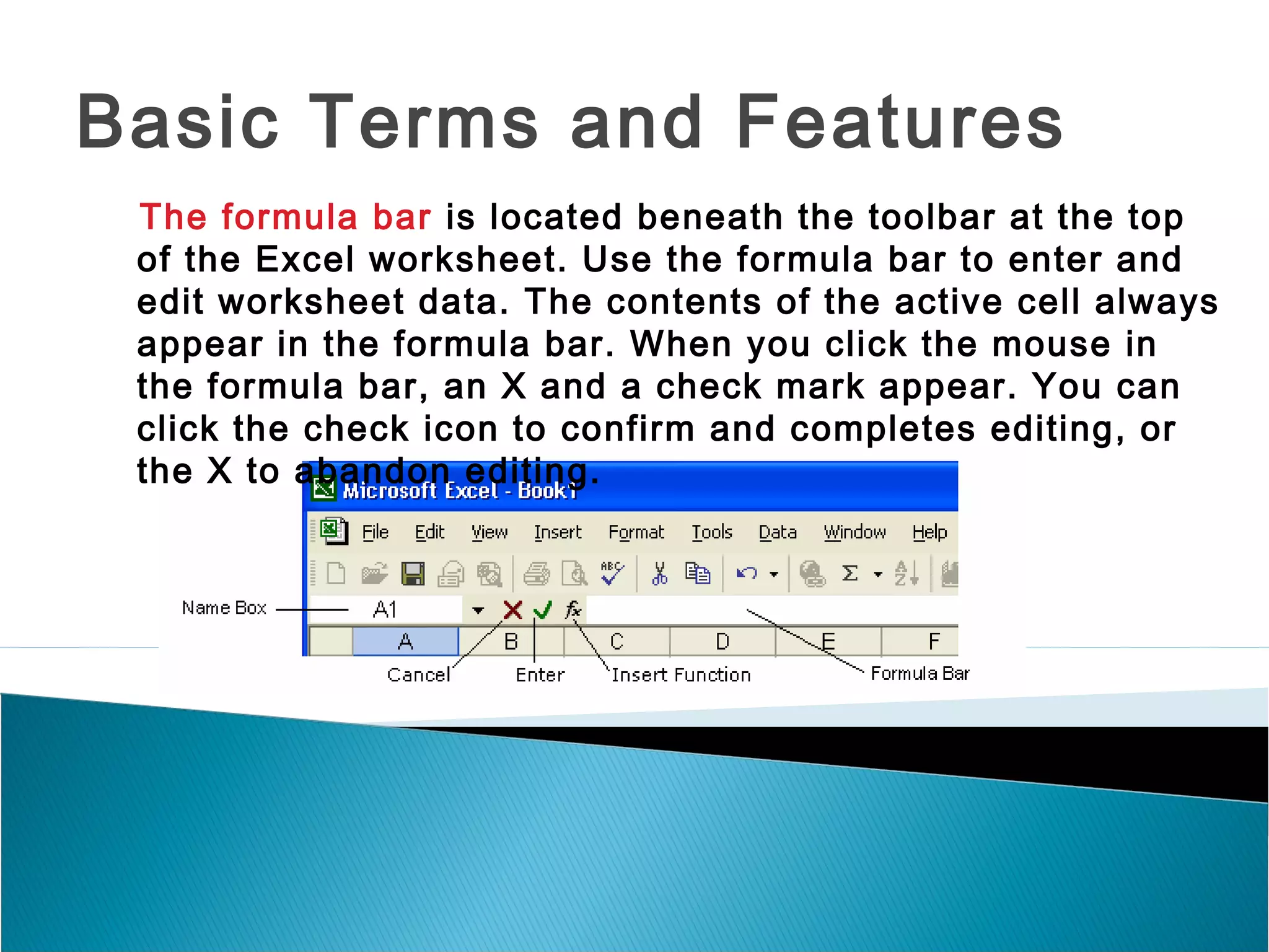
The formula bar is located beneath the toolbar at the top
of the Excel worksheet. Use the formula bar to enter and
edit worksheet data. The contents of the active cell always
appear in the formula bar. When you click the mouse in
the formula bar, an X and a check mark appear. You can
click the check icon to confirm and completes editing, or
the X to abandon editing.
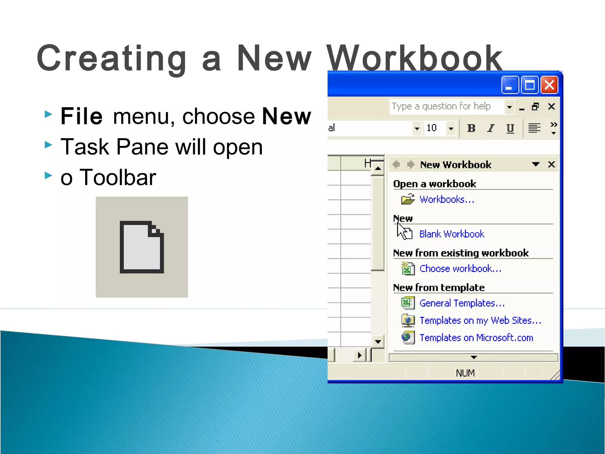
Creating a New Workbook
 File menu, choose New
 Task Pane will open
 o Toolbar
Creating/Adding a Worksheet
 Select Insert, then Worksheet
 Go to a worksheet tab, right click on your mouse,
choose Insert, if worksheet icon is highlighted in
blue, hit OK
Naming/Renaming a
Worksheet
 Move curser to the worksheet tab you want to name
 Right click on your mouse
 Choose Rename
 The worksheet tab will be highlighted
 Hit the delete key to erase current name
 Type in the new name for the worksheet
 Select File, Save, or Save As or use toolbar icon to
save changes
 Go to File, then Save, or toolbar icon of a
diskette
 Delete highlighted name in the File
 Name: box
 Type in desired file name and click Save to
complete the save procedure
Naming a New Worksheet
Navigation
 Refer to the table below for additional
information on using the keyboard to
navigate a worksheet.
To move Press this key
One cell left Left Arrow
One cell right Right Arrow
One cell up Up Arrow
One cell down Down Arrow
To top of worksheet (cell A1) Control Home
To last cell containing data Control End
To end of data in a column Control Down Arrow
To beginning of data in a
column
Control Up Arrow
To end of data in a row Control Right Arrow
To beginning of data in a row Control Left Arrow
Data Entry
Entering Data
 Label (text)
 Values (numbers and dates)
Editing Data
 Select the cell and retype entry (works well with numbers)
 Use the formula bar (works well with text)
Clearing Cell Contents
 Choose Clear from the Edit menu
 Press the Delete key
Undoing Mistakes
 Use the Undo command on the Edit menu
 Use the Undo tool to correct the mistake
Copy Data
 Copy selected data from one cell to another with the Copy and Paste
commands
 Use the Drag and Drop procedure
Move Data
 Use the Cut and Paste commands
 Use the Drag and Drop procedure
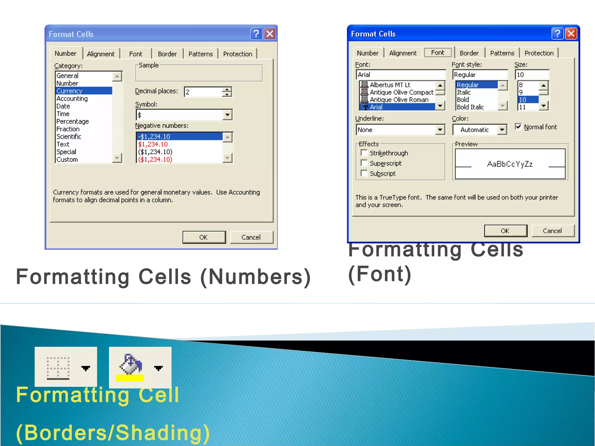
Formatting Cells
(Font)
Formatting Cells (Numbers)
Formatting Cell
(Borders/Shading)
Building a Formula Formula
(AutoSum)
-Select the cell in which
you want the results to
appear
-Go to Insert Function
-The AutoSum screen
will appear
-Move the highlighted
bar to the desired
function (Sum, If,
Average, etc.) or
category
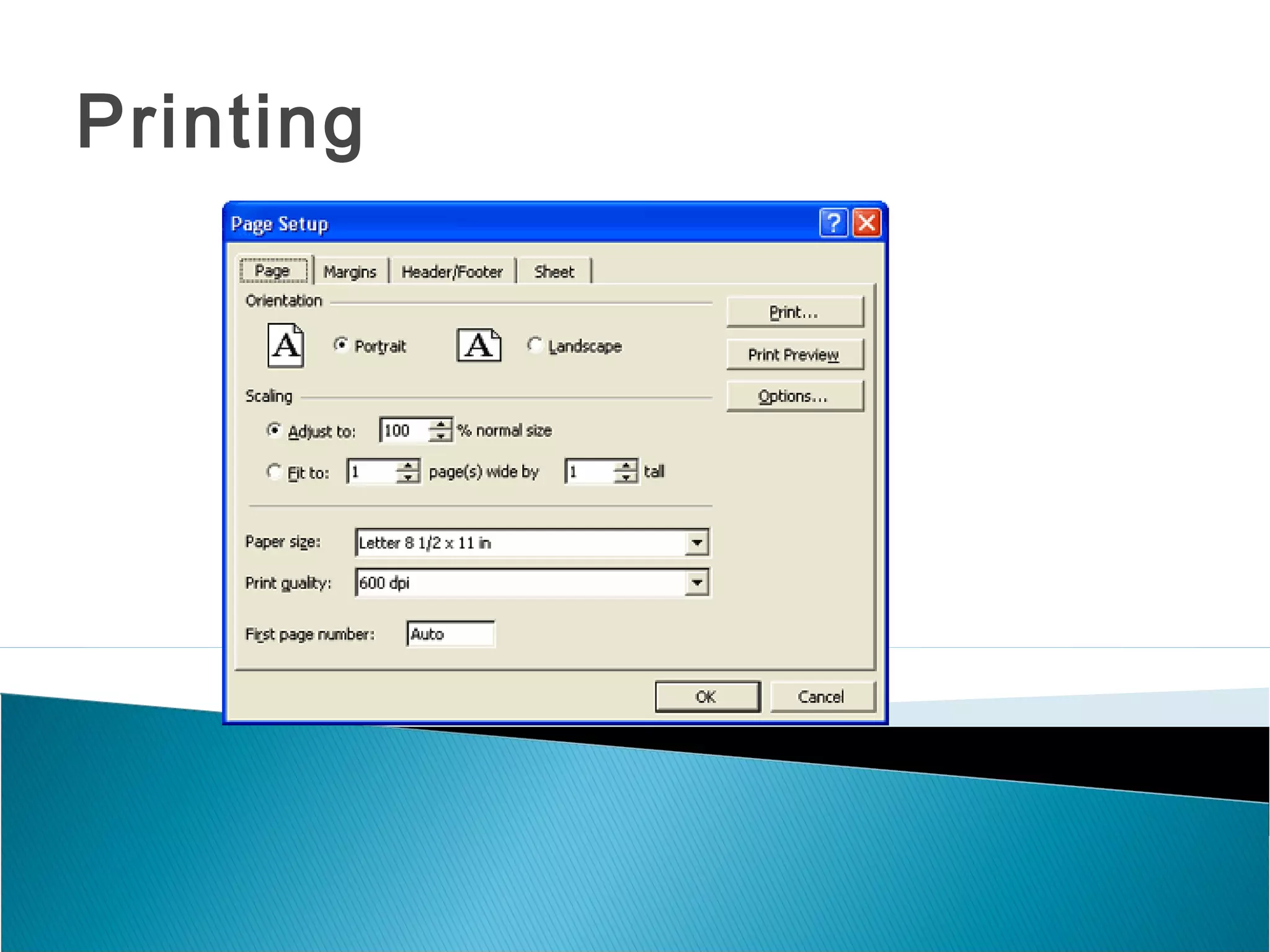
Printing
Chart
 To create a chart in Microsoft Excel,
select the data you wish to graph
and choose Chart… from the
Insert menu, or click
 on the Chart Wizard () button on
the standard toolbar.
Step 1
 Select Standard or Custom
Chart Type;
 select Chart sub-type
 The Press and hold to view
sample button will show you a tiny
preview of your data's chart
Chart
Step 2
 Step two allows you to choose the Chart's
Source
 Data. This is the data you want to graph.
Here we
 can also see a sample of the chart. If
Excel is
 charting the wrong data, simply click on
the
 collapse button ("go out and get it"
button) () and
 choose the data you wish to graph, once it
is
 selected, press enter to return to this
window.
 From this Data Range tab you can also
change the Series in: option, such that
instead of charting the data by column, it
will chart the data by row.
Chart
Step 3
 Each part of the Chart can be changed with in the options.
After the chart is created you will still be able to change these
options
 The Chart title: goes across the top of the graph, the
Category (X) axis: goes under our
 X-axis labels (shown here as Pants, Shoes, Socks…), the
Value (Y) axis: will be the label
 for the vertical labels (shown here as 2500,
 2000, 1500…)
 These titles will not show up on your sample chart until you
have left that text box. (Click somewhere else in the window)
Chart
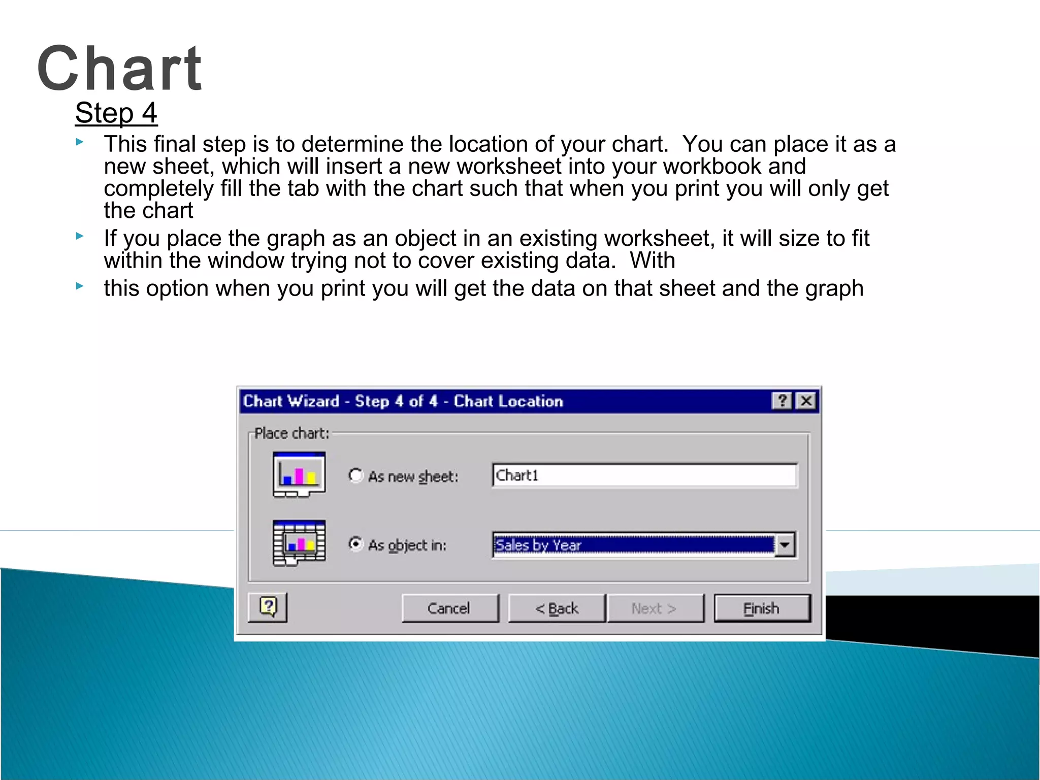
Step 4
 This final step is to determine the location of your chart. You can place it as a
new sheet, which will insert a new worksheet into your workbook and
completely fill the tab with the chart such that when you print you will only get
the chart
 If you place the graph as an object in an existing worksheet, it will size to fit
within the window trying not to cover existing data. With
 this option when you print you will get the data on that sheet and the graph

excell.pdf

  • 1.
  • 2.
    Objectives Definition and functionsof spreadsheets  Basic components of Excel  Creating workbooks and worksheets  Navigation  Data entry  Formatting (data and cells)  Creating simple formulas  Printing  Creating graphs and charts
  • 3.
    Definition and Functions An electronic ledger developed to ease time-consuming numeric calculations like budgets, grades, etc.  Functions as a simple database, allowing easy manipulation of data to include search and sort, etc.
  • 4.
  • 5.
    Basic Terms andFeatures The Standard toolbar, located beneath the menu bar, has buttons for commonly performed tasks like adding a column of numbers, printing, sorting, and other operations. Excel let's you customize the toolbar or even display multiple toolbars at the same time. The Standard Excel XP toolbar appears in the figure below.
  • 6.
    The Formatting toolbar,located beneath the Standard toolbar bar, has buttons for various formatting operations like changing text size or style, formatting numbers and placing borders around cells. Basic Terms and Features
  • 7.
    Basic Terms andFeatures The formula bar is located beneath the toolbar at the top of the Excel worksheet. Use the formula bar to enter and edit worksheet data. The contents of the active cell always appear in the formula bar. When you click the mouse in the formula bar, an X and a check mark appear. You can click the check icon to confirm and completes editing, or the X to abandon editing.
  • 8.
    Creating a NewWorkbook  File menu, choose New  Task Pane will open  o Toolbar
  • 9.
    Creating/Adding a Worksheet Select Insert, then Worksheet  Go to a worksheet tab, right click on your mouse, choose Insert, if worksheet icon is highlighted in blue, hit OK
  • 10.
    Naming/Renaming a Worksheet  Movecurser to the worksheet tab you want to name  Right click on your mouse  Choose Rename  The worksheet tab will be highlighted  Hit the delete key to erase current name  Type in the new name for the worksheet  Select File, Save, or Save As or use toolbar icon to save changes
  • 11.
     Go toFile, then Save, or toolbar icon of a diskette  Delete highlighted name in the File  Name: box  Type in desired file name and click Save to complete the save procedure Naming a New Worksheet
  • 12.
    Navigation  Refer tothe table below for additional information on using the keyboard to navigate a worksheet. To move Press this key One cell left Left Arrow One cell right Right Arrow One cell up Up Arrow One cell down Down Arrow To top of worksheet (cell A1) Control Home To last cell containing data Control End To end of data in a column Control Down Arrow To beginning of data in a column Control Up Arrow To end of data in a row Control Right Arrow To beginning of data in a row Control Left Arrow
  • 13.
    Data Entry Entering Data Label (text)  Values (numbers and dates) Editing Data  Select the cell and retype entry (works well with numbers)  Use the formula bar (works well with text) Clearing Cell Contents  Choose Clear from the Edit menu  Press the Delete key Undoing Mistakes  Use the Undo command on the Edit menu  Use the Undo tool to correct the mistake Copy Data  Copy selected data from one cell to another with the Copy and Paste commands  Use the Drag and Drop procedure Move Data  Use the Cut and Paste commands  Use the Drag and Drop procedure
  • 14.
    Formatting Cells (Font) Formatting Cells(Numbers) Formatting Cell (Borders/Shading)
  • 15.
    Building a FormulaFormula (AutoSum) -Select the cell in which you want the results to appear -Go to Insert Function -The AutoSum screen will appear -Move the highlighted bar to the desired function (Sum, If, Average, etc.) or category
  • 16.
  • 17.
    Chart  To createa chart in Microsoft Excel, select the data you wish to graph and choose Chart… from the Insert menu, or click  on the Chart Wizard () button on the standard toolbar. Step 1  Select Standard or Custom Chart Type;  select Chart sub-type  The Press and hold to view sample button will show you a tiny preview of your data's chart
  • 18.
    Chart Step 2  Steptwo allows you to choose the Chart's Source  Data. This is the data you want to graph. Here we  can also see a sample of the chart. If Excel is  charting the wrong data, simply click on the  collapse button ("go out and get it" button) () and  choose the data you wish to graph, once it is  selected, press enter to return to this window.  From this Data Range tab you can also change the Series in: option, such that instead of charting the data by column, it will chart the data by row.
  • 19.
    Chart Step 3  Eachpart of the Chart can be changed with in the options. After the chart is created you will still be able to change these options  The Chart title: goes across the top of the graph, the Category (X) axis: goes under our  X-axis labels (shown here as Pants, Shoes, Socks…), the Value (Y) axis: will be the label  for the vertical labels (shown here as 2500,  2000, 1500…)  These titles will not show up on your sample chart until you have left that text box. (Click somewhere else in the window)
  • 20.
    Chart Step 4  Thisfinal step is to determine the location of your chart. You can place it as a new sheet, which will insert a new worksheet into your workbook and completely fill the tab with the chart such that when you print you will only get the chart  If you place the graph as an object in an existing worksheet, it will size to fit within the window trying not to cover existing data. With  this option when you print you will get the data on that sheet and the graph