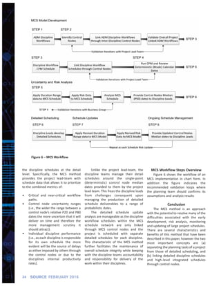
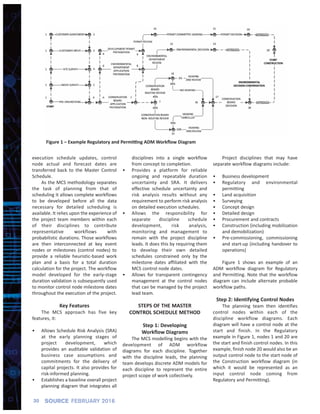
The document proposes a new Master Control Schedule (MCS) Planning and Risk Analysis method to address challenges with traditional schedule risk analysis (SRA) and project scheduling. The key aspects of the new method are: 1) It separates planning from detailed scheduling, allowing planning and risk analysis to occur earlier before detailed schedules exist. 2) It uses a workflow-based Arrow Diagramming Method (ADM) master control schedule integrated with discrete execution schedules through control nodes. 3) It allows for schedule risk analysis, planning, contingency management and updates to all occur within an integrated process linked to the master control schedule.

1. 28 SOURCE FEBRUARY 2016
Master Control Schedule –
Planning and Risk Analysis Method
Yaroslav Kovalenko, Martin J. Gough, P.Eng.,
and Dr. Mark Krahn
I
nexpensive, fast and increasingly
more sophisticated Monte Carlo
simulation software packages
have become a catalyst for more
elaborate approaches to Schedule Risk
Analysis (SRA). Over the past 10 years or
so, there have been increasing numbers
of journal articles published on the
subject of SRAs and in the authors’
experience, project teams are adopting
CPM‐based SRAs ever more readily.
Despite the enhanced focus on SRAs,
many practitioners and project team
members will attest to the challenges
associated with conducting meaningful
SRAs. The fundamental nature of SRA
and its absolute dependency on the
integrity of the schedule being assessed
creates unique challenges in properly
modeling the inputs and correctly
interpreting the outputs, especially in
the early stages of projects.
A recent article effectively
summarizes the goal of the Master
Control Schedule (MCS) Planning and
Risk Analysis method presented herein.
Sriram Ramdass, PSP, and Jihwan Lim,
PSP, succinctly note that “…a more
sustainable and simple approach to
schedule risk analysis where the level of
effort and sophistication of the risk
analysis process is tailored to fit the
project need, has the potential to add
value and improve schedule
performance” [1].
While it is well recognized that
scheduling is a key skill that plays a
critical role in any project organization, it
is the authors’ experience that schedule
management, including SRA, is still
immature in many organizations. To
elaborate on this generic criticism of
project schedule management and SRA
and to provide a fundamental basis for
understanding the methodology, a
review of current pertinent literature
follows.
There are four key themes in the
literature related to schedule
management and SRA that provide
context for the proposed methodology.
Those themes are: schedule risk
analysis, schedule planning, schedule
contingency, and schedule updates.
Each theme is elaborated as follows.
Schedule Risk Analysis (SRA)
The majority of the SRA literature is
focused on steps, tips, and checklists in
order to conduct successful SRAs [2a,
2b, 2c, 2d, 2e]. While these are good
considerations and arguably best
practices for a single SRA or specific
project assessment, there is a
fundamental lack of integrated process
that can be easily repeated, built‐upon,
and tailored to fit the project needs.
Abstract: The requirement to provide schedule risk assessment at early stages
of project development, when no detailed schedules have been developed, has
proven to be problematic. Then again, this is also true throughout project exe‐
cution as detailed schedules are developed, elaborated, and revised. The require‐
ment of risk assessment to deliver transparent and consistent outcome forecasts
is frequently in conflict with the equal requirement of execution schedules to di‐
rect and monitor day‐to‐day progress of the work.
The authors propose that the solution to this intractable problem lies in rec‐
ognizing that planning and scheduling are discrete functions, each suited to its
own application and each requiring its own skill set. The Master Control Schedule
(MCS) Planning and Risk Analysis method described in this article comprises a
process that separates the planning process from that of detailed scheduling.
This resolves those difficulties associated with the early development, risk analy‐
sis, monitoring, and updating of large project schedules. This article was first
presented as PS.2046 at the 2015 AACE International Annual Meeting in Las
Vegas.
• BONUS CONTENT - TECHNICAL ARTICLE •

2. SRAs are most often viewed as a
separate, stand‐alone activity, and there
is often no link through project controls
to schedule management. Each SRA
requires significant efforts to build (and
re‐build) a schedule model that is
suitable for SRA purposes and then
conduct the analysis. Once the SRA is
complete and the outputs are
determined, it is often set aside with no
further relevance to the master project
schedule, or to overall project
management. If the SRA could be
integrated with the master schedule, it is
probable that not only would the full
value of SRA be realized but the risk
culture of the organization would
improve as well.
Schedule Planning
Although risk management, as
described by both AACE® International
and the Project Management Institute®
(PMI®), project management
frameworks is largely considered a
planning exercise, it seems incongruous
that virtually every article published on
SRA methodology requires a schedule to
be completed (or at least largely
completed) prior to analysis. AACE
International Recommended Practice
61R‐10, Schedule Design – As Applied in
Engineering, Procurement and
Construction is a good checklist for
planning a project and developing a
schedule, however there is no focus on
risk whatsoever in the process [3]. The
authors believe that risk‐informed
planning is a novel approach that leads
to higher integrity CPM schedules.
Therefore, one of the key facets of the
proposed methodology is SRA as a tool
to develop the initial project schedule.
Schedule Contingency
There are informative articles
describing schedule contingency,
however there is no clear consensus on
how to manage it [4a, 4b]. As noted
previously, typically SRA is not linked to a
process whereby the SRA‐determined
schedule contingency informs the
master schedule through tie‐points or
nodes. This can create controversy and
confusion about what to do with the
contingency. The methodology
described in this article includes a
transparent contingency management
strategy at key milestones.
Schedule Updates
A recent article described the “zero‐
step schedule” and in the process the
significant effort and skill required to
maintain the integrity of complex,
multiple‐activity CPM schedules through
update cycles [5]. It seems almost always
the case that schedule integrity
diminishes throughout the update cycles
on most large‐scale projects, assuming
the notion that integrity existed in the
original schedule. As any schedule
analyst will attest, through each update
the number of missing relationship links
and constrained dates often increases,
eventually reducing the schedule to an
elaborate Gantt chart. The authors
believe that this can be attributed to a
lack of application of thorough schedule
update processes; caused by a lack of
execution, or perhaps patience, of the
project team.
An Intractable Problem
The requirement to provide SRAs at
early stages of project development,
when no detailed schedules have been
developed, has proven to be
problematic. Then throughout project
execution, as detailed schedule are
developed, elaborated, and revised, SRA
has proven to be equally challenging.
The requirement of risk assessment to
deliver transparent and consistent
outcome forecasts is frequently in
conflict with the equal requirement of
execution schedules to direct and
monitor day‐to‐day progress of the
work.
A Proposed Solution
This article will address these issues
by discussing a proposed methodology
that recognizes that planning and
scheduling are not simply increasing
levels of elaboration of the same
process, but discrete functions; each
suited to its own application and each
requiring its own skill set. The Master
Control Schedule (MCS) Planning and
Risk Analysis method described herein
comprises a process that by separating
the planning process from that of
detailed scheduling resolves those
difficulties associated with the early
development, risk analysis, monitoring,
and updating of large project schedules.
In the Master Control Schedule
(MCS) method, risk analysis, schedule
planning, schedule contingency
management and schedule updates all
take place within an integrated
workflow‐planning model of the overall
project. The detailed scheduling
required to resource load, manage work
timelines, and monitor productivity
consist of separate exercises connected
to the MCS through counterpart control
node milestones.
This article describes the MCS
approach and features. The eight steps
of an MCS implementation from
developing the initial Arrow
Diagramming Method (ADM) workflows,
through SRA to ongoing schedule
management are described with
illustrative examples.
MASTER CONTROL
SCHEDULE PLANNING AND
RISK ANALYSIS METHOD
Master Control Scheduling
(MCS) Approach
The MCS methodology integrates a
workflow‐based Arrow Diagramming
Method (ADM) Master Control Schedule
with execution schedules through
control nodes. Workflow modeling uses
the Arrow Diagramming Method (ADM)
also referred to as Activity‐on‐Arrow
(AOA). ADM diagrams differ from
Precedence Diagrams (PDM) in that their
graphics represent workflow and critical
work paths with only finish‐to‐start
relationships. Once the ADM is complete
and validated by the project lead‐team it
is modeled in a PDM CPM application to
perform schedule analysis, ideally
retaining only the finish‐to‐start
relationships characteristic of ADM.
Control nodes are defined as those
event points or milestones that
otherwise discrete discipline or area
schedules have in common. Once all of
the control nodes are identified they are
modelled in a control level CPM network
(the Master Control Schedule) suitable
for stochastic analysis. Because the
control nodes are dependency‐linked to
key milestone events in the discipline
schedules, contingency can be
transferred directly to the execution
schedules. Subsequently throughout
29SOURCE FEBRUARY 2016

3. execution schedule updates, control
node actual and forecast dates are
transferred back to the Master Control
Schedule.
As the MCS methodology separates
the task of planning from that of
scheduling it allows complete workflows
to be developed before all the data
necessary for detailed scheduling is
available. It relies upon the experience of
the project team members within each
of their disciplines to contribute
representative workflows with
probabilistic durations. Those workflows
are then interconnected at key event
nodes or milestones (control nodes) to
provide a reliable heuristic‐based work
plan and a basis for a total duration
calculation for the project. The workflow
model developed for the early‐stage
duration validation is subsequently used
to monitor control node milestone dates
throughout the execution of the project.
Key Features
The MCS approach has five key
features, it:
• Allows Schedule Risk Analysis (SRA)
at the early planning stages of
project development, which
provides an auditable validation of
business case assumptions and
commitments for the delivery of
capital projects. It also provides for
risk‐informed planning.
• Establishes a baseline overall project
planning diagram that integrates all
disciplines into a single workflow
from concept to completion.
• Provides a platform for reliable
ongoing and repeatable duration
uncertainty and SRA. It delivers
effective schedule uncertainty and
risk analysis results without any
requirement to perform risk analysis
on detailed execution schedules.
• Allows the responsibility for
separate discipline schedule
development, risk analysis,
monitoring and management to
remain with the project discipline
leads. It does this by requiring them
to develop their own detailed
schedules constrained only by the
milestone dates affiliated with the
MCS control node dates.
• Allows for transparent contingency
management at the control nodes
that can be managed by the project
lead team.
STEPS OF THE MASTER
CONTROL SCHEDULE METHOD
Step 1: Developing
Workflow Diagrams
The MCS modelling begins with the
development of ADM workflow
diagrams for each discipline. Together
with the discipline leads, the planning
team develops discrete ADM models for
each discipline to represent the entire
project scope of work collectively.
Project disciplines that may have
separate workflow diagrams include:
• Business development
• Regulatory and environmental
permitting
• Land acquisition
• Surveying
• Concept design
• Detailed design
• Procurement and contracts
• Construction (including mobilization
and demobilization)
• Pre‐commissioning, commissioning
and start‐up (including handover to
operations)
Figure 1 shows an example of an
ADM workflow diagram for Regulatory
and Permitting. Note that the workflow
diagram can include alternate probable
workflow paths.
Step 2: Identifying Control Nodes
The planning team then identifies
control nodes within each of the
discipline workflow diagrams. Each
diagram will have a control node at the
start and finish. In the Regulatory
example in Figure 1, nodes 1 and 20 are
the start and finish control nodes. In this
example, finish node 20 would also be an
output control node to the start node of
the Construction workflow diagram (in
which it would be represented as an
input control node coming from
Regulatory and Permitting).
30 SOURCE FEBRUARY 2016
Figure 1 – Example Regulatory and Permitting ADM Workflow Diagram

4. Control nodes can be linked
between different discipline start and
finish nodes or at various points in‐
between. For example, Figure 2 shows
the control node at “Design Complete to
60 Percent” of the Detail Engineering
Design discipline workflow
interconnected to the start node of the
“Material Purchase Request for
Quotation (RFQ)” activity of the
Procurement and Contracts workflow.
A separate workflow sheet, the
Control Nodes Worksheet, will show all
of the start, finish, and interconnecting
control nodes. The individual discipline
workflow diagrams along with the
control node worksheet forms a
complete workflow model for the overall
project.
Step 3: Building the
Master Control Schedule
Once all of the discrete discipline
workflows have been completed and
reviewed with both the discipline leads
and the project lead‐team, the logic is
used to develop CPM schedules for each
discipline. Each schedule then becomes
a sub‐schedule for the overall Master
Control Schedule. The Master Control
Schedule consists of sub‐schedules for
each of the disciplines linked through
control nodes. The control nodes
schedule will consist only of milestones.
One milestone dependency is connected
to the start and one to the finish of each
discipline sub‐schedule (nodes 1 and 20
in the example in Figure 1). Additional
milestones are connected at each
intermediate control node dependency
(see Engineering Design node 23 and
Procurement and Contracts node 15 in
the example in Figure 2).
A key feature of the MCS method is
that it links all discipline start, finish and
inter‐discipline control nodes through
the control node sub‐schedule. As a
consequence the project lead‐team can
focus on managing the key events in the
overall schedule. The discipline teams
then each remain separately
accountable and responsible for delivery
of their own sub‐project within the
schedule constraints of the project
control node dates. During execution the
schedule reporting responsibility of the
discipline leads is to provide timely
information about any changes to the
forecast milestone dates for control
node milestones within their discipline
work scope.
Figure 3 shows the relationship
between Engineering Design control
node 23 and Procurement and
Contracting control node 15 within the
MCS. It also highlights the level of
schedule detail within the MCS at both
the control node level and the discipline
level.
Step 4: Applying Durations
to the Master Control Schedule
Once the MCS schedule network is
complete the discipline teams will
estimate durations for each activity in
their ADM workflow diagram. Applying
these durations to each discipline sub‐
schedule will provide a first iteration of a
deterministic duration for the overall
project. Likely, it will be the case that the
schedule network will be subject to
additional logic and duration data
reviews and analysis. This will be
necessary to maintain alignment both
between the separate disciplines and
with any calendar requirements of the
business case.
Step 5: Performing Uncertainty
and Schedule Risk Analysis
of the Master Control Schedule
Once there is alignment between
the disciplines and the business case
based on workflow and likely durations,
uncertainty and risk analysis of the MCS
schedule network can proceed. Low (or
best‐case) and high (or worse‐case)
duration data points are solicited from
the discipline teams around the likely
(mode) activity durations provided in
Step 4. Risk workshops are then
conducted with the full project team to
identify additional event risks with
duration impacts for the MCS schedule
network activities followed by risk
evaluation and mitigation by the project
lead‐team.
The duration ranges and activity
schedule event risks in the MCS are
analyzed using stochastic methods to
assess probable dates for both overall
31SOURCE FEBRUARY 2016
Figure 2 – Example of Interconnecting Control Nodes

5. project completion and for the control
nodes. The overall project completion
probability is then reviewed with the
business team. Typically, the business
team will establish as a target a
calculated completion date with a
probability of 70 to 90 percent. This
target will be a consequence of the level
of business risk tolerance for a project
duration overrun of the committed
completion time.
Step 6: Building Detailed
Execution Schedules
Typically, not all disciplines will
produce their detailed schedules at the
same time. Rather the detailed
schedules will be developed first for the
early disciplines, such as Regulatory and
Environmental Permitting and concept
design. To provide an overall
uncertainty‐based forecast for the
project, the MCS method only needs to
accommodate detailed schedules as
they can reasonably be developed or as
they become available.
The discipline leads will be provided
with calendar date probability results for
each of their discipline control nodes.
They will be required to develop their
own separate detailed discipline
schedules (see Figure 4). Those detailed
schedules will be required to identify as
milestones the detailed schedule
32 SOURCE FEBRUARY 2016
Figure 3 – Example of MCS CPM Model for Detail Engineering and Procurement Disciplines
Figure 4 – Distribution of Table of Probable Calendar Dates

6. 33SOURCE FEBRUARY 2016
counterparts of the MCS control nodes.
In addition, the detailed schedule CPM
analysis will be required to return
milestone dates for the MCS control
node counterparts equal to the median
(P50) date from the MCS analysis.
The MCS method does not require
that an overall detailed schedule is
developed and maintained for the entire
project. Overall project schedule
consequences of execution stage
changes within the discipline detailed
schedules are reported and analysed by
transferring the revised discipline control
node forecast calendar dates back into
the MCS schedule network as likely
(mode) dates. As shown in Figure 4, the
MCS method facilities schedule
uncertainty and risk assessment both
initially and throughout execution
without the requirement to perform SRA
on detailed execution schedules.
Step 7: Performing
Regular Schedule Updates
At the prescribed schedule risk
review intervals, the low and high
durations around the revised mode
durations are collected in risk workshops
along with contemporary activity event
risk information. Once this data is
collected the MCS schedule network is
re‐analysed and new control node
median data dates are returned to the
discipline leads for them to revise their
schedules, if required.
It may be the case that in the
interval between the prescribed
schedule risk reviews there have been
consequential changes to the overall
workflow logic. For example, the
business group may require an
acceleration of the completion date. To
accommodate this the project lead‐team
took the tactical decision to issue the
material purchase RFQ at 30 percent
engineering. The overall schedule would
then be shortened, although at the risk
of issuing an incomplete bill of
quantities. In this case, the logic link to
control node 23 of Engineering in Figure
3 would be replaced in the MCS schedule
network by a logic link to the node at the
completion of 30 percent Engineering
(node 22). Engineering Design node 23
would no longer be a control node and
would be replaced in the control nodes
schedule by new control node 22 (Figure
5). In addition, the risk‐consequence of
issuing an RFQ with an incomplete bill of
quantities would have to be assessed for
all activities upon which it could have a
duration impact.
Regular schedule update sub‐steps
are as follows:
1. The discipline teams advise of any
changes to their discipline ADM
workflow.
2. The discipline teams collect and
report actual and forecast control
node dates to the risk assessment
team.
3. The risk assessment team updates
the MCS schedule network logic
consequent to any changes in the
discipline ADM workflows and
affected control node
dependencies.
4. The risk assessment team collects
and reconciles the control node data
and then performs the MCS
schedule network stochastic
analysis with the current duration
range and activity event risk data
provided by the discipline teams.
5. The risk assessment team returns
the updated control node median
dates to the discipline teams for
them to affect their detail schedule
revisions to remain consistent with
the revised MCS schedule network.
Step 8: Ongoing
Schedule Management
In the MCS method, schedule
contingency is identified as the
difference between the median dates
provided to the disciple teams and the
target probable date selected by the
business team in Step 5 (Which is shown
at a probability of 80 percent (P80) in the
example in figure 4 and other examples
throughout this article). The project
lead‐team monitors and manages this
contingency within the MCS schedule.
The discipline leads take responsibility
for development and management of
their work scope within the constraints
of the MCS control node median
calendar dates.
As the project lead‐team manages
contingency at the control node level, it
has the flexibility to anticipate and
accommodate schedule delays without
having to comprehend and then assess
Figure 5 – Example of Revision to Interconnecting Control Nodes

7. 34 SOURCE FEBRUARY 2016
the discipline schedules at the detail
level. Specifically, the MCS method
provides the project lead‐team with
schedule data that allows it to prioritize
to the combined metrics of:
• Critical and near‐critical workflow
paths.
• Control node uncertainty ranges
(i.e., the wider the range between a
control node’s relative P20 and P80
dates the more uncertain that it will
deliver on time and therefore the
more management scrutiny it
should attract).
• Individual discipline performance
(i.e., as each discipline is responsible
for its own schedule the more
evident will be the source of delays
as either imposed by others through
the control nodes or due to the
disciplines internal productivity
rates).
Unlike the project lead‐team, the
discipline teams manage their detail
schedules around the single‐point
(deterministic) control node median
dates provided to them by the project
lead‐team. This frees the discipline leads
from challenges consequent upon
managing the production of detailed
schedule deliverables to a range of
probabilistic dates.
The detailed schedule update
analysis are manageable as the discipline
workflow schedules within the MCS
schedule network are only linked
through MCS control nodes and the
project is scheduled with separate
detailed schedules for each discipline.
This characteristic of the MCS method
further facilitates the maintenance of
overall schedule integrity while keeping
with the discipline teams accountability
and responsibility for delivery of the
work within their disciplines.
MCS Workflow Steps Overview
Figure 6 shows the workflow of an
MCS implementation in chart form. In
addition the figure indicates the
recommended validation loops where
the planning team should confirms its
assumptions and analysis results
Conclusion
The MCS method is an approach
with the potential to resolve many of the
difficulties associated with the early
development, risk analysis, monitoring
and updating of large project schedules.
There are several characteristics and
benefits of this method that have been
described in this paper, however the two
most important concepts are (a)
separating the planning tasks of a project
from those of detailed scheduling, and
(b) linking detailed discipline schedules
and high‐level integrated schedules
through control nodes.
Figure 6 – MCS Workflow

8. 35SOURCE FEBRUARY 2016
The MCS process provides an overall
project planning activity diagram that
integrates all disciplines into a single
workflow from concept to completion.
The detailed discipline schedules are
linked to the MCS through discrete
control nodes. By connecting the risk
analysis output data from the MSC with
the detailed discipline schedules, there is
potential to deliver reliable, consistent
schedule uncertainty information critical
to supporting the project lead team’s
decisions. This characteristic of the MCS
method facilitates the maintenance of
overall schedule integrity while keeping
with the discipline teams accountability
and responsibility for delivery of the
work within their disciplines.
REFERENCES
1. Ramdass, S., Lim, J., 2011, CSC.519 ‐
A Simple Qualitative Approach for
Schedule Risk Analysis, 2011 AACE
International Transactions, AACE
International, Morgantown, WV.
2a. AACE International Recommended
Practice No. 64R‐11, 2012, CPM
Schedule Risk Modeling and
Analysis: Special Considerations,
May 2, 2012, AACE International,
Morgantown, WV.
2b. Hulett, D., 1996, Schedule Risk
Analysis Simplified, 1996 PM
Network, 23‐30.
2c. Hulett, D., 2009, Practical Schedule
Risk Analysis, 2009 Gower
Publishing Limited.
2d. Figueroa, LO., 2012, RISK.880 ‐ Key
Elements for a Practical Schedule
Risk Analysis, 2012 AACE
International Transactions, AACE
International, Morgantown, WV.
2e. Tsuu, C., 2013, RISK.1427 ‐ Schedule
Risk Analysis Essentials for Project
Success, 2013 AACE International
Transactions, AACE International,
Morgantown, WV.
3. AACE International Recommended
Practice No. 61R‐10, 2013, Schedule
Design – As Applied in Engineering,
Procurement and Construction,
October 11, 2013, AACE
International, Morgantown, WV.
4a. AACE International Recommended
Practice No. 70R‐12, 2013, Principles
of Schedule Contingency
Management – As Applied in
Engineering, Procurement and
Construction, October 16, 2013,
AACE International, Morgantown,
WV.
4b. Douglas, EE., 2010, PS.13 ‐
Managing Schedule Contingency,
2010 AACE International
Transactions, AACE International,
Morgantown, WV.
5. Winter, RM., 2014, Introducing the
Zero‐Step Schedule, 2014 Cost
Engineering, March/April 2014, 4‐9.
APPENDIX
FIELD TESTING
OF THE MCS METHOD
Initial Field Test (Pilot Project)
A major U.S. energy infrastructure
company is field‐testing the MCS
method. The purpose of the field test is
to validate the MCS method as a
standard approach to establishing
baseline and overall schedule models
and to provide consistent guidelines for
schedule risk assessment. As a
consequence the project teams will have
greater confidence in and understanding
of the milestone dates for the project.
Further Field Tests
Two alternative field validations by
the authors of the MCS methodology are
also underway. One consists of an MCS
application to a program of thirteen
concurrent improvement projects
underway within an operating
international airport terminal (the
program). This validation differs from the
initial field test in that instead of ADM
workflow diagrams for each technical
discipline, the workflows model each of
the separate projects. The control nodes
then model the multiple execution
dependencies and constraints between
the thirteen projects of the program. The
third validation consists of application of
MCS to construction and activation of a
new international airport terminal. In
the case of the new terminal, separate
ADM models are being developed for
each of twenty‐four separate
commissioning workflows, referred to as
“Life‐Safety Zones”. The completion of
each of the Life‐Safety Zones allows start
of the activation activities key to
commencing operation of the facility. In
this case the control nodes will model all
of the construction, testing, pre‐
commissioning and commissioning
connections between each of the zones.
It is the anticipation of the authors
that a subsequent paper will report on
the application, challenges of using the
MCS method as it relates to the three
different modelling workflows. Those
workflows will be a) by technical
disciplines (the Pilot Project); b) by
projects within an integrated program
(Field Test) and; c) by commissioning
zones (Field Test).
ABOUT THE AUTHORS
Yaroslav Kovalenko is
with Williams
Companies. He can
be contacted by
sending email to:
Yaroslav.Kovalenko@williams.com
Martin J. Gough,
P.Eng., is with Revay
and Associates
Limited. He can be
contacted by sending
email to:
mgough@revay.com
Dr. Mark Krahn is with
Revay and Associates
Limited. He can be
contacted by sending
email to:
mkrahn@revay.com
FOR OTHER RESOURCES
To view additional resources on this
subject, go to:
www.aacei.org/resources/vl/
Do an “advanced search” by “au‐
thor name” for an abstract listing of all
technical articles the author has pub‐
lished with AACE. Or, search by any
subject area and retrieve a listing of all
available AACE articles on your area of
interest. AACE also offers pre‐recorded
webinars, an Online Learning Center
andothereducationalresources.Check
out all of the available AACE resources.