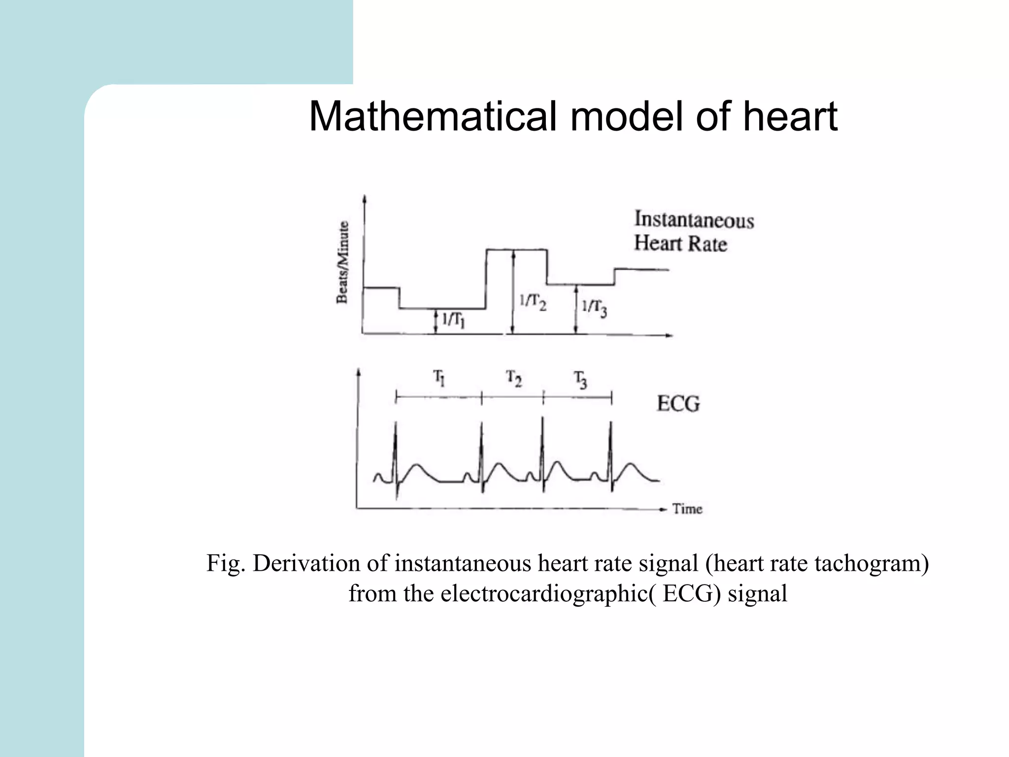
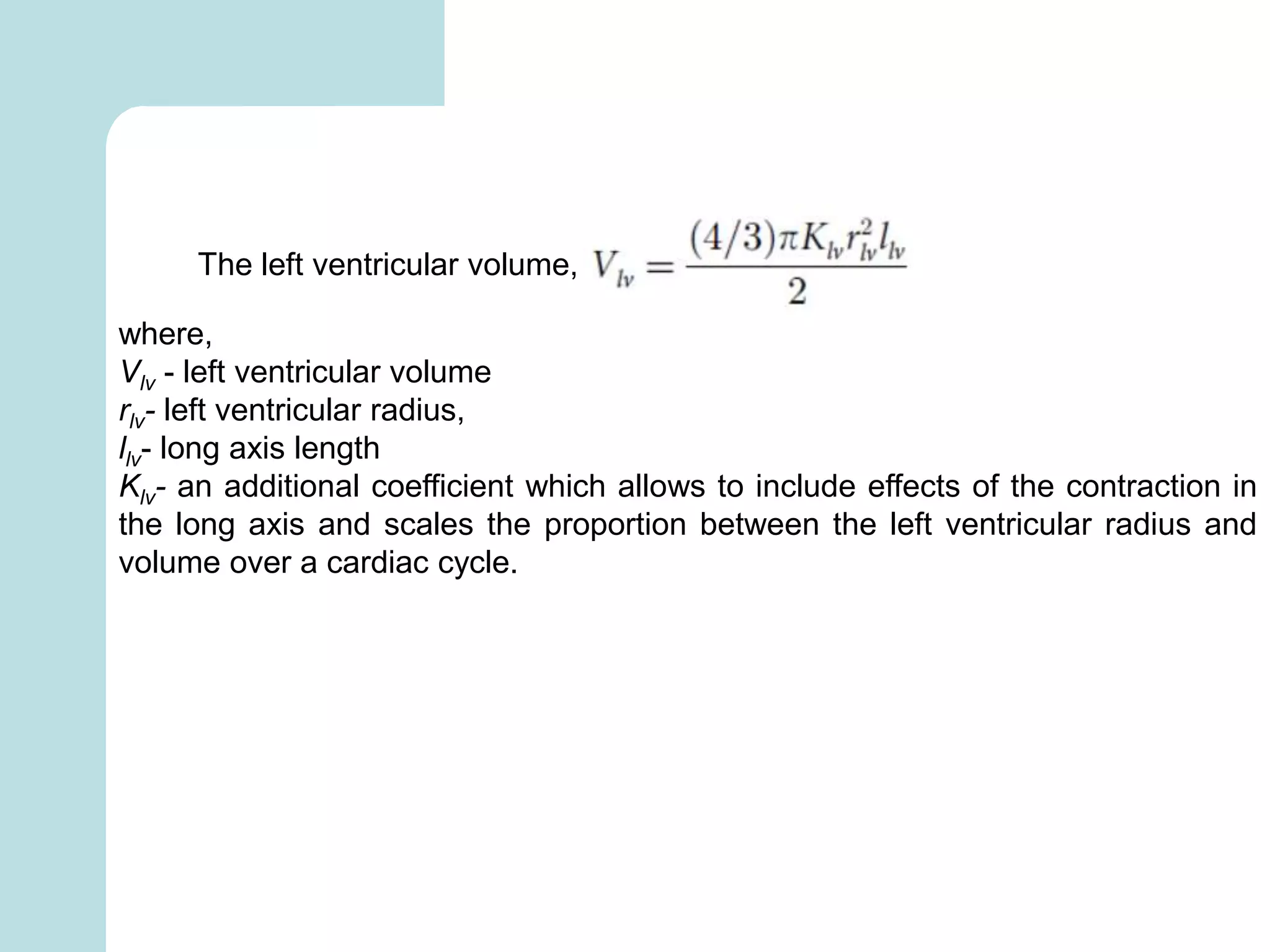
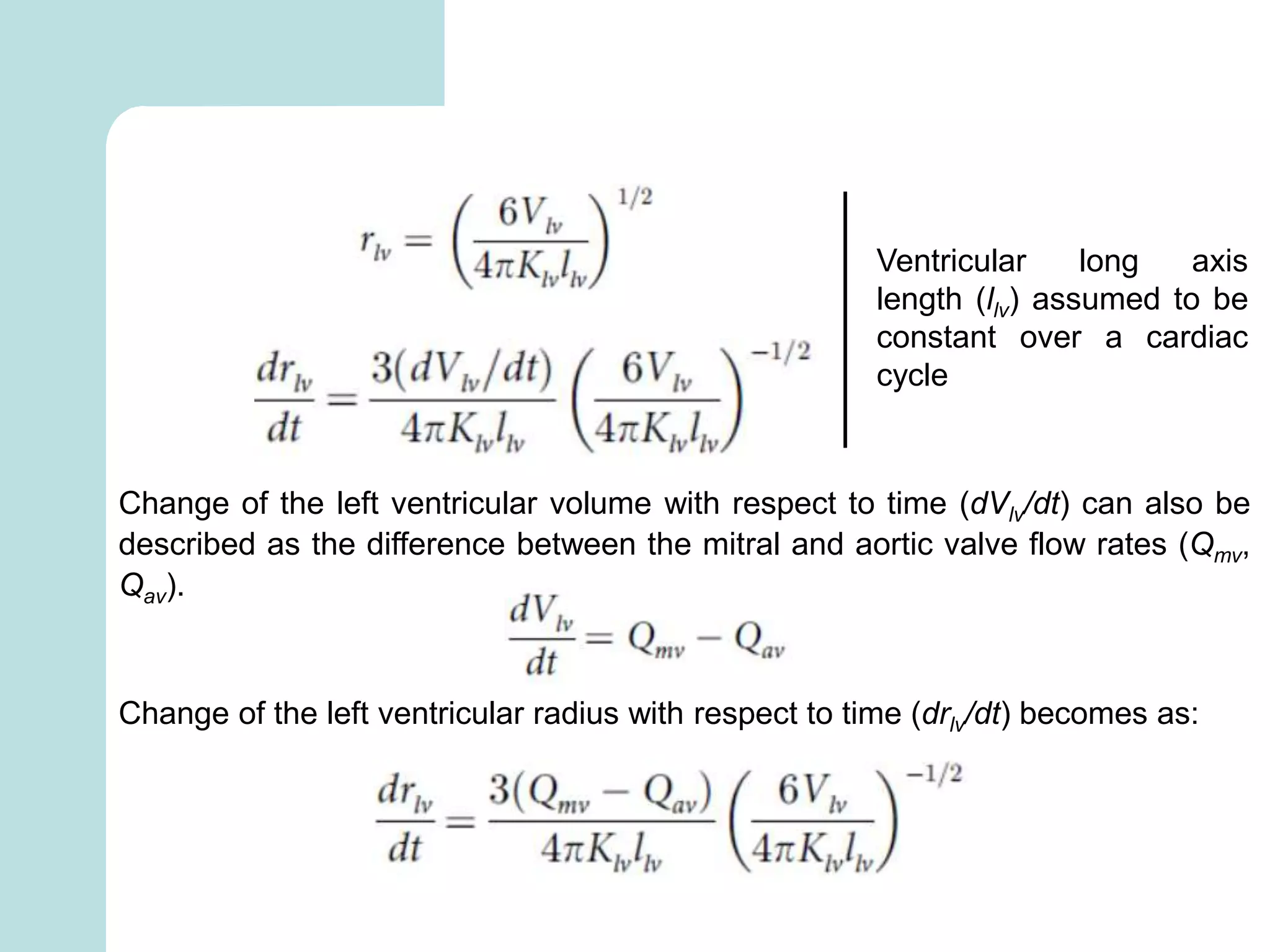
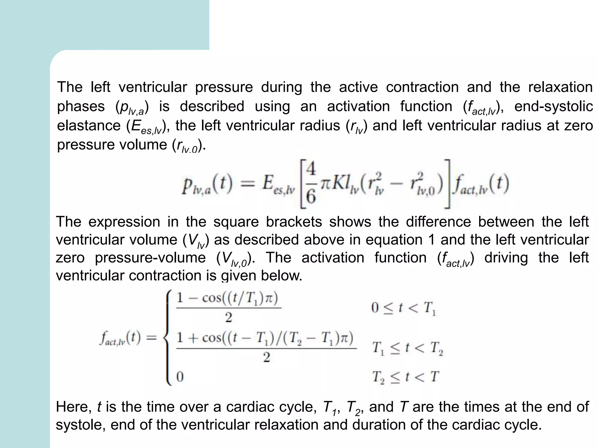
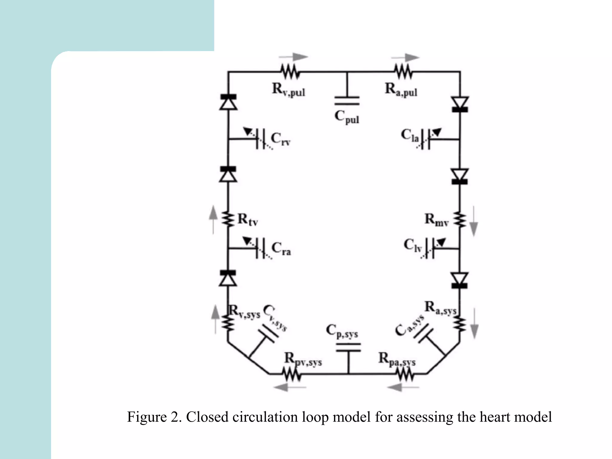
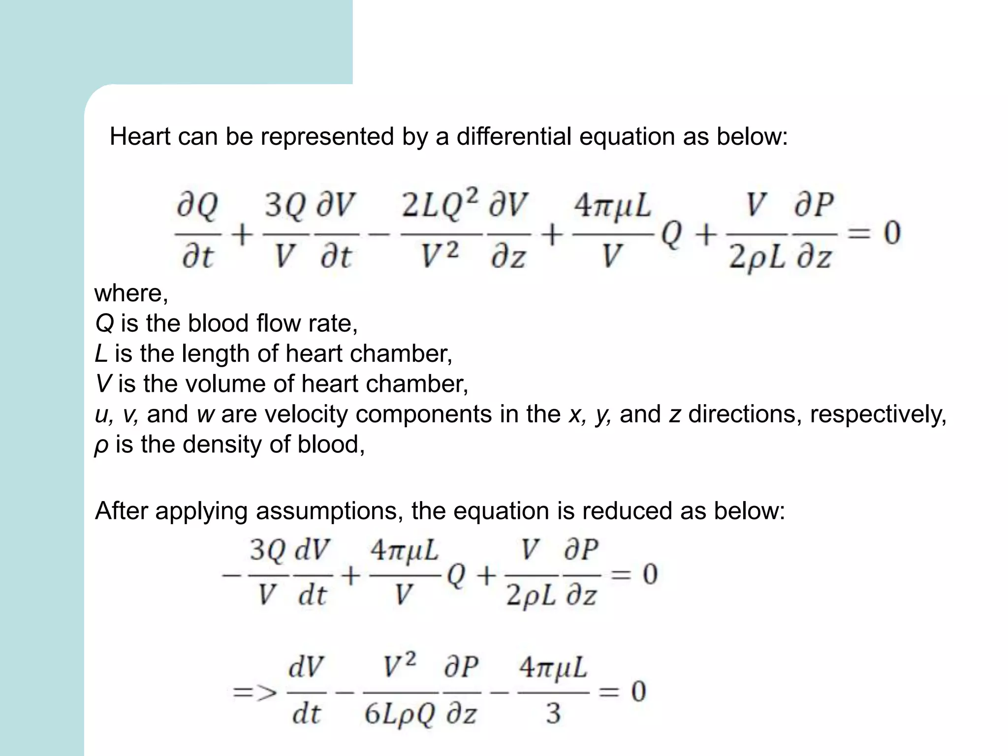
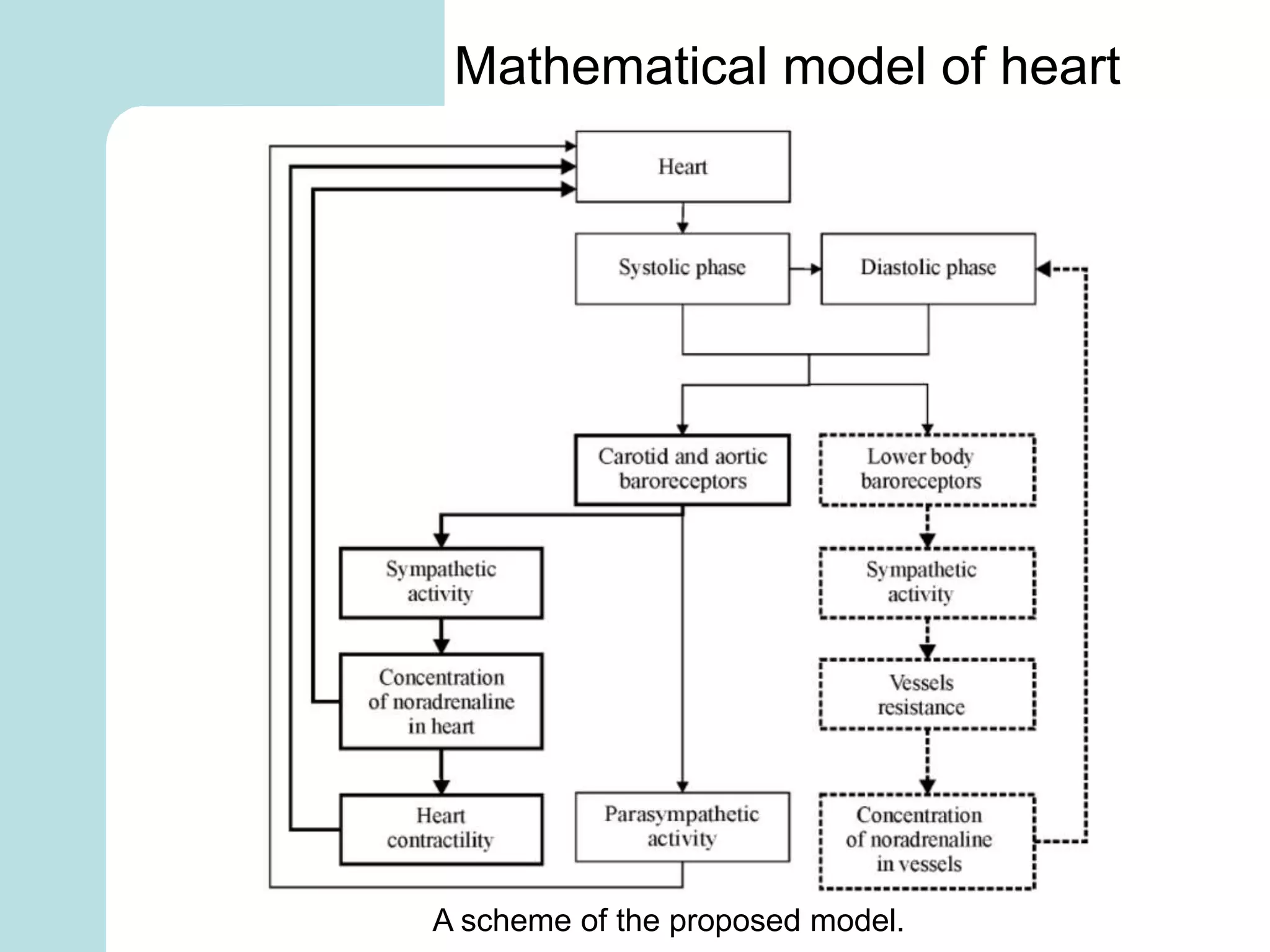
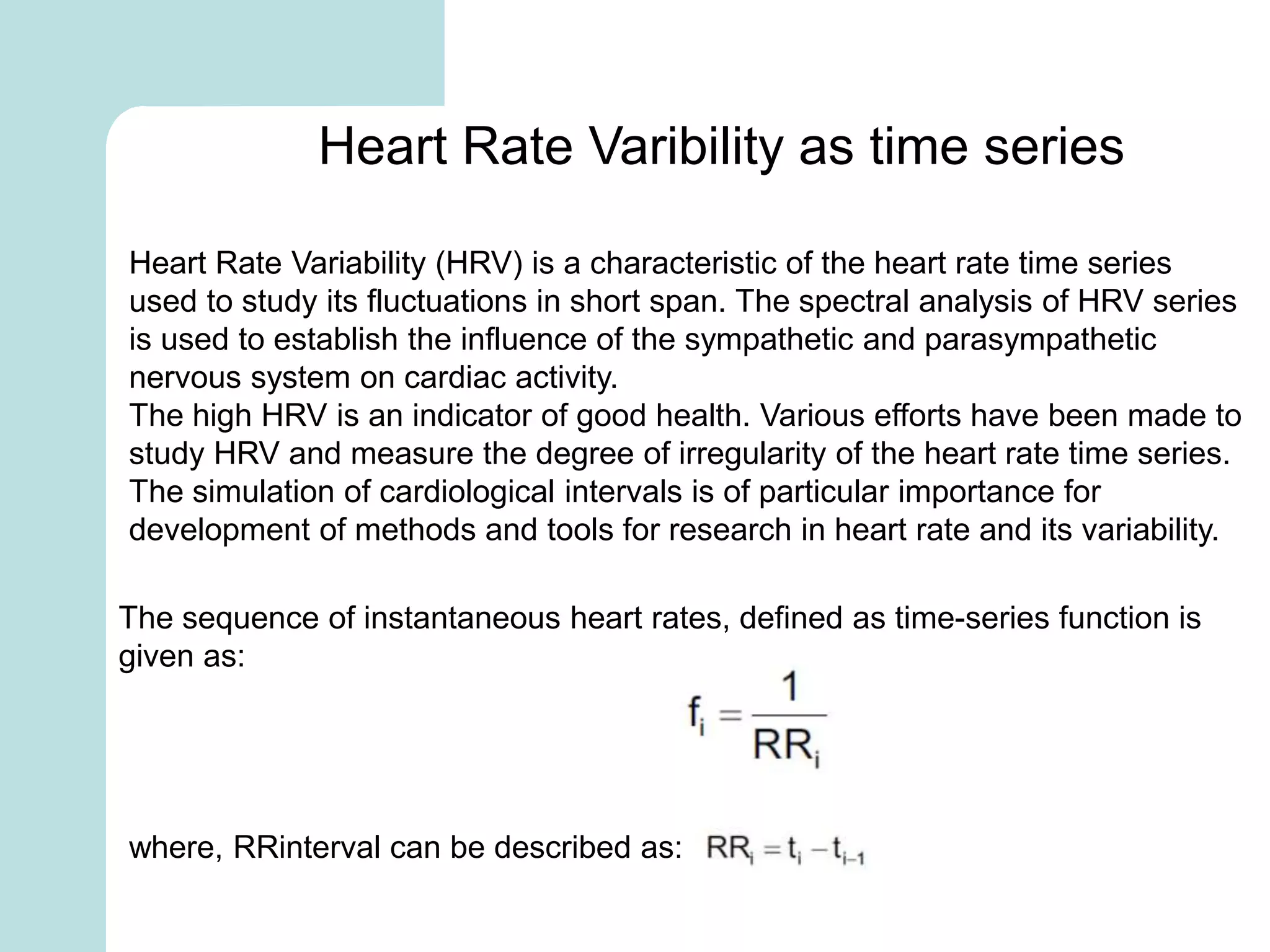
Mathematical modelling of Health care
Presented by:
Snehanshu Shekhar, (Ph. D. Scholar),
ID no-2021krec2001
Submitted to:
Dr. Ashish Sharma,
Asst. Prof., CSE Dept., IIIT Kota
Disclaimer
Copyright is not reserved by author/ presenter. Author/
presenter acknowledges all the work used for reference in
this presentation for submission of assignment. This is not
meant for any commercial purpose & only meant for
educational purpose of assignment work, following syllabus
of IIIT, Kota.
Courtesy to all authors, websites and sources of materials
used to teach.
Reader is requested to report any inadvertent typo error
contained, herein.
Table of content
Author(s) Year Work on
(mammal(s))
Heart beat rate Blood pressure Remarks/
condition
Ried Hunt and D.
W. Harrington
1897 Calf,
Opposum
Calf-156 beats/ minute
Opposum-144-218
beats/ minute
Calf-100 mm. of
mercury
Opposum-120-135
mm. of mercury
Ansesthetised
A. Rosenblueth
and F.A. Simeone
1934 Cat 150-261 beats/ minute 80-100 mm of
mercury
Ansesthetised
Deborah A. Jaye,
Yong-Fu Xiao,
and Daniel C.
Sigg
2010 Human 60-100 beats/ minute 70-130 mm of
mercury
Normal condition
Franck 1890 Cat and Dog Cat-150-261 beats/
minute
Dog-80-140 beats/
minute
Cat- 80-100 mm of
mercury
Dog- 70-145 mm
of mercury
-
Bayliss and
Starling
1892,
1902
Dog Dog-80-110 beats/
minute
Dog- 70-90 mm of
mercury
Ansesthetised
T. Hough 1892 Cat and Dog Cat-162-192 beats/
minute
Dog-80-110 beats/
minute
Cat-120-180 mm.
of mercury
Dog- 70-90 mm of
mercury
Ansesthetised
Heart-Cardiac Output
The rate at which the heart beats
can affect a value called cardiac
output (CO)
• Cardiac output is defined as the volume of blood being pumped by the heart
(ventricle) per unit time
• It is calculated by a simple formula
– CO= HR x SV
– HR= heart rate
– SV= stroke volume
Blood pressure in arteries is frequently assessed under anesthesia, whether it is
indirect (Doppler/oscillometric) or direct
• Arterial blood pressure measurement is one of the fastest and most informative
means of assessing cardiovascular function
• When it is done correctly and frequently enough, it helps provides an accurate
indication of drug effects, surgical events, and hemodynamic trends
• This is modified by almost all drugs used to induce and maintain anesthesia
Blood Pressure
ABP is typically measured as MAP (mean
arterial
pressure)
• MAP can be estimated by this formula
– Pm= Pd + 1/3 (Ps-Pd)
– Pm=mean
– Pd=diastolic
– Ps=systolic
– Systolic and diastolic can be measured
indirectly using
Doppler or oscillometric devices
• MAP is a result of CO x SVR (systemic
vascular
resistance)- which is the driving force for
blood
flow
Arterial Blood Pressure
Mathematical model of heart
Fig. Derivation of instantaneous heart rate signal (heart rate tachogram)
from the electrocardiographic( ECG) signal
The left ventricular volume,
where,
Vlv - left ventricular volume
rlv- left ventricular radius,
llv- long axis length
Klv- an additional coefficient which allows to include effects of the contraction in
the long axis and scales the proportion between the left ventricular radius and
volume over a cardiac cycle.
Ventricular long axis
length (llv) assumed to be
constant over a cardiac
cycle
Change of the left ventricular volume with respect to time (dVlv/dt) can also be
described as the difference between the mitral and aortic valve flow rates (Qmv,
Qav).
Change of the left ventricular radius with respect to time (drlv/dt) becomes as:
The left ventricular pressure during the active contraction and the relaxation
phases (plv,a) is described using an activation function (fact,lv), end-systolic
elastance (Ees,lv), the left ventricular radius (rlv) and left ventricular radius at zero
pressure volume (rlv,0).
The expression in the square brackets shows the difference between the left
ventricular volume (Vlv) as described above in equation 1 and the left ventricular
zero pressure-volume (Vlv,0). The activation function (fact,lv) driving the left
ventricular contraction is given below.
Here, t is the time over a cardiac cycle, T1, T2, and T are the times at the end of
systole, end of the ventricular relaxation and duration of the cardiac cycle.
Figure 2. Closed circulation loop model for assessing the heart model
Heart can be represented by a differential equation as below:
where,
Q is the blood flow rate,
L is the length of heart chamber,
V is the volume of heart chamber,
u, v, and w are velocity components in the x, y, and z directions, respectively,
ρ is the density of blood,
After applying assumptions, the equation is reduced as below:
A scheme of the proposed model.
Mathematical model of heart
Heart Rate Varibility as time series
Heart Rate Variability (HRV) is a characteristic of the heart rate time series
used to study its fluctuations in short span. The spectral analysis of HRV series
is used to establish the influence of the sympathetic and parasympathetic
nervous system on cardiac activity.
The high HRV is an indicator of good health. Various efforts have been made to
study HRV and measure the degree of irregularity of the heart rate time series.
The simulation of cardiological intervals is of particular importance for
development of methods and tools for research in heart rate and its variability.
The sequence of instantaneous heart rates, defined as time-series function is
given as:
where, RRinterval can be described as:
Pacemaker
Pacemaker block diagram
Electrical conductivity of heart
Mathematical modeling of health care system.ppt

Mathematical modeling of health care system.ppt

  • 1.
    Mathematical modelling ofHealth care Presented by: Snehanshu Shekhar, (Ph. D. Scholar), ID no-2021krec2001 Submitted to: Dr. Ashish Sharma, Asst. Prof., CSE Dept., IIIT Kota
  • 2.
    Disclaimer Copyright is notreserved by author/ presenter. Author/ presenter acknowledges all the work used for reference in this presentation for submission of assignment. This is not meant for any commercial purpose & only meant for educational purpose of assignment work, following syllabus of IIIT, Kota. Courtesy to all authors, websites and sources of materials used to teach. Reader is requested to report any inadvertent typo error contained, herein.
  • 3.
  • 4.
    Author(s) Year Workon (mammal(s)) Heart beat rate Blood pressure Remarks/ condition Ried Hunt and D. W. Harrington 1897 Calf, Opposum Calf-156 beats/ minute Opposum-144-218 beats/ minute Calf-100 mm. of mercury Opposum-120-135 mm. of mercury Ansesthetised A. Rosenblueth and F.A. Simeone 1934 Cat 150-261 beats/ minute 80-100 mm of mercury Ansesthetised Deborah A. Jaye, Yong-Fu Xiao, and Daniel C. Sigg 2010 Human 60-100 beats/ minute 70-130 mm of mercury Normal condition Franck 1890 Cat and Dog Cat-150-261 beats/ minute Dog-80-140 beats/ minute Cat- 80-100 mm of mercury Dog- 70-145 mm of mercury - Bayliss and Starling 1892, 1902 Dog Dog-80-110 beats/ minute Dog- 70-90 mm of mercury Ansesthetised T. Hough 1892 Cat and Dog Cat-162-192 beats/ minute Dog-80-110 beats/ minute Cat-120-180 mm. of mercury Dog- 70-90 mm of mercury Ansesthetised
  • 5.
    Heart-Cardiac Output The rateat which the heart beats can affect a value called cardiac output (CO) • Cardiac output is defined as the volume of blood being pumped by the heart (ventricle) per unit time • It is calculated by a simple formula – CO= HR x SV – HR= heart rate – SV= stroke volume
  • 6.
    Blood pressure inarteries is frequently assessed under anesthesia, whether it is indirect (Doppler/oscillometric) or direct • Arterial blood pressure measurement is one of the fastest and most informative means of assessing cardiovascular function • When it is done correctly and frequently enough, it helps provides an accurate indication of drug effects, surgical events, and hemodynamic trends • This is modified by almost all drugs used to induce and maintain anesthesia Blood Pressure
  • 7.
    ABP is typicallymeasured as MAP (mean arterial pressure) • MAP can be estimated by this formula – Pm= Pd + 1/3 (Ps-Pd) – Pm=mean – Pd=diastolic – Ps=systolic – Systolic and diastolic can be measured indirectly using Doppler or oscillometric devices • MAP is a result of CO x SVR (systemic vascular resistance)- which is the driving force for blood flow Arterial Blood Pressure
  • 8.
    Mathematical model ofheart Fig. Derivation of instantaneous heart rate signal (heart rate tachogram) from the electrocardiographic( ECG) signal
  • 9.
    The left ventricularvolume, where, Vlv - left ventricular volume rlv- left ventricular radius, llv- long axis length Klv- an additional coefficient which allows to include effects of the contraction in the long axis and scales the proportion between the left ventricular radius and volume over a cardiac cycle.
  • 10.
    Ventricular long axis length(llv) assumed to be constant over a cardiac cycle Change of the left ventricular volume with respect to time (dVlv/dt) can also be described as the difference between the mitral and aortic valve flow rates (Qmv, Qav). Change of the left ventricular radius with respect to time (drlv/dt) becomes as:
  • 11.
    The left ventricularpressure during the active contraction and the relaxation phases (plv,a) is described using an activation function (fact,lv), end-systolic elastance (Ees,lv), the left ventricular radius (rlv) and left ventricular radius at zero pressure volume (rlv,0). The expression in the square brackets shows the difference between the left ventricular volume (Vlv) as described above in equation 1 and the left ventricular zero pressure-volume (Vlv,0). The activation function (fact,lv) driving the left ventricular contraction is given below. Here, t is the time over a cardiac cycle, T1, T2, and T are the times at the end of systole, end of the ventricular relaxation and duration of the cardiac cycle.
  • 12.
    Figure 2. Closedcirculation loop model for assessing the heart model
  • 13.
    Heart can berepresented by a differential equation as below: where, Q is the blood flow rate, L is the length of heart chamber, V is the volume of heart chamber, u, v, and w are velocity components in the x, y, and z directions, respectively, ρ is the density of blood, After applying assumptions, the equation is reduced as below:
  • 14.
    A scheme ofthe proposed model. Mathematical model of heart
  • 15.
    Heart Rate Varibilityas time series Heart Rate Variability (HRV) is a characteristic of the heart rate time series used to study its fluctuations in short span. The spectral analysis of HRV series is used to establish the influence of the sympathetic and parasympathetic nervous system on cardiac activity. The high HRV is an indicator of good health. Various efforts have been made to study HRV and measure the degree of irregularity of the heart rate time series. The simulation of cardiological intervals is of particular importance for development of methods and tools for research in heart rate and its variability. The sequence of instantaneous heart rates, defined as time-series function is given as: where, RRinterval can be described as:
  • 22.
  • 23.
  • 24.