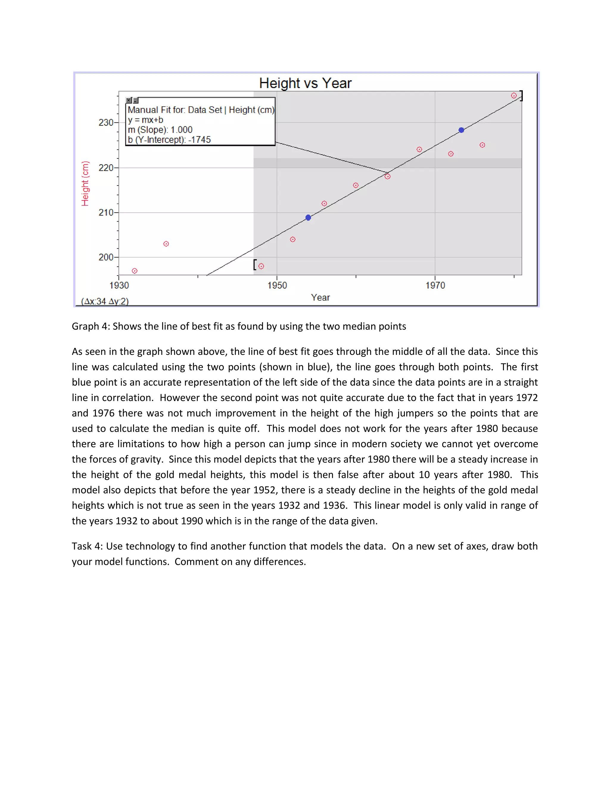
1. The document analyzes the winning heights of men's high jump gold medalists at the Olympic Games from 1896 to 2008. Various mathematical models are tested to fit the data, including linear, logarithmic, cubic, and Gaussian functions. 2. The initial linear model is found to fit the data reasonably from 1932 to around 1990 but fails outside this range. A modified logarithmic model provides a better fit overall but still has limitations. 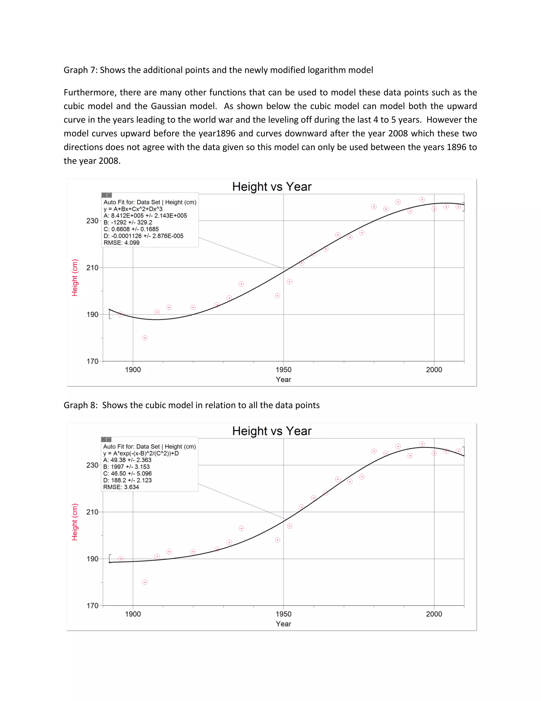3. Cubic and Gaussian models also show good fits for parts of the data trend but cannot fully represent fluctuations throughout the entire data set from 1896 to 2008. Further refinement of models is needed to accurately capture the entire trend over time.

1. Non Sereeyothin
Math Period 3
May 19, 2011
Gold Medal Heights
Objective: to consider the winning height for the men’s high jump in the Olympic Games.
The table below gives the height (in centimeter) achieved by the gold medalists at various Olympic
Games.
Year 1932 1936 1948 1952 1956 1960 1964 1968 1972 1976 1980
Height 197 203 198 204 212 216 218 224 223 225 236
(cm)
Note: The Olympic Games were not held in 1940 and 1944.
Task 1: Using technology, plot the data points on a graph. Define all variables used and state any
parameters clearly. Discuss any possible constraints of the task.
Graph 1: This graph shows the correlation between the year and the height of the gold medal winners in
the Olympic. The x-axis on this graph presents the years that the data was collect while the y-axis
presents the height of the gold winner of that current year. This graph was graphed using logger pro.
Constraints: During the years 1940 and 1944, the Olympic was cancelled due to the world war. Due to
this, the data point does not continue according to its intervals of 4 years. It can be assumed that the

2. high jumpers lost their practicing times during the world war, limiting their ability to improve on their
skill, making the highest jumper in the year 1948 when the Olympic resumed lower than that of the
previous year. Because of this the first two data points can be eliminated from the calculation of the
equation due to the fact that the trend seems to start over at the year 1948.
Task 2: What type of function models the behavior of the graph? Explain why you chose this function.
Analytically create an equation to model the data in the above table.
The function that models the behavior of the graph the best is a linear function since the graph trends to
correlate in a straight line as shown by the line of best fit.
Calculation: To calculate the line of best fit, the data points were split in half by the green line and a
point was chosen to be the median of both sides as shown below.
Graph 2: Shows the midline splitting the data into two sections and the point that are chosen on both
sides to represent the median.
An equation was then found that went through both the points. This equation was then used as the line
of best fit for the data. The equation y=mx+b was used to calculate the line of best fit since the trend of
that data seemed to be linear.

3. Graph 3: Shows the two new points in comparison to the rest of the data
By using the coordinates of the two points, the equation of the line of best was found as shown below.
-1745.12
Task 3: On a new set of axes, draw your model function and the original graph. Comment on any
differences. Discuss the limitations of your model. Refine your model is necessary.

4. Graph 4: Shows the line of best fit as found by using the two median points
As seen in the graph shown above, the line of best fit goes through the middle of all the data. Since this
line was calculated using the two points (shown in blue), the line goes through both points. The first
blue point is an accurate representation of the left side of the data since the data points are in a straight
line in correlation. However the second point was not quite accurate due to the fact that in years 1972
and 1976 there was not much improvement in the height of the high jumpers so the points that are
used to calculate the median is quite off. This model does not work for the years after 1980 because
there are limitations to how high a person can jump since in modern society we cannot yet overcome
the forces of gravity. Since this model depicts that the years after 1980 there will be a steady increase in
the height of the gold medal heights, this model is then false after about 10 years after 1980. This
model also depicts that before the year 1952, there is a steady decline in the heights of the gold medal
heights which is not true as seen in the years 1932 and 1936. This linear model is only valid in range of
the years 1932 to about 1990 which is in the range of the data given.
Task 4: Use technology to find another function that models the data. On a new set of axes, draw both
your model functions. Comment on any differences.

5. Graph 5: Shows both models (linear and logarithm) in relative to each other
The equation used to model the line on bottom is the natural logarithm model while the equation used
to model the line above is the linear model. When comparing the two models, the difference between
the two is that the y-intercept is lower for the natural logarithm model than the linear model and the
slope appears to be quite parallel.
Task 5: Had the games been held in 1940 and 1944, estimate what the winning heights would have been
and justify your answers.
Using the natural logarithm model as the function, the years 1940 and 1944 were plugged into the
equation and the heights of both years are calculated as shown below.
( )
( )
( )
Due to the elimination of the first two points, the estimation of the years 1940 and 1944 will be lower
than expected because the slope of the graph will be much higher.
Task 6: Use your model to predict the winning height in 1984 and in 2016. Comment on your answers.

6. ( )
( )
( )
The height estimated by this model in the year 1984 seems credible since the increase in height does not
seem to be out of reach of the human capability. However, in the year 2016, the height that was
reached was 270cm which seems to be higher than a human can possibly jump. This is because the
natural logarithm model depicts a straight line following the year 1980 and because a steady increase in
the heights of the Olympic high jumpers does not seem possible for a human being, the further away
from the year 1980 the lower the credibility of the answer.
The following table gives the winning heights for all the other Olympic Games since 1896.
Year 1896 1904 1908 1912 1920 1928 1932 1936 1948 1952 1956
Height 190 180 191 193 193 194 197 203 198 204 212
(cm)
Year 1960 1964 1968 1972 1976 1980 1984 1988 1992 1996 2000 2004 2008
Height 216 218 224 223 225 236 235 238 234 239 235 236 236
(cm)
Task 7: How well does your model fit the additional data? Discuss the overall trend from 1896 to 2008,
with specific references to significant fluctuations. What modifications, if any, need to be made to your
made to fit the data?

7. Graph 6: Shows the logarithm model with additional points of data
The model that was used to find the line of best fit in the last task does not fit the additional data. This
is because during the year 1896 and 2008 there has been fluctuations in the height of the gold winners.
The data starts out as a straight line with an outlier in the year 1904 then curves upwards in the years
leading up to the world war (1928, 1932, 1936). During the world war the heights was assumed to have
dropped due to the lost in practice times so the trend starts again in 1948 with a straight linear
correlation all the way through to the year 1988. After that the data seems to level off into a horizontal
correlation.
The modification that needs to be made to the model is that all data points must be included to have a
better sense of the median and range of the data to be more accurate as shown below.

8. Graph 7: Shows the additional points and the newly modified logarithm model
Furthermore, there are many other functions that can be used to model these data points such as the
cubic model and the Gaussian model. As shown below the cubic model can model both the upward
curve in the years leading to the world war and the leveling off during the last 4 to 5 years. However the
model curves upward before the year1896 and curves downward after the year 2008 which these two
directions does not agree with the data given so this model can only be used between the years 1896 to
the year 2008.
Graph 8: Shows the cubic model in relation to all the data points

9. Graph 9: Shows the Gaussian model in relationship to all the data points
The Gaussian model can also be used to model this part of the data but it is different from the cubic
model since the Gaussian model starts off with a level and horizontal line then curves up similarly to the
cubic model. In addition to that the Gaussian model also models the leveling off as the years approach
2008 but has the same limitation as the cubic model as the graph slopes back downwards after the year
2008. The Gaussian model is a better representation of the data since at the beginning of the data rage
the slow does not curve downward before going back upwards like the cubic model. However, the
disadvantage that the Gaussian model and the cubic model have is that they both do not show the
fluctuation of the heights of the gold medalists during the year 1821 to the year 1896 (1821 being the
year that the Olympics started).